Comparison of Multi-Physical Coupling Analysis of a Balanced Armature Receiver between the Lumped Parameter Method and the Finite Element/Boundary Element Method


Abstract
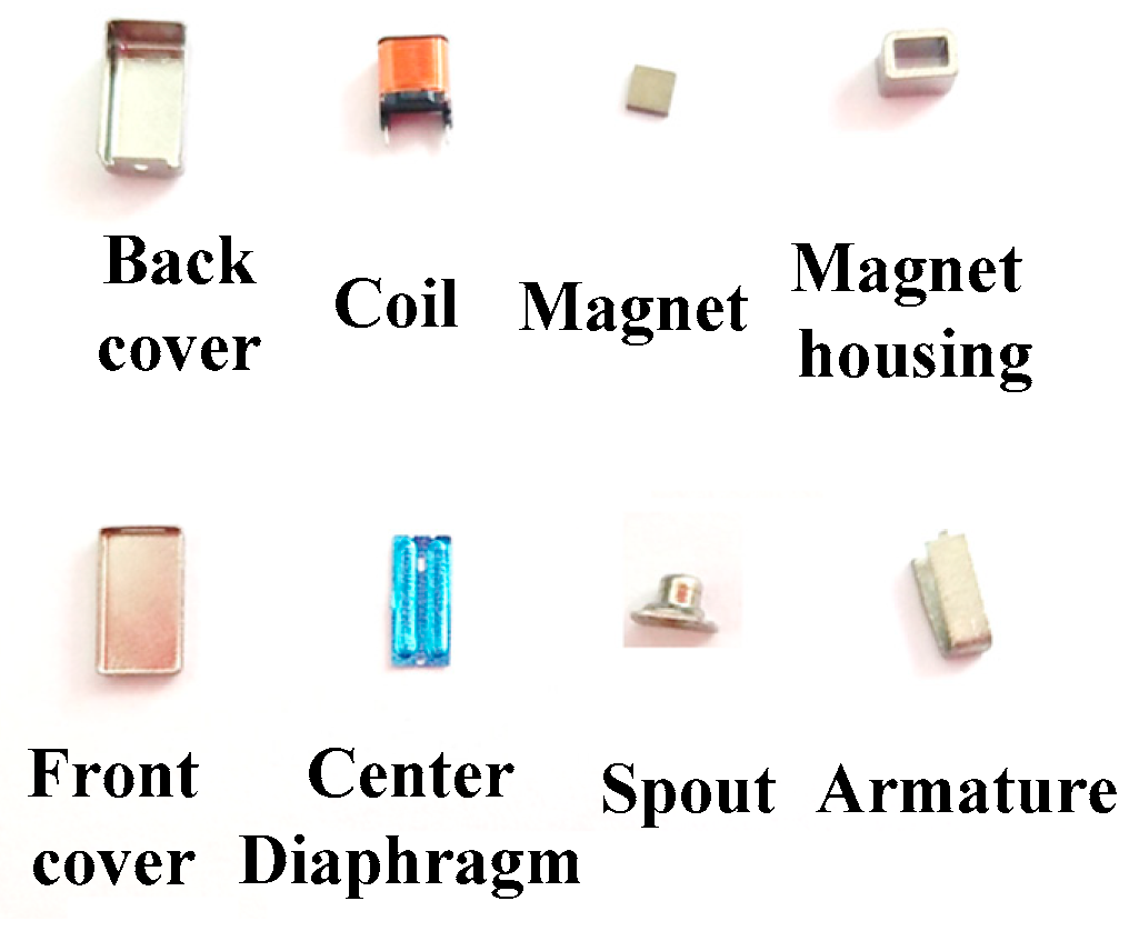
:1. Introduction
2. Analysis by LPM
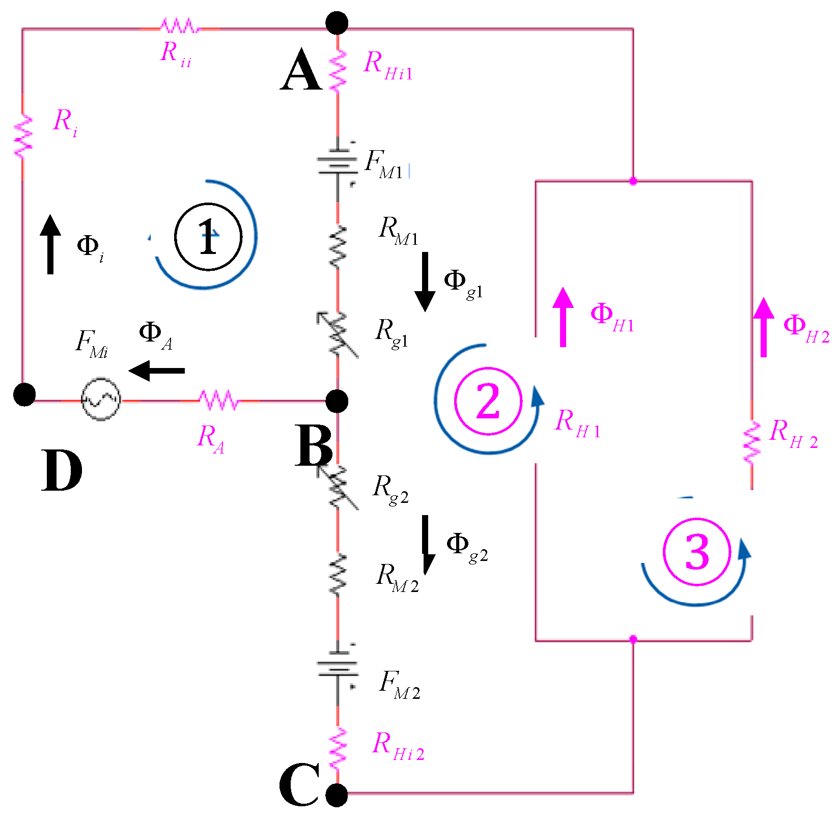
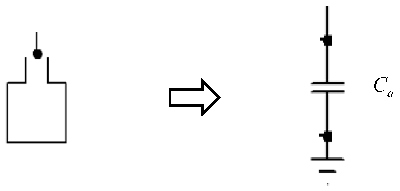
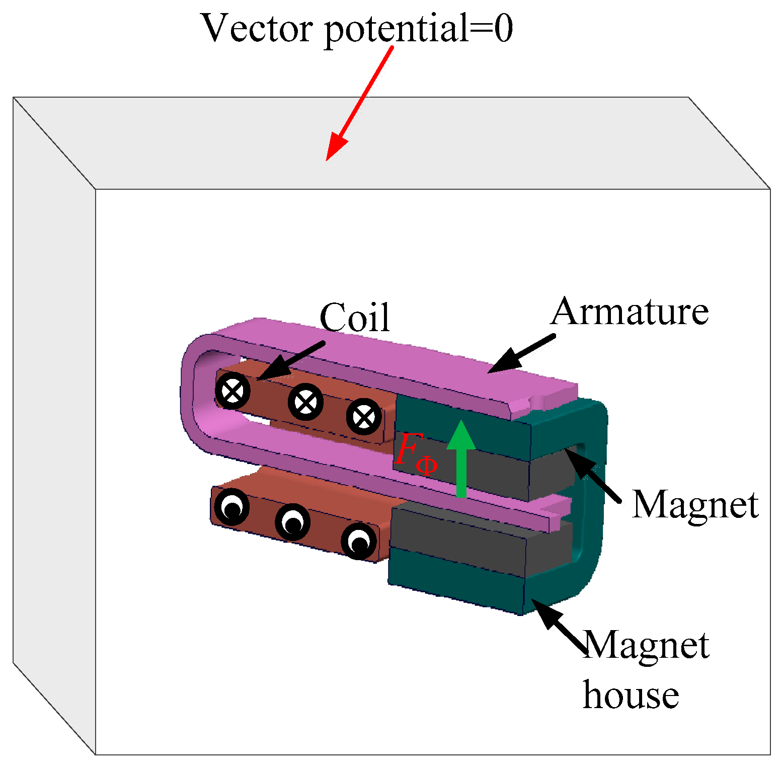
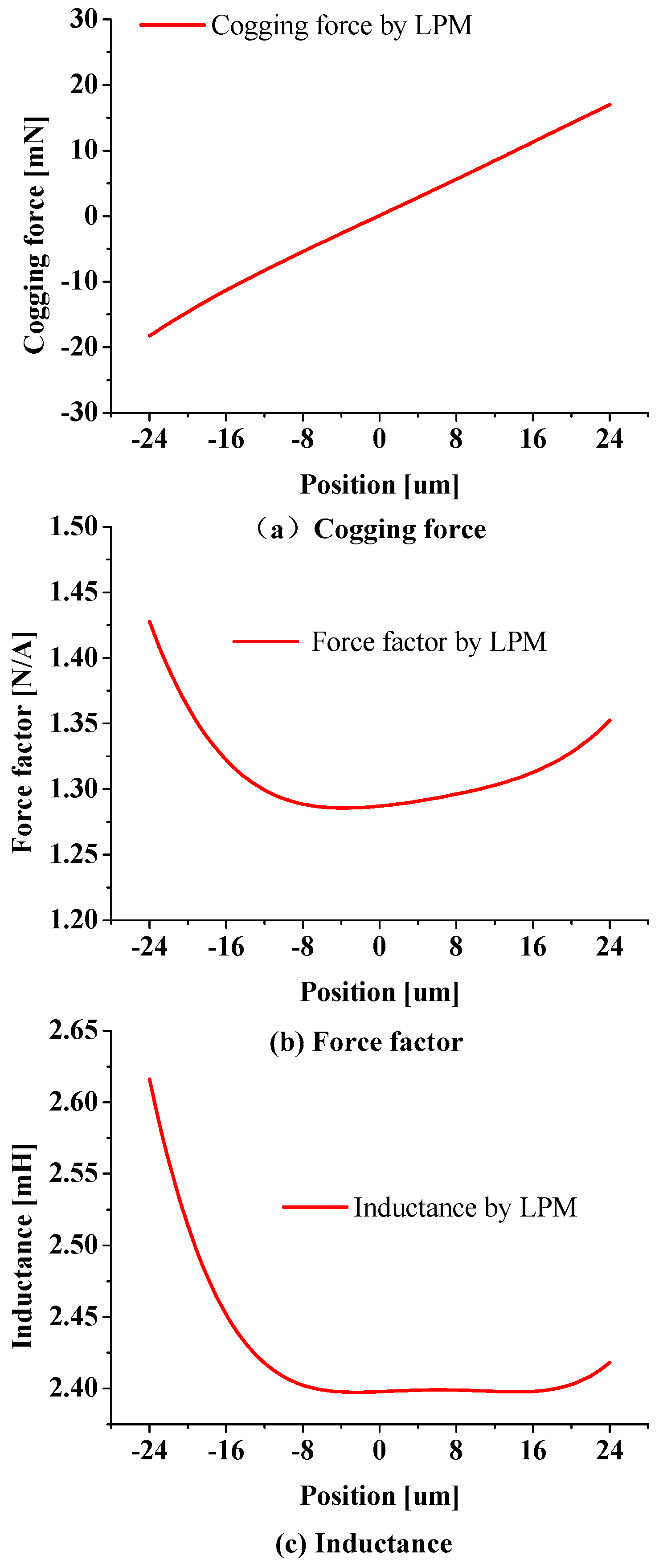
2.1. Electromagnetic Analysis
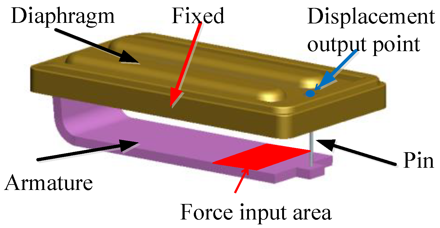
2.2. Mechanical Analysis
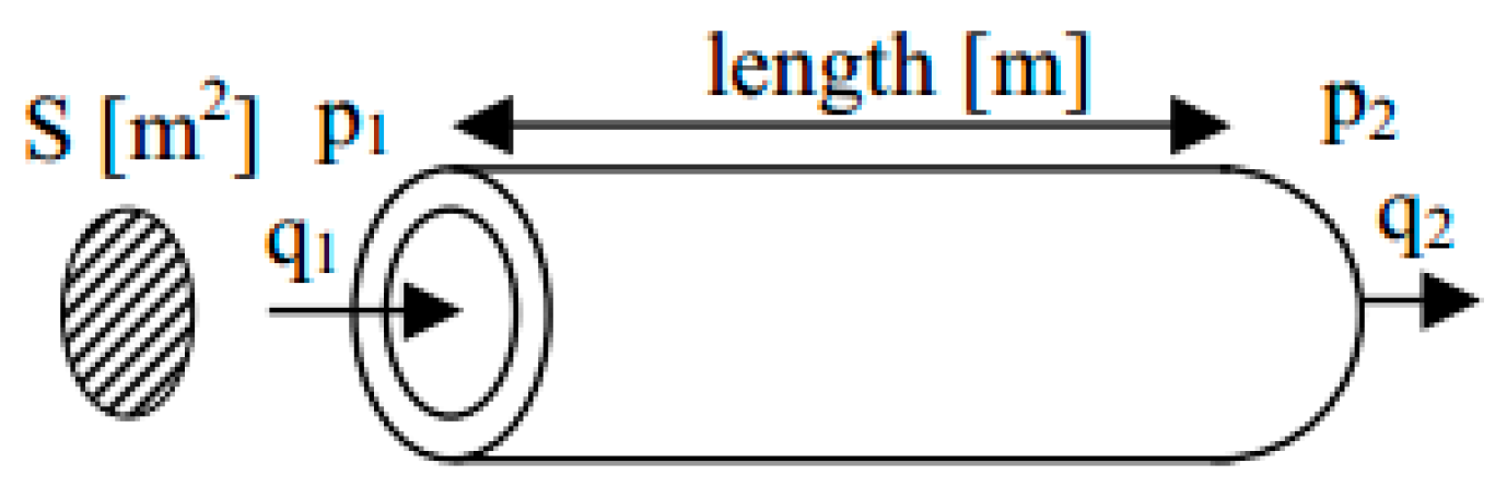
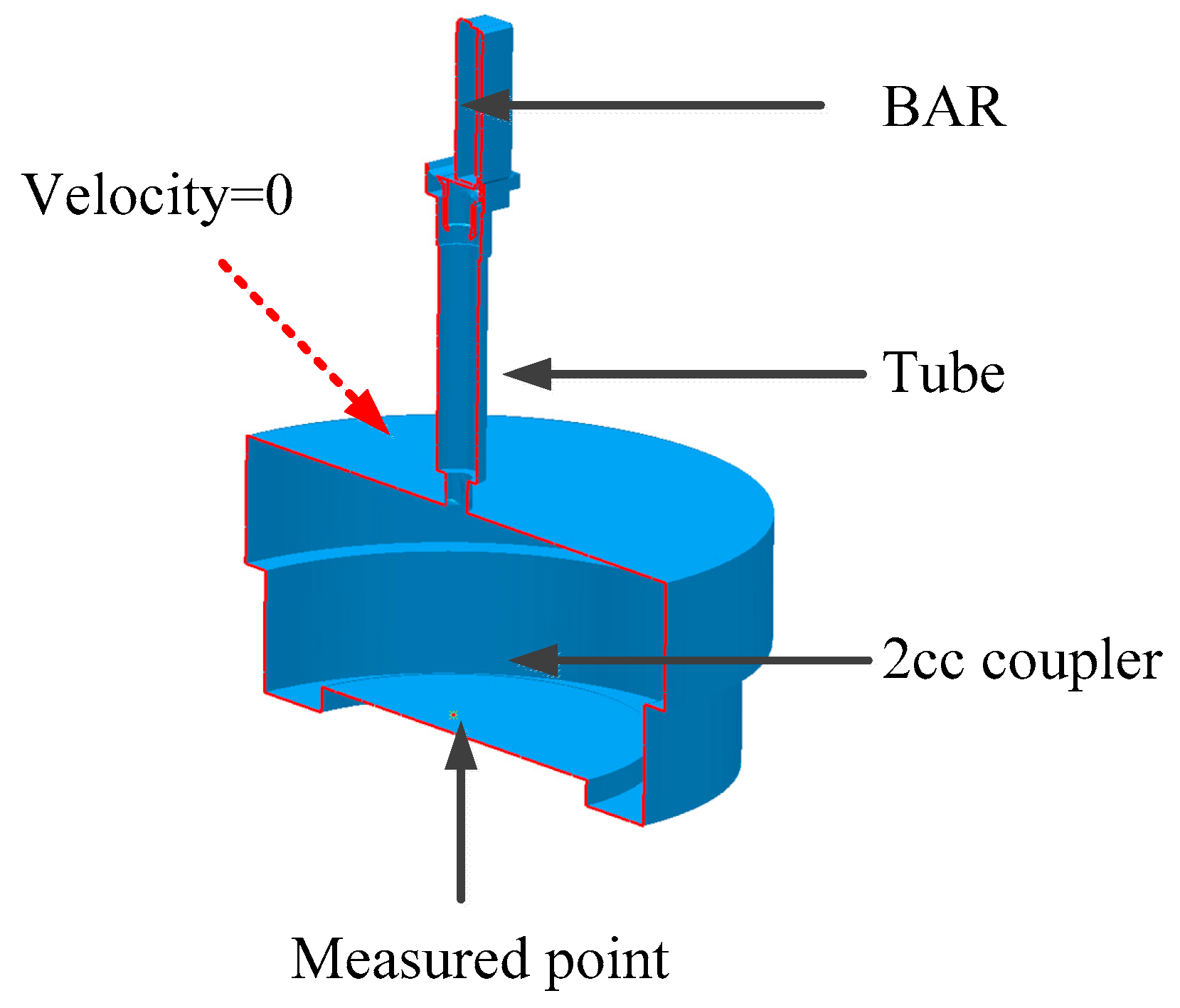
2.3. Acoustic Analysis
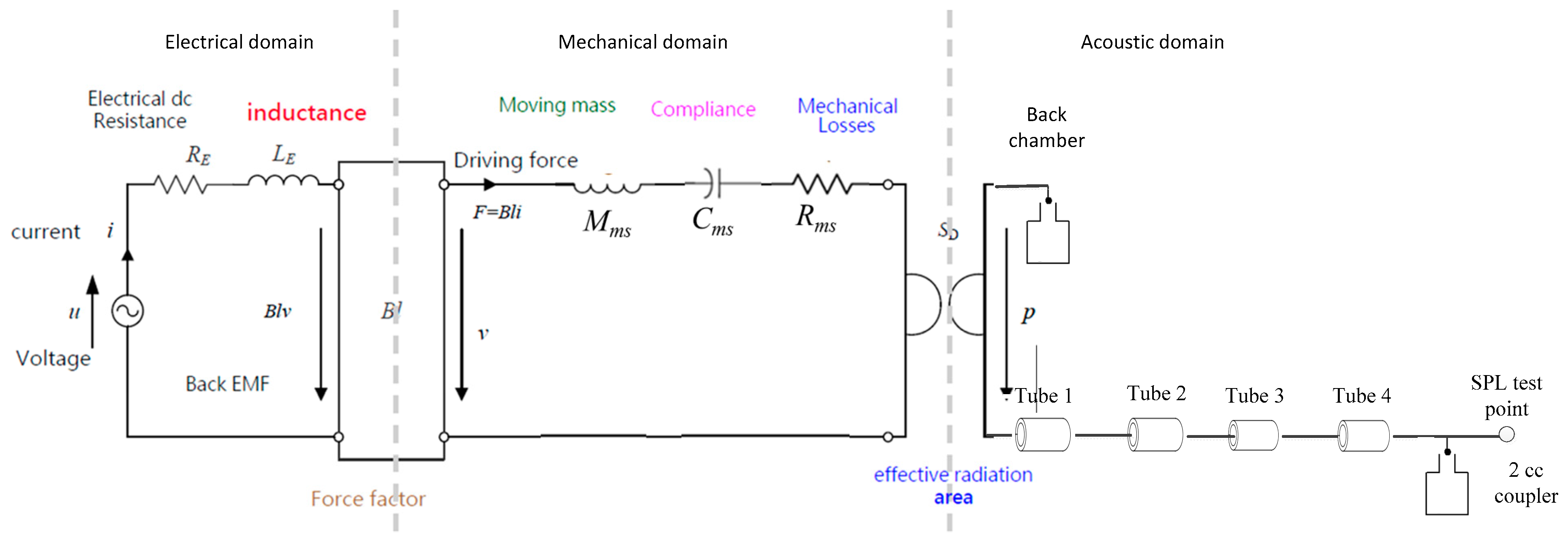
2.4. Electromagnetic-Mechanical–Acoustic Coupling Factors
3. Analysis by FEM and BEM
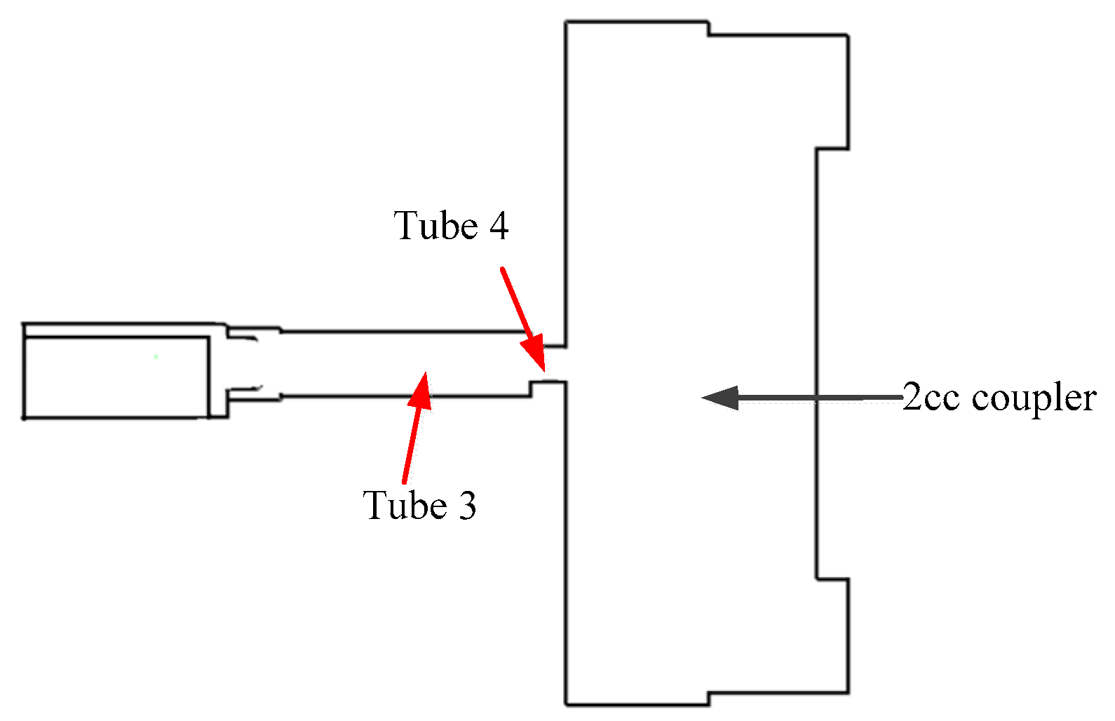
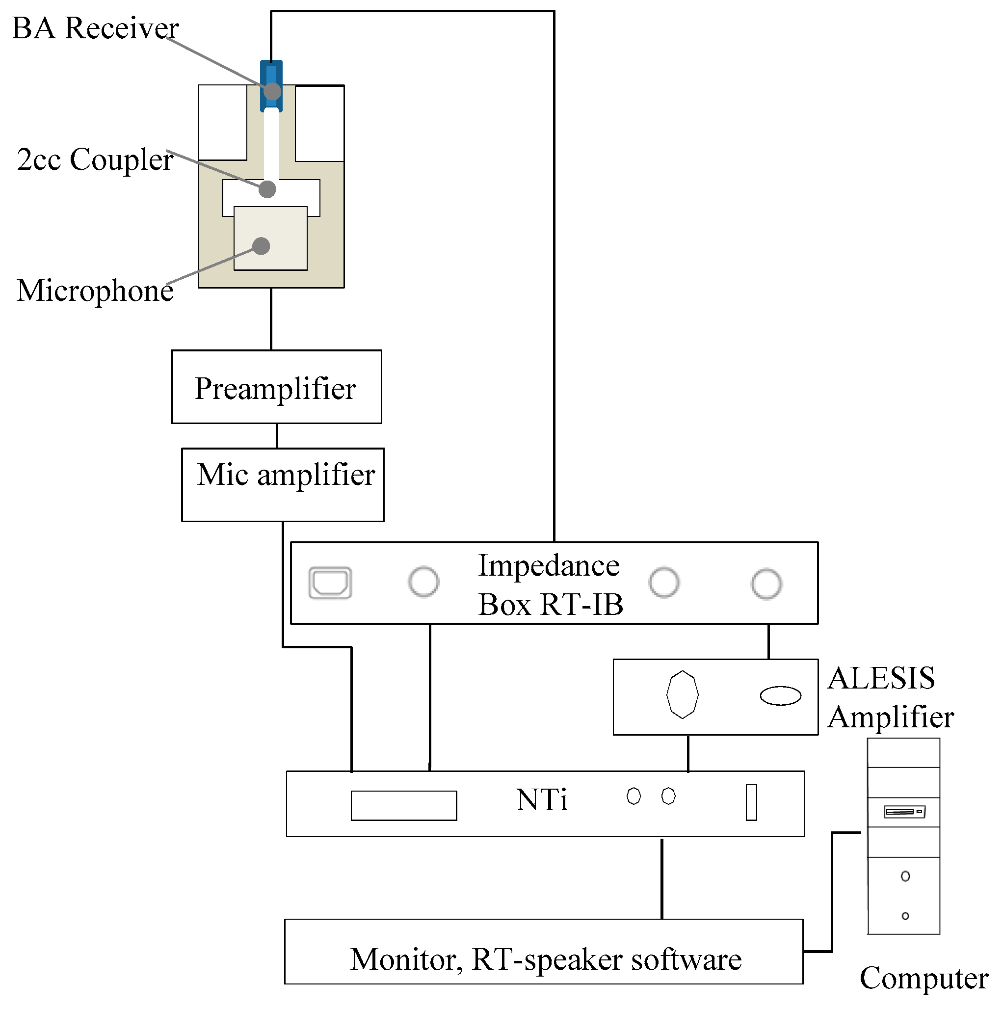
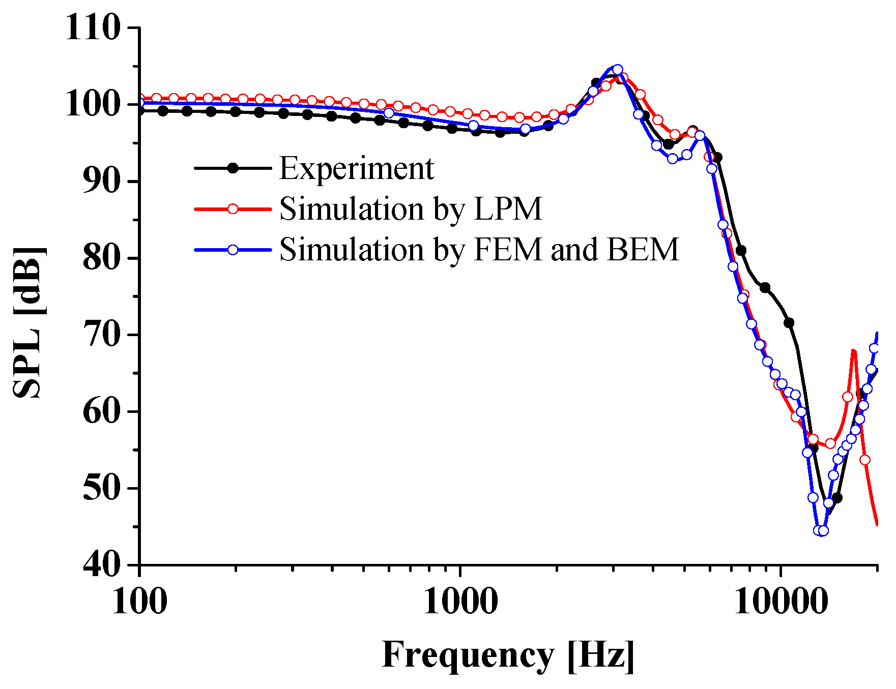
4. Experiment
5. Conclusions
Author Contributions
Funding
Conflicts of Interest
Abbreviations
| SPL | Sound pressure level |
| MEMS | Micro-Electro-Mechanical System |
| LPM | Lumped parameter method |
| FEM | Finite element method |
| BEM | Boundary element method |
| BAR | Balanced armature receiver |
| EMF | Electromotive force |
| 2-cc | 2 cubic centimeter |
References
- Zhao, C.; Knisely, K.E.; Grosh, K. Design and fabrication of a piezoelectric MEMS xylophone transducer with a flexible electrical connection. Sens. Actuators A Phys. 2018, 275, 29–36. [Google Scholar] [CrossRef]
- Zhao, C.; Knisely, K.E.; Grosh, K. Modeling, fabrication, and testing of a MEMS multichannel aln transducer for a completely implantable cochelar implant. In Proceedings of the 2017 19th International Conference on Solid-State Sensors, Actuators and Microsystems (TRANSDUCERS), Kaohsiung, Taiwan, 18–22 June 2017; pp. 16–19. [Google Scholar]
- Hwang, S.M.; Lee, H.J.; Kim, J.H.; Hwang, G.Y.; Lee, W.Y.; Kang, B.S. New development of integrated microspeaker and dynamic receiver used for cellular phones. IEEE Trans. Magn. 2003, 39, 3259–3261. [Google Scholar] [CrossRef]
- Jiang, Y.W.; Kwon, J.H.; Kim, H.K.; Hwang, S.M. Analysis and Optimization of Micro Speaker-Box Using a Passive Radiator in Portable Device. Arch. Acoust. 2017, 42, 753–760. [Google Scholar] [CrossRef] [Green Version]
- Olson, H.F. Dynamical Analogies; Van Nostrand: New York, NY, USA, 1943; pp. 126–148. [Google Scholar]
- Bauer, B.B. Magnetic Translating Device. U.S. Patent 2,454,425, 23 November 1948. [Google Scholar]
- Bauer, B. A miniature microphone for transistorized amplifiers. Trans. IRE Prof. Group Audio 1953, 1, 5–7. [Google Scholar] [CrossRef]
- Bernhard, H.; Stieger, C.; Perriard, Y. New implantable hearing device based on a micro-actuator that is directly coupled to the inner ear fluid. In Proceedings of the 2006 International Conference of the IEEE Engineering in Medicine and Biology Society, New York, NY, USA, 30 August–3 September 2006; pp. 3162–3165. [Google Scholar]
- Håkansson, B.E.V. The balanced electromagnetic separation transducer: A new bone conduction transducer. J. Acoust. Soc. Am. 2003, 113, 818–825. [Google Scholar] [CrossRef] [PubMed]
- Jayanth, V.; Nepomuceno, H.G. Balanced Armature Bone Conduction Shaker. U.S. Patent 7,869,610, 11 January 2011. [Google Scholar]
- Blanchard, M.A.; Geswein, B.C.; Hruza, E.A.; Geschiere, O. Balanced Armature with Acoustic Low Pass Filter. U.S. Patent 8,135,163, 13 March 2012. [Google Scholar]
- Jensen, J.; Agerkvist, F.T.; Harte, J.M. Nonlinear time-domain modeling of balanced-armature receivers. J. Audio Eng. Soc. 2011, 59, 91–101. [Google Scholar]
- Ziolkowski, M.; Kwiatkowski, W.; Gratkowski, S.; Ziolkowski, M. Static analysis of a balanced armature receiver. COMPEL Int. J. Comput. Math. Electr. Electron. Eng. 2018, 37, 1392–1404. [Google Scholar] [CrossRef]
- Sun, W.; Hu, W. Lumped element multimode modeling of balanced-armature receiver using modal analysis. J. Vib. Acoust. 2016, 138, 061017. [Google Scholar] [CrossRef]
- Sun, W.; Hu, W. Lumped Element Multimode Modeling for a Simplified Balanced-Armature Receiver. In Proceedings of the 23rd International Congress on Sound and Vibration, Athens, Greece, 10–14 July 2016. [Google Scholar]
- Kim, N.; Allen, J.B. Two-port network analysis and modeling of a balanced armature receiver. Hear. Res. 2013, 301, 156–167. [Google Scholar] [CrossRef] [PubMed]
- Tsai, Y.-T.; Huang, J.H. A study of nonlinear harmonic distortion in a balanced armature actuator with asymmetrical magnetic flux. Sens. Actuators A Phys. 2013, 203, 324–334. [Google Scholar] [CrossRef]
- Bai, M.R.; You, B.-C.; Lo, Y.-Y. ‘Electroacoustic analysis, design, and implementation of a small balanced armature speaker. J. Acoust. Soc. Am. 2014, 136, 2554–2560. [Google Scholar] [CrossRef] [PubMed]
- Xu, D.P.; Lu, H.W.; Jiang, Y.W.; Kim, H.K.; Kwon, J.H.; Hwang, S.M. Analysis of Sound Pressure Level of a Balanced Armature Receiver Considering Coupling Effects. IEEE Access 2017, 5, 8930–8939. [Google Scholar] [CrossRef]
- Jiang, Y.W.; Xu, D.P.; Hwang, S.M. Electromagnetic-Mechanical Analysis of a Balanced Armature Receiver by Considering the Nonlinear Parameters as a Function of Displacement and Current. IEEE Trans. Magn. 2018, 99, 1–4. [Google Scholar]
- Furlani, E.P. Permanent Magnet and Electromechanical Devices: Materials, Analysis, and Applications; Academic Press: Cambridge, MA, USA, 2001; pp. 335–345. [Google Scholar]
- Campbell, P. Permanent Magnet Materials and Their Application; Cambridge University Press: Cambridge, UK, 1996. [Google Scholar]
- Asghari, B.; Dinavahi, V. Novel transmission line modeling method for nonlinear permeance network based simulation of induction machines. IEEE Trans. Magn. 2011, 47, 2100–2108. [Google Scholar] [CrossRef]


| Domain | Proposed Method | Previous Method |
|---|---|---|
| Electromagnetic | LPM | FEM |
| Mechanical | LPM | FEM |
| Acoustic | LPM | BEM |
| Domain | Package | Elements Order | Number of Nodes |
|---|---|---|---|
| Electromagnetic | ANSYS | 3 | 146817 |
| Mechanical | ANSYS | 3 | 525006 |
| Acoustic | Virtual lab | 2 | 1329 |
| Domain | Value | Unit |
|---|---|---|
| Total dimension | 5 × 3 × 2.6 | mm |
| Coil resistance | 23 | Ohm |
| Input voltage | 0.115 | V |
© 2019 by the authors. Licensee MDPI, Basel, Switzerland. This article is an open access article distributed under the terms and conditions of the Creative Commons Attribution (CC BY) license (http://creativecommons.org/licenses/by/4.0/).
Share and Cite
Jiang, Y.-W.; Xu, D.-P.; Jiang, Z.-X.; Kim, J.-H.; Hwang, S.-M. Comparison of Multi-Physical Coupling Analysis of a Balanced Armature Receiver between the Lumped Parameter Method and the Finite Element/Boundary Element Method. Appl. Sci. 2019, 9, 839. https://doi.org/10.3390/app9050839
Jiang Y-W, Xu D-P, Jiang Z-X, Kim J-H, Hwang S-M. Comparison of Multi-Physical Coupling Analysis of a Balanced Armature Receiver between the Lumped Parameter Method and the Finite Element/Boundary Element Method. Applied Sciences. 2019; 9(5):839. https://doi.org/10.3390/app9050839
Chicago/Turabian StyleJiang, Yuan-Wu, Dan-Ping Xu, Zhi-Xiong Jiang, Jun-Hyung Kim, and Sang-Moon Hwang. 2019. "Comparison of Multi-Physical Coupling Analysis of a Balanced Armature Receiver between the Lumped Parameter Method and the Finite Element/Boundary Element Method" Applied Sciences 9, no. 5: 839. https://doi.org/10.3390/app9050839