Article

Feature Adaptive and Cyclic Dynamic Learning Based on Infinite Term Memory Extreme Learning Machine

by
Ahmed Salih AL-Khaleefa
1,*,
Mohd Riduan Ahmad
1,
Azmi Awang Md Isa
1,
Mona Riza Mohd Esa
2,
Ahmed AL-Saffar
3 and
Mustafa Hamid Hassan
4
1
Broadband and Networking (BBNET) Research Group, Centre for Telecommunication and Research Innovation (CeTRI), Fakulti Kejuruteraan Elektronik dan Kejuruteraan Komputer (FKEKK), Universiti Teknikal Malaysia Melaka (UTeM), Hang Tuah Jaya, 76100 Durian Tunggal, Melaka, Malaysia
2
Institute of High Voltage and High Current (IVAT), School of Electrical Engineering, Faculty of Engineering, Universiti Teknologi Malaysia (UTM), 81310 Skudai, Johor Bharu, Malaysia
3
Faculty of Computer System and Software Engineering, University Malaysia Pahang (UMP), 26300 Gambang, Pahang, Malaysia
4
Faculty of Computer Science and Information Technology, Universiti Tun Hussein Onn Malaysia, 86400 Batu Pahat, Johor, Malaysia
*
Author to whom correspondence should be addressed.
Appl. Sci. 2019, 9(5), 895; https://doi.org/10.3390/app9050895
Submission received: 28 January 2019 / Revised: 26 February 2019 / Accepted: 27 February 2019 / Published: 2 March 2019

Abstract

:
Online learning is the capability of a machine-learning model to update knowledge without retraining the system when new, labeled data becomes available. Good online learning performance can be achieved through the ability to handle changing features and preserve existing knowledge for future use. This can occur in different real world applications such as Wi-Fi localization and intrusion detection. In this study, we generated a cyclic dynamic generator (CDG), which we used to convert an existing dataset into a time series dataset with cyclic and changing features. Furthermore, we developed the infinite-term memory online sequential extreme learning machine (ITM-OSELM) on the basis of the feature-adaptive online sequential extreme learning machine (FA-OSELM) transfer learning, which incorporates an external memory to preserve old knowledge. This model was compared to the FA-OSELM and online sequential extreme learning machine (OSELM) on the basis of data generated from the CDG using three datasets: UJIndoorLoc, TampereU, and KDD 99. Results corroborate that the ITM-OSELM is superior to the FA-OSELM and OSELM using a statistical t-test. In addition, the accuracy of ITM-OSELM was 91.69% while the accuracy of FA-OSELM and OSELM was 24.39% and 19.56%, respectively.

1. Introduction

Machine learning has a wide range of applications in the era of artificial intelligence. Massive data generation and storage facilitate the extraction and transfer of useful knowledge from data, enabling machines to become as smart as humans. Examples of machine learning-based extraordinary technologies include autonomous cars [1], biometric based human identification [2], time series forecasting in different domains [3], security [4], and computer vision [5].
The neural network uses a mathematical structure to gain and store knowledge, which is relevant to machine learning. Furthermore, neural networks can be used for prediction and classification. The classical approach of training neural networks is to provide labeled data, and the use of training algorithms such as backpropagation [6] and machines’ extreme learning [7]. For some applications, data cannot be obtained in advance although it can be provided in chunks to the neural network. The training algorithm then uses these chunks to update the neural network’s knowledge. An example of this training algorithm is the online sequential extreme learning machine (OSELM) [8]. Knowledge is not recorded in this approach, unlike one-shot training where data are generally available. However, data are provided partially with respect to dimensionality. Thus, the record or chunk of data does not contain all feature types at a given point in time. For instance, features represent sensor data, while some sensors are inactive all the time. Researchers have then developed the feature-adaptive OSELM (FA-OSELM) that can facilitate knowledge transfer [9] to resolve this issue. However, this approach is subject to knowledge loss, which results from the omission of input that corresponds to the disabled features. Input weights are therefore forgotten. When these inputs become active again, the neural network must wait until new knowledge is gained from future data, but old knowledge gained from such inputs is already lost.
Classifiers are categorized on the basis of their learning and prediction approaches. Some classifiers are regarded as supervised because they require labeled data [10], others as non-supervised because they do not require labeled data [10]. Some classifiers are regarded as offline because they require offline learning [11], whereas others are classified as online and are based on streamed data [8]. In online classifiers, where data are subject to changes in dimensionality, learning transfer enables old knowledge in the new classifier with a new dimension, yet it does not guarantee knowledge preservation after a series of changes in the dimension because learning transfer is a Markov system.
This article aims to extend an FA-OSELM classifier with external memory, which would allow old knowledge preservation whenever needed. Old knowledge is represented by neural network weights and is labeled according to the pattern of active features, i.e., infinite-term memory online sequential extreme learning machine (ITM-OSELM). The rest of the article is organized as follows. Section 2, Section 3 and Section 4 tackle problem formulation, literature review, and methodology, respectively. Section 5 discusses the experimental results and analysis. Section 6 presents the conclusions and recommendations for future works.

2. Literature Review

In the previous section, we highlighted the problem of emphasized transfer learning. The transfer learning process involves transferring knowledge from one person to another, and is normally conducted between two domains—one that can easily collect data, while the other faces difficulty collecting data [12]. However, transfer learning is valuable when performed in the same domain and a new learner is required, while knowledge is transferred to the previous learner.
In Ref. [13], the authors employed an online approach to quickly adapt the “black box” classifier for the new test data set, without keeping the classifier or evaluating the original optimization criterion. A continuous number was represented by a threshold, which determines the class by considering the original classifier outputs. In addition, points near the original boundary are reclassified by employing a Gaussian process regression scheme. In the context of a classifier cascade, this general procedure that showed performance surpassing state-of-the-art results in face detection based on a standard data set can be employed.
The study presented in Ref. [9] focused on transfer learning for the extreme learning machine (ELM), which put forward a FA-OSELM algorithm allowing the original model’s transfer to a new one by employing few data having new features. This approach evaluates the new model’s suitability for the new feature dimensions. These experiments showed that the FA-OSELM is highly accurate by employing even a small amount of new data, and is considered an efficient approach that allows practical lifelong indoor localization. Transfer learning integration was done in various fields, such as sensing, computer vision, and estimation. However, these works did not focus on enhancing the classifier’s prediction in online mode by considering the learned classifier from the previous block of data. The cyclic dynamic data are a useful application for such a problem, in which previous knowledge can be employed to forecast coming classes due to the fact that cycles occur in sequential data.
The work conducted in Ref. [14] describes a novel type of extreme learning machine with the capability of preserving older knowledge, using external memory and transfer learning; ITM-OSELM. In this study, the authors applied the concept to Wi-Fi localization and showed good performance improvement in the context of cyclic dynamic and feature adaptability of Wi-Fi navigation. However, the approach has not been generalized to other cyclic dynamic scenarios in the machine learning field, and its applicability has not been verified in various types of cyclic dynamics.
All the reviewed articles have aimed at providing their models with some type of transfer learning; however, taking the concept of transfer learning as a need for incremental learning based approaches and enabling restoration of knowledge gained from older chunks of data in the scenarios of cyclic dynamic has not been tackled explicitly in the literature. There is a need for such models in various real life applications like Wi-Fi navigation where people visits previously visited places frequently, also in intrusion detection systems when newer attacks follows behavior similar to older attacks with addition of new features, etc.
The goal of this article is to develop a generalized ITM-OSELM model and to build a simulator for cyclic dynamic. We then used our model to both validate and evaluate ITM-OSELM performance in feature adaptive and cyclic dynamic situations.

3. Problem Formulation

Given the sequential data x t = ( x i t ) i { 1 ,   2 , n } ,   t = 1 , 2 , T and their corresponding labels y t , y t { 1 ,   2 .. C } , the x t dimension is fixed when y t is fixed; y t repeats itself through time. The learning transfer (LT) model transfers knowledge from classifier S t 1 to classifier S t 2 when d ( x t 1 ) d ( x t 2 ) . LT is assumed to have been called for moments t 2 ,   t 3 due to dimensionality change, where d ( x t 1 ) d ( x t 2 ) and d ( x t 1 ) = d ( x t 3 ) . The following steps are performed to optimize the performance of S t 3 :
  • Use LT to transfer knowledge from S t 2 to S t 3 .
  • Use external memory to add knowledge of S t 1 to S t 3 .
The first step is responsible for maintaining the knowledge accumulated from training, while the second step is responsible for restoring knowledge lost from the disappearance of old features. Figure 1 conceptually depicts the formulation problem.
Figure 1 shows the classifier and depicts its evolution according to the type of active features in vector x t . The active features at moment t 1 are 1, 2, and 3, which continue for time T 1 . However, the feature dimension changed to active features 1, 2, 3, 4, and 5 at time t 2 = t 1 + T 1 . This process requires classifier changes from S t 1 , where the input vector is (1, 2, and 3) to S t 2 with input vectors (1, 2, 4, and 5). Learning transfer was applied to maintain the knowledge gained from S t 1 , which ensured the transfer of knowledge related to inputs 1 and 2. Furthermore, features 4 and 5 were new. Hence, new data taught the classifier about these new features. Feature 3 did not undergo learning transfer due to the fact that it was no longer active, and, therefore, external memory (EM) was used to preserve it. Features (1, 2, 4, and 5) were assumed active during time T 2 . Moreover, features 4 and 5 were deactivated during t 3 = t 2 + T 2 , whereas feature 3 was reactivated. Thus, a new classifier was rebuilt on the basis of the following steps:
  • Perform transfer learning TL to move related knowledge to inputs 1 and 2 from S t 2 to S t 3 .
  • Use external memory to move knowledge related to 3 from EM to S t 3 .
Classifier S t and external memory E M t are Markov models; they were represented according to the state flow diagram depicted in Figure 2. where the event feature change (FC) moves the system from one state to another.

4. Methodology

Section 4 presents the methodology we followed in this article. Cyclic dynamic time series generation is provided in Section 4.1, while the transfer learning model is presented in Section 4.2. The external memory model for the ITM-OSELM is discussed in Section 4.3. In Section 4.4 and Section 4.5, the ITM-OSELM algorithm and the evaluation analysis of the ITM-OSELM algorithm are presented.

4.1. Generating Cyclic Dynamic Time Series Data

The combined record in dataset D is assumed as d k = ( x i k , y k ) k = 1 ,   2 N , i { 1 ,   2 , n }   y i , y i { 1 ,   2 .. C } . The goal was to build a mathematical model that converts dataset D into a time series dataset D t = ( x i t , y t ) i { 1 ,   2 , n } ,   t = 1 ,   2 , N of cyclic nature. Cyclic means that label y t is repeated every time T. x i k , is assumed to have a changing dimension, which is constrained by the condition that the dimension of x t is fixed when y t is fixed. The time series of cyclic dynamic is found based on the following model:
In order to elaborate the pseudo-code that is presented in Algorithm 1, we present the equations:
D = { ( x i , y i ) ,   i = 1 , 2 N } ,
y t = { ( y m a x 1 ) C s i n ( 2 π t T ) + 1 } ,
D t = { ( y t , i ) ,   i = 1 , 2 R ,   t = 1 , 2 , L } ,
where:
  • D denotes the original dataset;
  • y m a x denotes the maximum code of the classes in D;
  • y t the class that is extracted from D at moment t;
  • y t , i denotes the class y t at the moment t and it is repeated for R times in the time series; and
  • L the number of distinct samples in the time series.
Algorithm 1 exhibits the generation pseudocode. Moreover, the nature of cyclic dynamic can be changed on the basis of value T that represents the period, and value R that represents the number of records in each class. The general form of generation is to change R randomly from one class to another.
Algorithm 1. Pseudocode for converting a dataset into cyclic dynamic with a feature-adaptive time series.
Inputs
D //dataset
R //number of records per sample
L //Length of time series
C //Number of classes
T //period of the time series
Outputs
Dt //time series data
Start
D = GenerateActiveFeatures(D); //to encode the non-active features for every class
t = 1
for i = 1 until L
  y = sin(2*pi*t/T)
  yt = Quantize(y, C) //Quantize the value y according to the number of classes in D
  for j = 1 until R
    xt = Extract(yt, D) //extracts random samples from D with the label y
    Dt(t).x = xt
    Dt(t).y = yt
    t = t + 1
  Endfor2
Endfor1
The pseudocode starts with class generation using the sin function, which is then quantized according to the number of classes in the dataset. The corresponding active features are given from the function Extract(). Finally, the record is provided to the time series data.

4.2. Learning Model Transfer

The FA-OSELM has been adopted in the study as the transfer learning model without compromising the generality. Ref. [9] put forward this model that aims to transfer weight values from the old to the new classifier. Assuming that hidden nodes ( L ) have similar amounts, the FA–OSELM provides an input–weight transfer matrix P, and an input–weight supplement vector Qi, which allow conversion from the old weights a i to the new weight a i , according to the equation considering feature change magnitude from m t to m t + 1 :
{ a i = a i · P + Q i } i = 1 L ,
where:
P = [ P 11 P 1 m t + 1 P m t 1 P m t m t + 1 ] m t × m t + 1 ,
Q i = [ Q 1 Q m t + 1 ] 1 × m t + 1 .
The following rules must be followed by matrix P:
  • One ‘1’ is assigned to each line; the remaining are all ‘0’;
  • One ‘1’ is assigned to each column at most; the remaining are all ‘0’;
  • P i j = 1 implies that original feature vector’s ith dimension will become the jth dimension defining the new feature vector post that the feature dimension has changed.
When an increase emerges in the feature dimension, Q i acts as a supplement. In addition, the corresponding input’s weight is added by Q i for the new adding features. The rules mentioned below are part of Q i :
  • Lower feature dimensions imply that Q i can be applied for an all-zero vector. Thus, the new adding features do not need any additional corresponding input weight.
  • In cases when an increase emerges in the feature dimension, should the ith item of a i represent the new feature, then a random generation must be applied for the ith item of Q i , which is based on the a i distribution.

4.3. External Memory Model for ITM-OSELM

The external memory in ITM-OSELM functions by storing the weights associated with the features, which at a certain time t, become disabled. Classifiers are offered by EM, with weights associated with these features in case features are reactivated. Furthermore, this process verifies the classifiers qualification for prediction through the initial knowledge gained from EM. Provided that the classifier has already gained knowledge from TL, this knowledge is complemented by EM, given that TL employs the previous classifier for feeding EM. However, knowledge associated with new active features is unavailable with the previous classifier. EM structure is shown in Figure 3. Matrix with input size N signifies EM, which denotes the total number of features present in the system. Moreover, L signifies the number of columns, which denotes the number of hidden neurons associated with the classifier. Memory update occurs only when a change emerges in the number of features, which is done by storing weight values for features that become non-active. This memory is employed when changes in the number of features occur when initializing the classifiers for the features’ weights that turn active.

4.4. ITM-OSELM Algorithm

This section presents the ITM-OSELM algorithm. Data are presented to this classifier as chunks in a sequential manner, which have no label once provided. These labels become available after prediction, which permits the sequential training of the classifier. This is a normal OSELM training, although the weights initialization in the OSELM is not fully random. Two sources of information were used: the TL, which is responsible for transferring the weights from previous classifiers; and the EM, which is responsible for providing the weights from the external memory. The old weights must be stored in the EM once a new classifier is created to replace an old classifier. For computational time analysis, the needed time is calculated for the process conducted in each chunk of data. Algorithm 2 exhibits the ITM-OSELM algorithm.
Algorithm 2. Pseudocode for the ITM-OSELM algorithm used to calculate accuracy.
Inputs
Dt = {D0, D1, ....} //sequence of labeled data
N //total number of features
L //number of hidden neurons
g //type of activation function
Outputs
yp //predicted classes
Ac //prediction accuracy
Starts
activeFeatures = checkActive(D(0))
currentClassifier = initiateClassifier(activeFeatures, L)
currentEM = initiate(N, L)
yp = predict(currentClassifer,D(0).x,g)
Ac(0) = calculateAccuracy(yp,D(0).y)
currentClassifier = OSELM(currentClassifier,D(0).x,D(0).y,g)
for each chunck D(i) of data
  [Change,activeFeatures,newActive,oldActive] = checkActive(D(i),D(i-1))
  if(Change)
    nextEM = EMUpdateEM(currentEM,oldActive)
    nextClassifier = transferLearning(currentClassifier,activeFeatures)
    nextClassifier = updateNewActive(nextEM,newActive)
    currentClassifer = nextClassifier
    currentEM = nextEM
  end
  yp = predict(currentClassifier,D(i).x,g)
  Ac(i) = calculateAccuracy(yp,D(i).y)
  currentClassifier = OSELM(currentClassifier,D(i).x,D(i).y,g)
endfor1
Function checkActive() takes two vectors of feature IDs: the first one in the previous moment and the second one in the current moment. This function has another role of comparing the two IDs to determine which features become active or inactive. The role of EMUpdateEM() is to take the current EM and old active features, and save their corresponding weights in the EM. The role of updateNewActive() is to take new memory and new active features, in order to build and restore their weights from the memory.

4.5. Evaluation Analysis of ITM-OSELM

This section analyzes the ITM-OSELM and examines the relationship among the characteristics of the times series, such as the number of features and its change rate, number of classes, period of signal on one side, and classifier accuracy on the other side.
Typical evaluation measures for classification were used: true positive (TP), false positive (FP), true negative (TN), and false negative (FN). Positive class was selected as any of the classes, while the other classes were regarded as negative. The average of true/false and positive/negative for all classes were used to calculate TP, TN, FP, and FN. Furthermore, accuracy, precision, and recall were calculated on the basis of these measures.

5. Experimental Work and Results

Cyclic dynamic generator (CDG) results were generated for three datasets, wherein two datasets; TampereU and UJIndoorLoc, belonged to Wi-Fi localization; and one belonged to other machine learning areas; KDD99 from cloud security.
This experiment aimed to generalize the cyclic dynamic concept to other machine-learning fields, where the classifier is required to remember old knowledge that was already gained but might not be preserved due to its dynamic features. The data were repeated for three cycles, and the number of active features in each cycle was not changed, in order to allow investigation of performance changes in the cyclic dynamic situation. Furthermore, accuracy and time results were generated. Section 5.1 provides the datasets description. Model characterization with respect to the number of neurons and regularization factor, as well as the accuracy results are presented in Section 5.2 and Section 5.3, respectively.

5.1. Datasets Description

The Knowledge Discovery and Data Mining (KDD) competition in 1999 offered tKDD99 dataset [15], which was given by Lee and Stolfo [16]. Pfahringer [17] differentiated such data from others by employing a mixture of boosting and bagging. After winning the first place in a competition, this work has been considered a benchmark by researchers. Generally, these data concern the area of security, specifically intrusion detection, and are therefore considered crucial in machine learning. Output classes are segmented into five divisions: user 2 root (U2R), denial of service (DOS), root 2 local (R2L), probe, and normal. This dataset includes 14 attack types in testing and 24 attack types in training, generating a total of 38 attacks. Theoretically, the 14 new attacks examine the capability of intrusion detection system (IDS) for generalization to unknown attacks, and these new attacks are barely identified by machine learning-based IDS [18].
From Wi-Fi-based localization, two additional datasets, TampereU and UJIIndoorLoc, were employed. Three buildings of Universitat Jaume I were included in the UJIIndoorLoc database, which consist of at least four levels covering an area of almost 110,000 m2 [19]. For classification applications, this database was used in building identification, regression, actual floor, and actual determination of latitude and longitude. In 2013, UJIIndoorLoc was built in almost 25 Android devices with 20 distinct users. The database includes 19,937 training or reference records and 1111 validation or test records. In addition, the 529 attributes possess Wi-Fi fingerprints, consisting of information source coordinates.
An indoor localization database; the TampereU dataset, was employed for evaluating the IPSs that rely on WLAN/Wi-Fi fingerprint. Lohan and Talvitie developed the database to test indoor localization techniques [20]. Two buildings of the Tampere University of Technology with three and four levels were accounted in TampereU. Moreover, the database includes 1478 reference or training records about the first building, 489 test attributes, and 312 attributes pertaining to the second building. This database also stored the Wi-Fi fingerprint (309 wireless access points WAPs) and coordinates (longitude, latitude, and height).

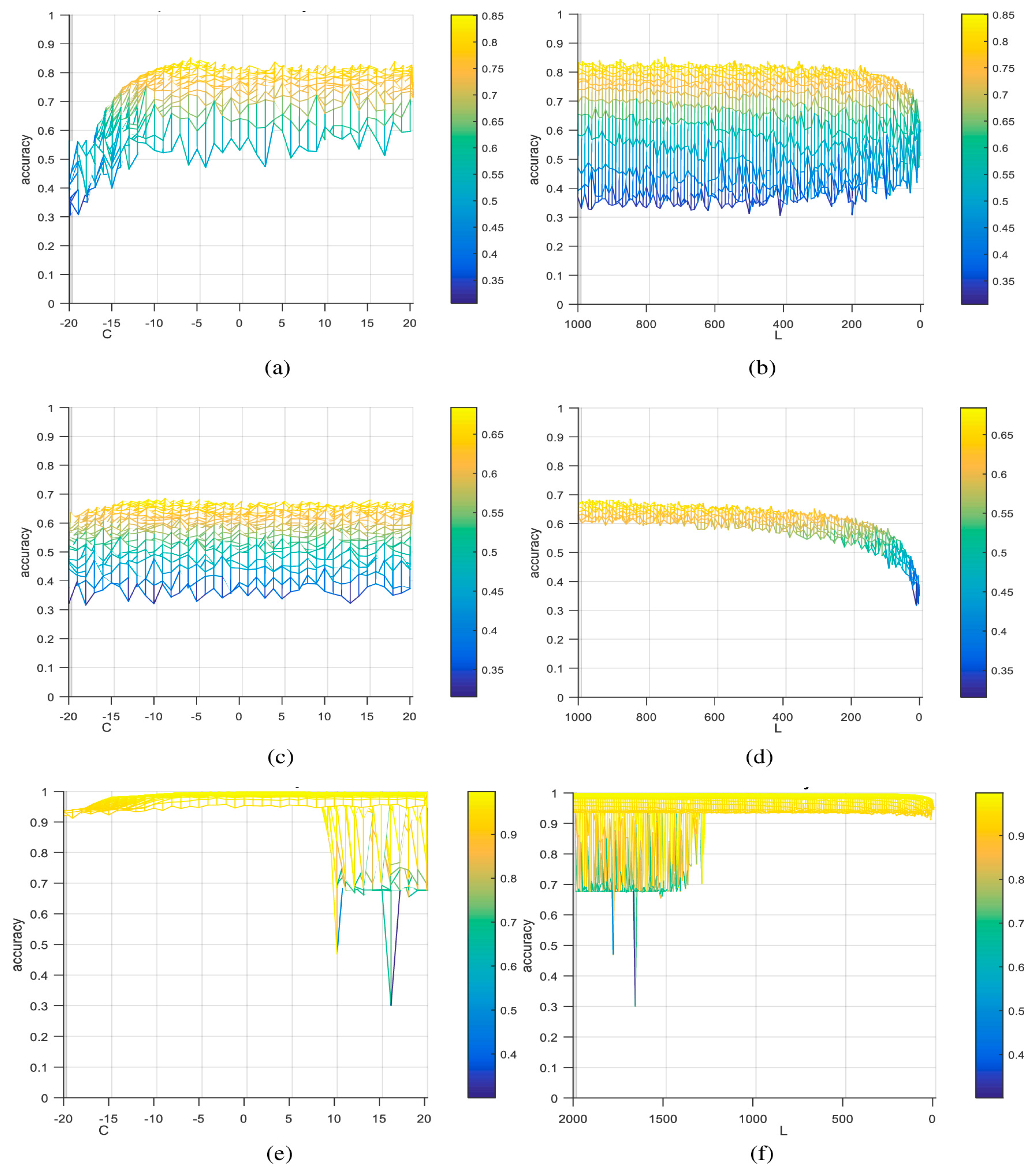
5.2. Characterization

A characterization model is required for each of the classifiers and datasets. This model aims to identify the best model settings in terms of neuron numbers, and the value of the regularization factor. To address this aim, a mesh surface was generated. Every point in the mesh represents the testing accuracy with respect to a certain value of neuron numbers and regularization factor. Figure 4 exhibits the mesh generated from each of the three datasets. Moreover, every point in the surface of the mesh had a different accuracy according to the number of hidden neurons and regularization value. The aim of this study was to select the point with the best accuracy. The regularization parameter was based on the relationship between accuracy and regularization factor (C). The number of hidden neurons was selected on the basis of their relationship with (L), which represents the number of hidden neurons.
To extract the values of C and L, the mesh was mapped to C versus the accuracy curve, or L versus the accuracy curve, respectively. The three dataset curves are shown in Figure 5, while the results for L and C that achieved the best accuracy for each of the three models are given in Table 1.

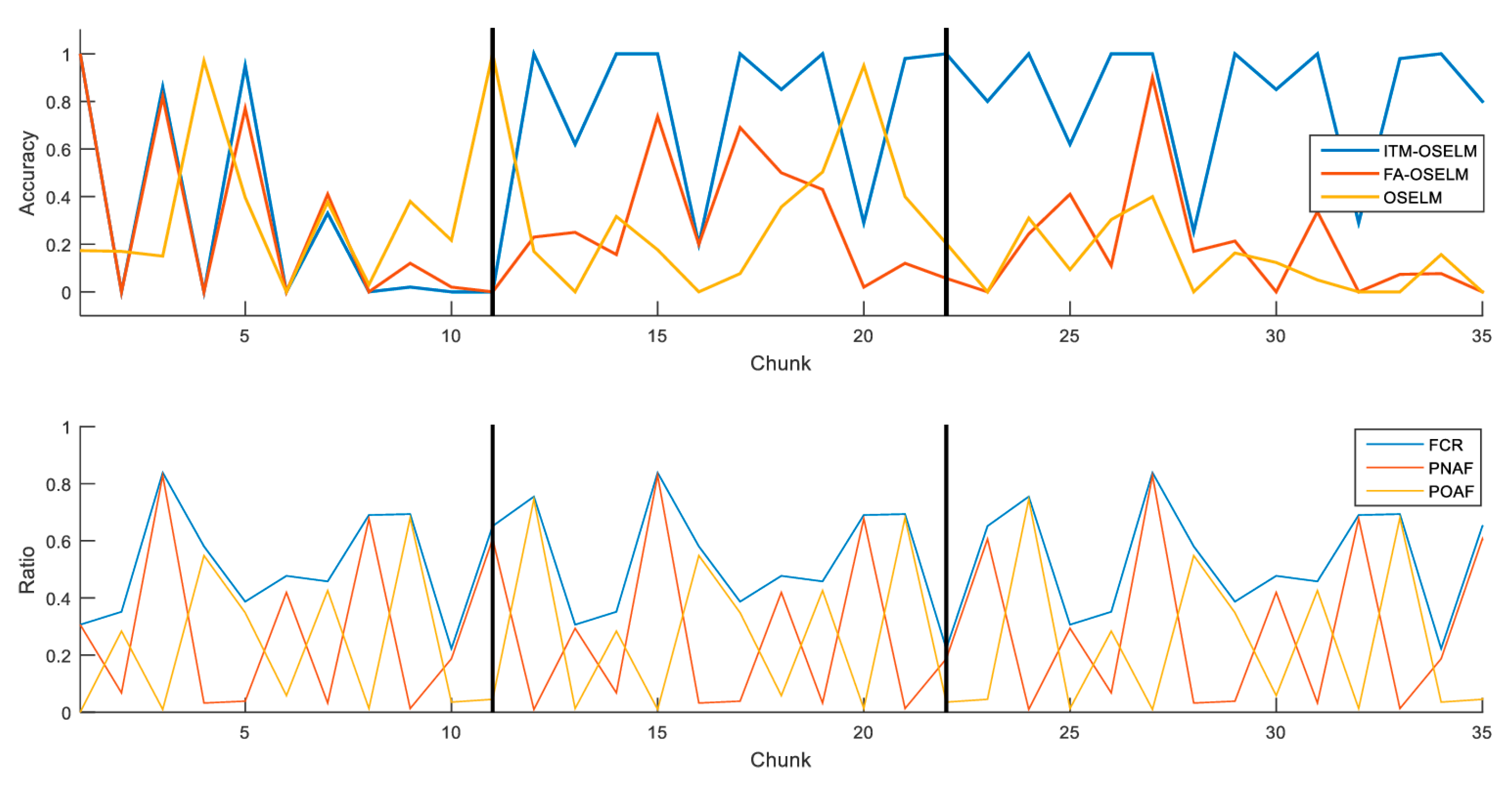
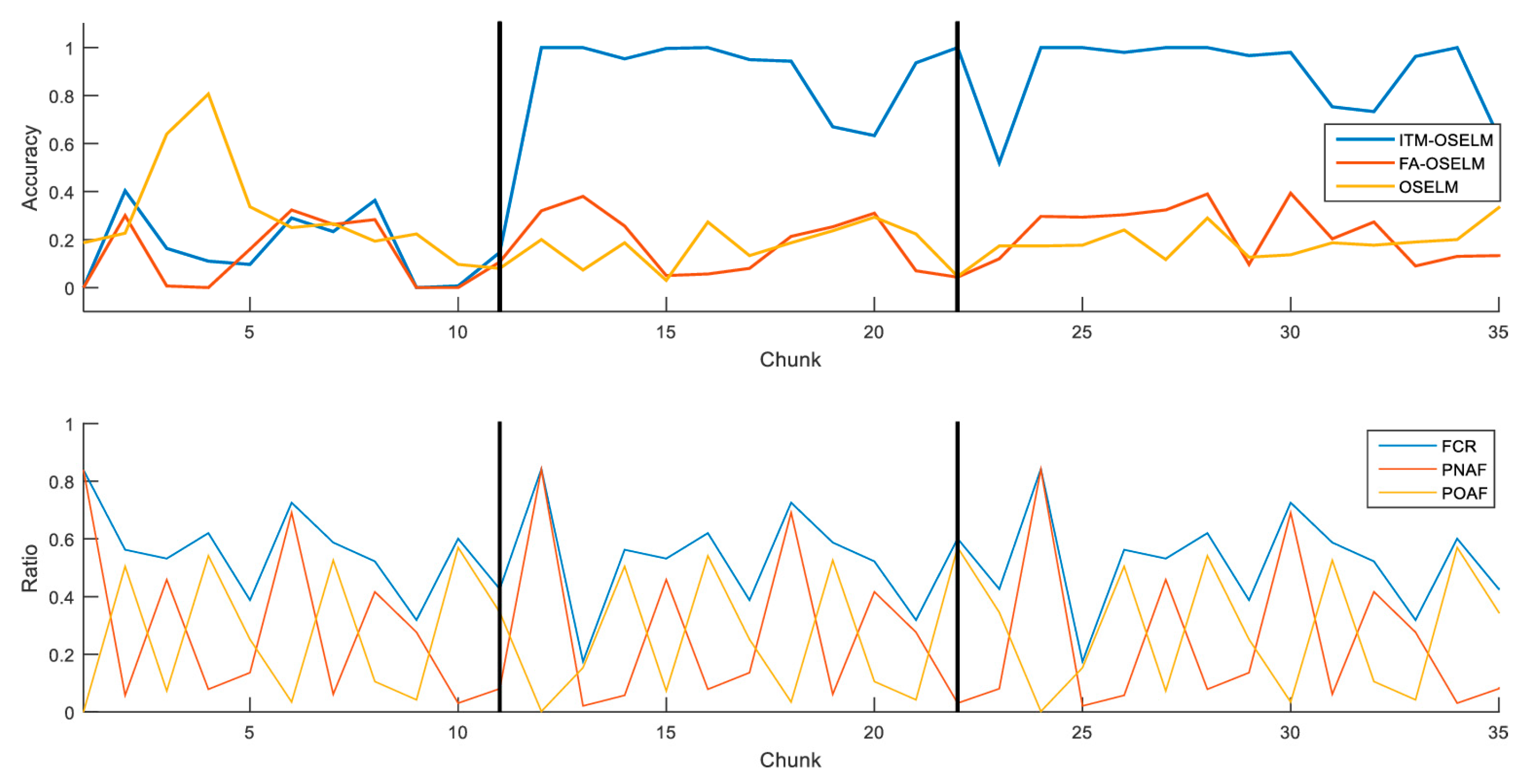
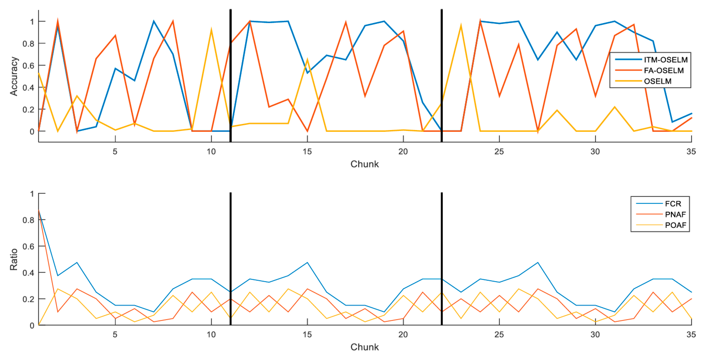
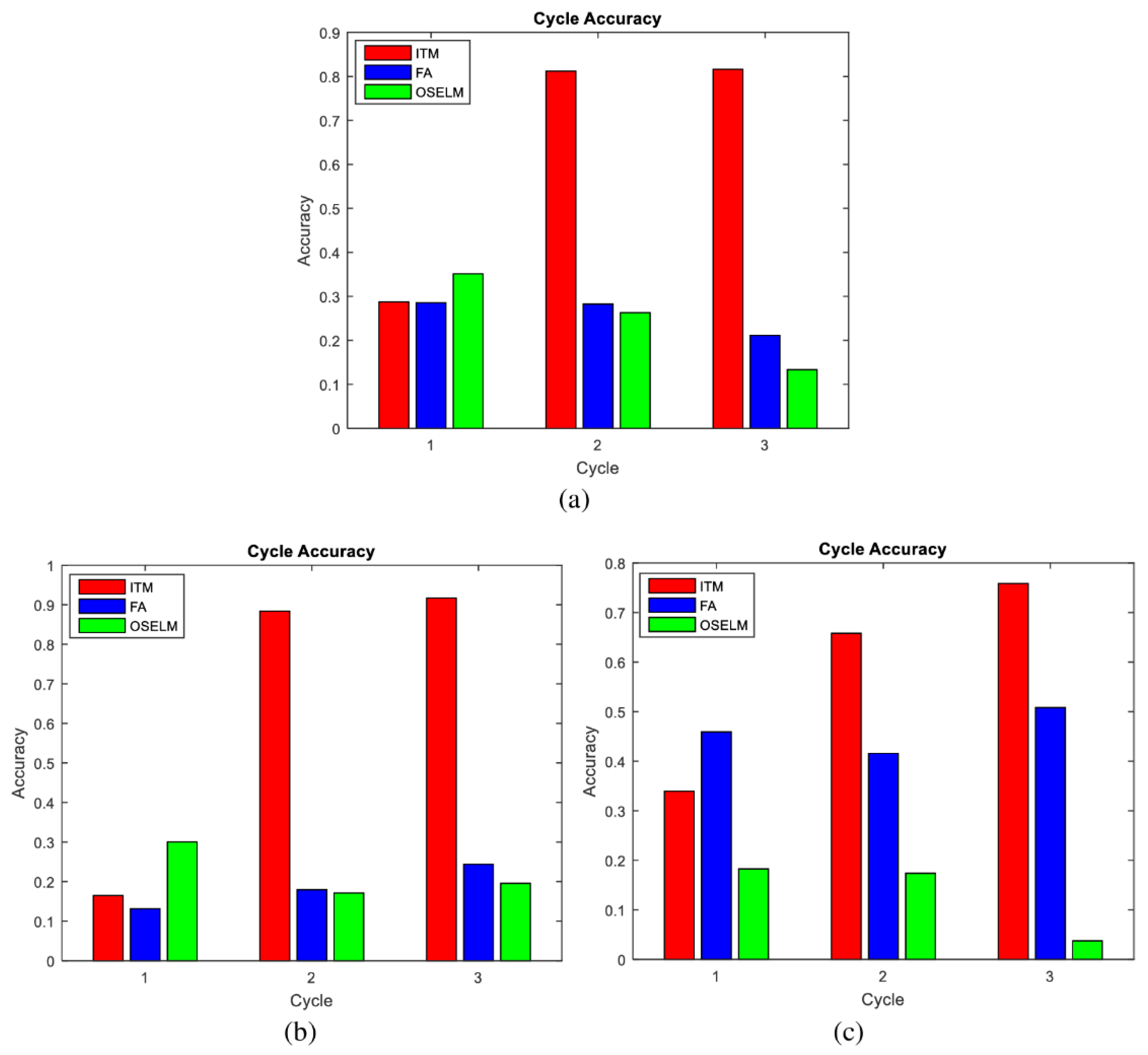
5.3. Accuracy Results

Accuracy was generated for the study’s developed model ITM-OSELM, and, for the two benchmarks, FA-OSELM and OSELM, in addition to the accuracy results. Figure 6, Figure 7, Figure 8 and Figure 9 represent the detailed accuracy with respect to chunks, and the overall accuracy in each cycle for the three datasets, respectively. Each point in the curve indicates the accuracy of one chunk in the sequential data. The chunks are coming in sequential manner because the data represents a time series data.
Analyzing the curves, for the initial cycle, the ITM-OSELM, FA-OSELM, and OSELM had similar performances because the models did not have previous knowledge to remember. In the second and third cycles, the ITM-OSELM was superior to the others, which was attributed to the comparison among their knowledge preservation aspects. FA-OSELM had transfer learning capability. However, transfer learning is a Markov type, which means it only remembers a previous state and brings its values to the current. ITM-OSELM, however, can restore older knowledge whenever necessary. On the other side, FA-OSELM and OSELM had similar performance regardless of repeating the cycle.
For further elaboration, we present Table 2, which provides the numerical values of the accuracies of each cycle for each of the three models. We observe that ITM-OSELM has achieved the highest accuracies for the three datasets in the second and third cycles. The best achieved accuracy for ITM-OSELM has been achieved in UJIndoorLoc where the overall accuracy in the third cycle was 91.69% while the accuracy of FA-OSELM and OSELM was 24.39% and 19.56%, respectively, for the third cycle. This emphasizes the superiority of ITM-OSELM over FA-OSELM and OSELM. On the other side, we observe the increase of the learning performance in ITM-OSELM when the accuracy has been increased from 16.48% in the first cycle to 88.36% in the second and 91.69% in the third cycle.
Table 3 was generated, where ITM-OSELM’s learning capability performance was quantified and compared to that of FA-OSELM and ITM-OSELM, from one cycle to another. This comparison included the learning improvement percentage during all cycles. The highest learning percentage from one cycle to another was achieved for ITM-OSELM in all three datasets; thus, ITM-OSELM was the best in terms of gaining knowledge from one cycle to another. The other two models showed negative learning rates; hence, they were not capable of carrying knowledge from one cycle to another. Moreover, the ITM-OSELM achieved better learning improvement in Cycles 2 to 1 of 182.52% compared to Cycles 3 to 1 of 0.54%, yet this improvement was not due to less capability but performance saturation as accuracy reached ~100% in the Cycle 3.
In order to validate our hypothesis of superiority of ITM-OSELM over OSELM and FA-OSELM, we adopted a t-test using a confidence level of 0.05% for rejection of H 0 of non-statistical difference in performance. In Table 4, we see in all cells of cycle 2 and cycle 3 that the values of the t-test were lower than 0.05, which means that ITM-OSELM outperforms the two baseline approaches OSELM and FA-OSELM. This proves that the reason of the superiority in the model is the transfer learning and external memory that enabled ITM-OSELM to restore old knowledge in both cycle 2 and cycle 3, while both OSELM and FA-OSELM could not do it.
In addition to accuracy, the models were evaluated according to standard machine learning evaluation measures. This evaluation was performed by selecting a class and assuming it as positive, and then the classifier was checked for any sample. The results of the classifier were either positive or negative. Figure 10, Figure 11 and Figure 12 display TP, TN, FP, or FN results. For ITM-OSELM, true measures have an increasing trend from one cycle to another, whereas false measures have a decreasing trend from one cycle to another. This discrepancy does not apply to FA-OSELM and OSELM, and the result was normal considering the accuracy results. An interesting observation is that the first cycle provides nearly similar values of TP, TN, FP and FN for all three of the models while the deviation between ITM-OSELM and the other two models occur in both the second and third cycle, which support its capability of building knowledge and achieving a higher rate of correct predictions.

6. Conclusions and Future Work

Cyclic dynamics is a common type of dynamics that occurs in time series data. Typical machine learning models are not meant to exploit learning within cyclic dynamic scenarios. In this article, we developed two concepts: first, a simulator was developed for converting datasets to time series data with changeable feature numbers or adaptive features, and for repeating the cycles of output classes; second, we developed a novel variant of the OSELM called the ITM-OSELM to deal with cyclic dynamic scenarios, and time series. The ITM-OSELM is a combination of two parts: transfer learning part, which is responsible for carrying information from one neural network to another when the number of features change; and an external memory part, which is responsible for restoring previous knowledge from old neural networks when the knowledge is needed in the current one. These models were evaluated on the basis of three datasets. The results showed that the ITM-OSELM achieved improvement in accuracy over the benchmark, where the accuracy of ITM-OSELM was 91.69%, while the accuracy of FA-OSELM and OSELM was 24.39% and 19.56% respectively.
The future work is to investigate the applicability of ITM-OSELM in various machine learning fields like video based classification or network intrusion detection. Furthermore, we will investigate the effect of the percentage of feature change in consecutive cycles on the performance of ITM-OSELM.

Author Contributions

Conceptualization, A.S.A.-K.; data curation, A.S.A.-K.; formal analysis, A.S.A.-K.; funding acquisition, M.R.A., A.A.M.I., and M.R.M.E.; investigation, A.S.A.-K. and A.A.-S.; methodology, A.S.A.-K.; project administration, A.S.A.-K. and M.H.H.; resources, A.S.A.-K. and M.H.H.; software, A.S.A.-K. and A.A.-S.; supervision, M.R.A. and A.A.M.I.; validation, M.R.A.; visualization, A.S.A.-K.; writing—original draft, A.S.A.-K.; writing—review and editing, A.S.A.-K., M.R.A., A.A.M.I., M.R.M.E., A.A.-S., and M.H.H.

Funding

This research was funded by the Malaysia Ministry of Education, Universiti Teknikal Malaysia Melaka, under Grant PJP/2018/FKEKK(3B)/S01615, and in part by the Universiti Teknologi Malaysia under Grants 14J64 and 4F966.

Conflicts of Interest

The authors declare no conflicts of interest regarding this paper.

References

  1. Zhang, J.; Liao, Y.; Wang, S.; Han, J. Study on Driving Decision-Making Mechanism of Autonomous Vehicle Based on an Optimized Support Vector Machine Regression. Appl. Sci. 2018, 8, 13. [Google Scholar] [CrossRef]
  2. Li, C.; Min, X.; Sun, S.; Lin, W.; Tang, Z. DeepGait: A Learning Deep Convolutional Representation for View-Invariant Gait Recognition Using Joint Bayesian. Appl. Sci. 2017, 7, 210. [Google Scholar] [CrossRef]
  3. Lu, J.; Huang, J.; Lu, F. Time Series Prediction Based on Adaptive Weight Online Sequential Extreme Learning Machine. Appl. Sci. 2017, 7, 217. [Google Scholar] [CrossRef]
  4. Sun, Y.; Xiong, W.; Yao, Z.; Moniz, K.; Zahir, A. Network Defense Strategy Selection with Reinforcement Learning and Pareto Optimization. Appl. Sci. 2017, 7, 1138. [Google Scholar] [CrossRef]
  5. Wang, S.; Lu, S.; Dong, Z.; Yang, J.; Yang, M.; Zhang, Y. Dual-Tree Complex Wavelet Transform and Twin Support Vector Machine for Pathological Brain Detection. Appl. Sci. 2016, 6, 169. [Google Scholar] [CrossRef]
  6. Hecht-Nielsen, R. Theory of the Backpropagation Neural Network. In Neural Networks for Perception; Harcourt Brace & Co.: Orlando, FL, USA, 1992; pp. 65–93. [Google Scholar] [CrossRef]
  7. Huang, G.-B.; Zhu, Q.-Y.; Siew, C.K. Extreme learning machine: A new learning scheme of feedforward neural networks. In Proceedings of the 2004 IEEE International Joint Conference on Neural Networks (IEEE Cat. No.04CH37541), Budapest, Hungary, 25–29 July 2004; IEEE: Piscataway, NJ, USA, 2004; Volume 2, pp. 985–990. [Google Scholar] [CrossRef]
  8. Huang, G.-B.; Liang, N.-Y.; Rong, H.-J.; Saratchandran, P.; Sundararajan, N. On-Line Sequential Extreme Learning Machine. In Proceedings of the IASTED International Conference on Computational Intelligence, Calgary, AB, Canada, 4–6 July 2005; p. 6. [Google Scholar]
  9. Jiang, X.; Liu, J.; Chen, Y.; Liu, D.; Gu, Y.; Chen, Z. Feature Adaptive Online Sequential Extreme Learning Machine for lifelong indoor localization. Neural Comput. Appl. 2016, 27, 215–225. [Google Scholar] [CrossRef]
  10. Cristianini, N.; Schölkopf, B. Support Vector Machines and Kernel Methods: The New Generation of Learning Machines. AI Mag. 2002, 23, 12. [Google Scholar] [CrossRef]
  11. Camastra, F.; Spinetti, M.; Vinciarelli, A. Offline Cursive Character Challenge: A New Benchmark for Machine Learning and Pattern Recognition Algorithms. In Proceedings of the 18th International Conference on Pattern Recognition (ICPR’06), Hong Kong, China, 20–24 August 2006; IEEE: Piscataway, NJ, USA, 2006; pp. 913–916. [Google Scholar] [CrossRef]
  12. Weiss, K.; Khoshgoftaar, T.M.; Wang, D. A survey of transfer learning. J. Big Data 2016, 3, 9. [Google Scholar] [CrossRef]
  13. Jain, V.; Learned-Miller, E. Online domain adaptation of a pre-trained cascade of classifiers. In Proceedings of the CVPR 2011, Colorado Springs, CO, USA, 20–25 June 2011; IEEE: Piscataway, NJ, USA, 2011; pp. 577–584. [Google Scholar] [CrossRef] [Green Version]
  14. Al-Khaleefa, A.S.; Ahmad, M.R.; Md Isa, A.A.; Mohd Esa, M.R.; Al-Saffar, A.; Aljeroudi, Y. Infinite-Term Memory Classifier for Wi-Fi Localization Based on Dynamic Wi-Fi Simulator. IEEE Access 2018, 6, 54769–54785. [Google Scholar] [CrossRef]
  15. Özgür, A.; Erdem, H. A review of KDD99 dataset usage in intrusion detection and machine learning between 2010 and 2015. PeerJ Prepr. 2016, 4, e1954v1. [Google Scholar] [CrossRef]
  16. Lee, W.; Stolfo, S.J. A framework for constructing features and models for intrusion detection systems. ACM Trans. Inf. Syst. Secur. 2000, 3, 227–261. [Google Scholar] [CrossRef] [Green Version]
  17. Pfahringer, B. Winning the KDD99 classification cup: Bagged boosting. ACM Sigkdd Explor. Newsl. 2000, 1, 65–66. [Google Scholar] [CrossRef]
  18. Sabhnani, M.; Serpen, G. Why Machine Learning Algorithms Fail in Misuse Detection on KDD Intrusion Detection Data Set. Intell. Data Anal. 2004, 8, 403–415. [Google Scholar] [CrossRef]
  19. Torres-Sospedra, J.; Montoliu, R.; Martinez-Uso, A.; Avariento, J.P.; Arnau, T.J.; Benedito-Bordonau, M.; Huerta, J. UJIIndoorLoc: A new multi-building and multi-floor database for WLAN fingerprint-based indoor localization problems. In Proceedings of the 2014 International Conference on Indoor Positioning and Indoor Navigation (IPIN), Busan, Korea, 27–30 October 2014; IEEE: Piscataway, NJ, USA, 2014; pp. 261–270. [Google Scholar] [CrossRef]
  20. Lohan, E.S.; Torres-Sospedra, J.; Richter, P.; Leppäkoski, H.; Huerta, J.; Cramariuc, A. Crowdsourced WiFi-fingerprinting database and benchmark software for indoor positioning. Zenodo Repos. 2017. [Google Scholar] [CrossRef]
Figure 1. Evolution of classifiers over time based on feature changes.
Applsci 09 00895 g001
Figure 2. (a) Markov model of classifier, and (b) Markov model of external memory (EM).
Applsci 09 00895 g002
Figure 3. ITM-OSELM network and its two sources of updates: external memory EM and transfer learning TL.
Applsci 09 00895 g003
Figure 4. Characterization model represented in mesh for the accuracy relation between the number of hidden neurons and regularization factor. (a) TampereU; (b) UJIndoorLoc; and (c) KDD99 datasets.
Applsci 09 00895 g004
Figure 5. Projections of the mesh on accuracy vs. regularization factor, and accuracy vs. number of neurons in hidden layers for the three datasets TampereU, UJIIndoorLoc, and KDD99. (a) Mesh representation of the relation between the accuracy, L, and C for ELM classifier based on TampereU dataset (b) relation between the accuracy and C for ELM classifier based on TampereU dataset. (c) relation between the accuracy and L for ELM classifier based on TampereU dataset. (d) relation between the accuracy, L, and C for ELM classifier based on UJIIndoorLoc dataset. (e) relation between the accuracy and C for ELM classifier based on UJIIndoorLoc dataset. (f) relation between the accuracy and L for ELM classifier based on UJIIndoorLoc dataset.
Applsci 09 00895 g005
Figure 6. Accuracy change with respect to data chunks for three cycles using the TampereU dataset.
Applsci 09 00895 g006
Figure 7. Accuracy change with respect to data chunks for three cycles using the UJIndoorLoc dataset.
Applsci 09 00895 g007
Figure 8. Accuracy change with respect to data chunks for three cycles using the KDD99 dataset.
Applsci 09 00895 g008
Figure 9. Overall accuracy for the three models with respect to cycles. (a) TampereU; (b) UJIndoorLoc; and (c) KDD99 datasets.
Applsci 09 00895 g009
Figure 10. Classification measures with respect to cycles for the three models with the TampereU dataset.
Applsci 09 00895 g010
Figure 11. Classification measures with respect to cycles for the three models with the UJIndoorLoc dataset.
Applsci 09 00895 g011
Figure 12. Classification measures with respect to cycles for the three models with the KDD99 dataset.
Applsci 09 00895 g012
Table 1. Selected values for regularization factor regularization factor (C) and number of hidden neurons (L), and their corresponding accuracy for the three datasets.
DatasetCLAccuracy
TampereU2−67500.8501
UJIndoorLoc2−98500.6841
KDD992−146000.9977
Table 2. The overall accuracy in each cycle for ITM-OSELM, FA- OSELM and OSELM in the three datasets.
DatasetAlgorithmCycle 1Cycle 2Cycle 3
TampereU datasetITM-OSELM28.73%81.17%81.61%
FA-OSELM28.55%28.25%21.11%
OSELM35.12%26.28%13.33%
UJIndoorLoc datasetITM-OSELM16.48%88.36%91.69%
FA-OSELM13.12%17.94%24.39%
OSELM30.06%17.14%19.56%
KDD99 datasetITM-OSELM33.91%65.83%75.86%
FA-OSELM45.91%41.58%50.81%
OSELM18.27%17.39%3.75%
Table 3. Learning improvement percentage of the three models with respect to cycles, percentage of the three models with respect to cycles.
DatasetAlgorithmsCycle 2 vs. Cycle 1Cycle 3 vs. Cycle 2
TampereU datasetITM-OSELM182.52%0.54%
FA-OSELM−1.05%−25.27%
OSELM−25.17%−49.27%
UJIndoorLoc datasetITM-OSELM436.16%3.76%
FA-OSELM36.73%35.95%
OSELM−42.98%14.11%
KDD99 datasetITM-OSELM94.13%15.23%
FA-OSELM−9.431%22.19%
OSELM−4.81%−78.43%
Table 4. Probabilities of the t-test for comparing ITM-OSELM with OSELM and FA-OSELM in each of the three cycles.
DatasetAlgorithms 1 vs. Algorithm 2Cycle 1Cycle 2Cycle 3
TampereU datasetITM-OSELM vs. OSELM0.731032.78 × 10−33.21 × 10⁻⁶
ITM-OSELM vs. FA-OSELM0.9342212.96 × 10−42.01 × 10⁻⁴
UJIndoorLoc datasetITM-OSELM vs. OSELM0.1260122.13 × 10−75.5 × 10⁻¹⁰
ITM-OSELM vs. FA-OSELM0.1418815.13 × 10−75.5 × 10⁻¹⁰
KDD99 datasetITM-OSELM vs. OSELM0.4224191.086 × 10−32.24 × 10⁻⁶
ITM-OSELM vs. FA-OSELM0.2995563.532 × 10−23.28 × 10⁻²

