Virtual Inertia and Mechanical Power-Based Control Strategy to Provide Stable Grid Operation under High Renewables Penetration

Abstract

This paper presents a virtual inertia and mechanical power-based control strategy to provide a stable operation of the power grid under high penetration of renewable energy sources (RESs). The proposed control technique is based on a new active and reactive power-based dynamic model with the permanent magnet synchronous generator (PMSG) swing equation, in which all PMSG features i.e., inertia and mechanical power are embedded within the controller as the main contribution of this paper. To present an accurate analysis of the virtual PMSG-based parameters, the desired zero dynamics of the grid angular frequency are considered to evaluate the effects of virtual mechanical power (VMP) on the active and reactive power sharing, as well as the investigation of virtual inertia variations for the grid angular frequency responses. Moreover, by considering various active power errors and virtual inertia, the impacts of active power error on reactive power in the proposed control technique, are precisely assessed. Simulation results are employed in Matlab/Simulink software to verify the stabilizing abilities of the proposed control technique.

1. Introduction

Emulating the behaviours of a synchronous generator (SG) in the structure of novel control techniques for power electronics converters has been increased in recent years in order to guarantee the stability of the power grid under high penetration of renewable energy sources [1,2,3,4,5,6,7].

Several studies have been reported in the literature of the modelling behaviour of SG in power electronics-based generators [8,9,10,11,12,13,14,15,16,17]. Reference [8] utilizes the concept of power hardware-in-the-loop for emulating a synchronous generator in aircraft power systems applications. A virtual synchronous generator-based control technique is presented in [12], in which the differences between inverters and real synchronous generators are considered by emulating and analysing swing and power equations [12].

Reference [13] presents a control strategy for the emulation behaviour of SG in VSC-HVDC, in which this control strategy consists of the inner and outer control loops. In addition, an inertia element is used to achieve the value of reference frequency, and a secondary frequency regulation is obtained by modulating the scheduled power in the proposed control strategy. The samples of recent research, which concentrated on modelling of power electronics-based SG emulated inertia to compensate for the lack, or low-effect, of inertia generated through conventional power plant [14]; emulated the synchronous machines for the power grid stability issues [15]; proposed an active power controller with a virtual synchronous generator that can modify inertia online [16]; and designed a virtual synchronous machine control for emulating a virtual inertia with the aim of power injection from/to the energy storage system [17].

To provide a conventional droop-based synchronous control for power electronic converters in stand-alone and grid-connected operating modes, a virtual synchronous machine-based control technique was considered in [18], by assessing the small signal responses, due to the inertia emulation characteristics. The general features of the virtual synchronous machine (VSM) are considered in [19] for smart grid applications, in which a specific VSM implementation, together with its mathematical model are discussed in the frame of numerical simulations. In order to regulate the voltage and frequency of a microgrid, a fuzzy secondary controller, based on a virtual synchronous generator is proposed for an interfaced converter in [20]. By emulating synchronous machines for the power grid stability issues, the control of HVDC transmission in [21,22,23,24] were discussed so that the used rectifier emulates the features of a synchronous motor (SM), and the applied converter mimics an SG in its control structure.

In this paper, a synchronous power controller is proposed to guarantee the desired frequency and voltage magnitude for the power grid under high penetration of renewable energy sources (RESs). After achieving an active and reactive power-based dynamic model, the virtual inertia and mechanical power parameters are incorporated in the proposed dynamic model through the PMSG swing equation, which is the main contribution of this paper. Compared to previous works, VMP variable and its error as the main effective parameters, in the proposed control technique is introduced in this paper for the first time. In addition, providing such a power-based dynamic model, along with embedding the PMSG features in this model, leads to more effective interfaced converter analogous to PMSG for providing the needed inertia that cannot found in existing methods. Then, two first and second order differential equations for the grid angular frequency are obtained that enable an accurate assessment associated with the effects of virtual mechanical power (VMP) on the active and reactive power, as well as the virtual inertia variation impacts on the grid angular frequency. To this end, the effect of active power error on the reactive power is studied. Finally, the performance of the proposed control technique is completely assessed through the simulation results.

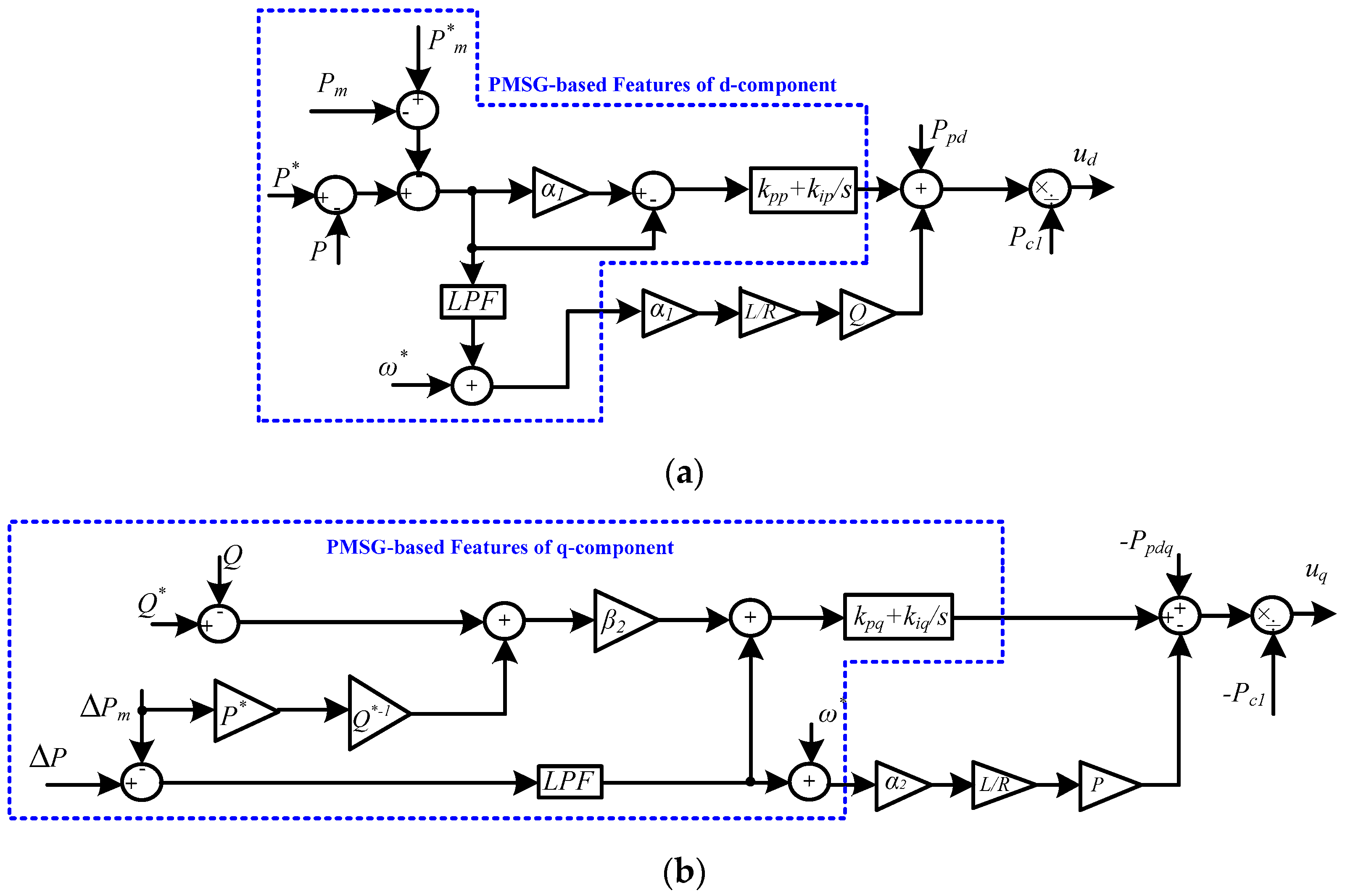
2. Introduction of the Proposed Control Technique

The general structure of the proposed model for high penetration of renewable energy sources can be seen in Figure 1. A load is connected to the power grid and a large-scale of RESs-based converters are ready for integration into power grid. The proposed controller-based converter has a duty to provide the stability for the power grid in the period of large scale integration of RESs. In this section, a new dynamic model will be extracted based on the proposed model; then, a new controller will be proposed based on the obtained dynamic model.

The Dynamic Model Analysis

To design an appropriate control technique for the control of interfaced converters, the dynamic model of the proposed model is needed. By considering the interfaced converter in Figure 1, the initial mathematical model is obtained as:

$$\begin{array}{l}L\frac{d{i}_d}{dt}+R{i}_d-\omega L{i}_q-u_d{v}_{dc}+v_d=0\\ L\frac{d{i}_q}{dt}+R{i}_q+\omega L{i}_d-u_q{v}_{dc}+v_q=0\\ C\frac{d{v}_{dc}}{dt}+u_d{i}_d+u_q{i}_q+i_{dc}=0\end{array}$$

(1)

As it is known that P = i_dv_d and Q = −i_qv_d. Considering the aforementioned relationships, (1) can be rewritten as:

$$\begin{array}{l}\frac{L}{R}\frac{dP}{dt}+P+\frac{\omega L}{R}Q-u_d{P}_{c1}+P_d=0\\ \frac{L}{R}\frac{dQ}{dt}+Q-\frac{\omega L}{R}P+u_q{P}_{c1}-P_{dq}=0\\ RC\frac{d{P}_{c1}}{dt}+u_{d}P-u_{q}Q+P_{c2}=0\end{array}$$

(2)

where, P_c1 = v_dcv_d/R, P_c2 = i_dcv_d, P_pd = v_d²/R, and P_pdq = v_dv_q/R. The PMSG swing equation is equal to:

$$J\frac{d\omega }{dt}=\frac{P_m-P}{\omega }$$

(3)

Small signal linearization is applied to (3) which leads to,

$$Js\Delta \omega =\frac{\left(\Delta P_m-\Delta P\right){\omega }^{*}-\left(P_m^{*}-P^{*}\right)\Delta \omega }{{\omega }^{*2}}$$

(4)

As a result, by the use of (4), the grid angular frequency variation is achieved as:

$$\Delta \omega =\frac{1}{{\omega }^{*}J}·\frac{\Delta P_m-\Delta P}{s+\left(P_m^{*}-P^{*}\right)/{\omega }^{*2}J}$$

(5)

The relationship (5) can be rewritten as the following,

$$\Delta P_m-\Delta P={\omega }^{*}J\left(s+\left(P_m^{*}-P^{*}\right)/{\omega }^{*2}J\right)\Delta \omega$$

(6)

Based on the active power control, the active power error relationship is driven through dividing the Laplace operator “s” by (6) as:

$$\frac{\Delta P}{s}=\frac{\Delta P_m}{s}-\left({\omega }^{*}J+\frac{\left(P_m^{*}-P^{*}\right)}{{\omega }^{*}s}\right)\Delta \omega$$

(7)

It is assumed that the interfaced converter in this paper has a nominal apparent power to generate total limited currents. It means that S = constant. Thus, by considering the relations P² + Q² = S² = constant, the relation between the small signal variables of active and reactive power can be written as,

$$2P^{*}\Delta P+2Q^{*}\Delta Q=0$$

(8)

Using Equations (7) and (8), the reactive power control-based term can be achieved as:

$$\frac{\Delta Q}{s}=-\frac{P^{*}}{Q^{*}}\frac{\Delta P_m}{s}+\frac{P^{*}}{Q^{*}}\left({\omega }^{*}J+\frac{\left(P_m^{*}-P^{*}\right)}{{\omega }^{*}s}\right)\Delta \omega$$

(9)

Equations (5), (7) and (9) are employed to design the proposed controller as:

$$\begin{array}{l}\frac{\Delta \omega }{s}=\frac{-1/{\omega }^{*}Js}{s+\left(P_m^{*}-P^{*}\right)/{\omega }^{*2}J}\Delta P+\frac{1}{{\omega }^{*}Js}·\frac{1}{s+\left(P_m^{*}-P^{*}\right)/{\omega }^{*2}J}\Delta P_m\\ \frac{\Delta P}{s}=-\left({\omega }^{*}J+\frac{\left(P_m^{*}-P^{*}\right)}{{\omega }^{*}s}\right)\Delta \omega +\frac{1}{s}\Delta P_m\\ \frac{\Delta Q}{s}=\frac{P^{*}}{Q^{*}}\left({\omega }^{*}J+\frac{\left(P_m^{*}-P^{*}\right)}{{\omega }^{*}s}\right)\Delta \omega -\frac{P^{*}}{Q^{*}}\frac{1}{s}\Delta P_m\end{array}$$

(10)

In fact, the Equation (10) is a new description of the interfaced converter that now has the PMSG characteristics included the virtual inertia, VMPE (virtual mechanical power error), and angular frequency error. According to (10), both d and q components of the proposed control technique can be drawn as Figure 2a,b. Noticing Equation (10) and Figure 2, the compensators coefficients can be stated as:

$$\begin{array}{l}{k}_{pp}={\omega }^{*}J,k_{ip}=\frac{P_m^{*}-P^{*}}{{\omega }^{*}},k_{pq}={\omega }^{*}J{P}^{*}/Q^{*}\\ k_{iq}=\frac{\left(P_m^{*}-P^{*}\right)P^{*}}{{\omega }^{*}{Q}^{*}},{\omega }_1=1/{\omega }^{*}J,{\omega }_2=\frac{P_m^{*}-P^{*}}{{\omega }^{*2}J}\end{array}$$

(11)

According to Figure 2, performance of the proposed controller is highly influenced by the embedded characteristics of PMSG that can consequently improve the controller operation with accurately regulating the virtual parameters. Also, the coefficients of α₁, α₂, β₁ and β₂ are the control factors of the proposed controller.

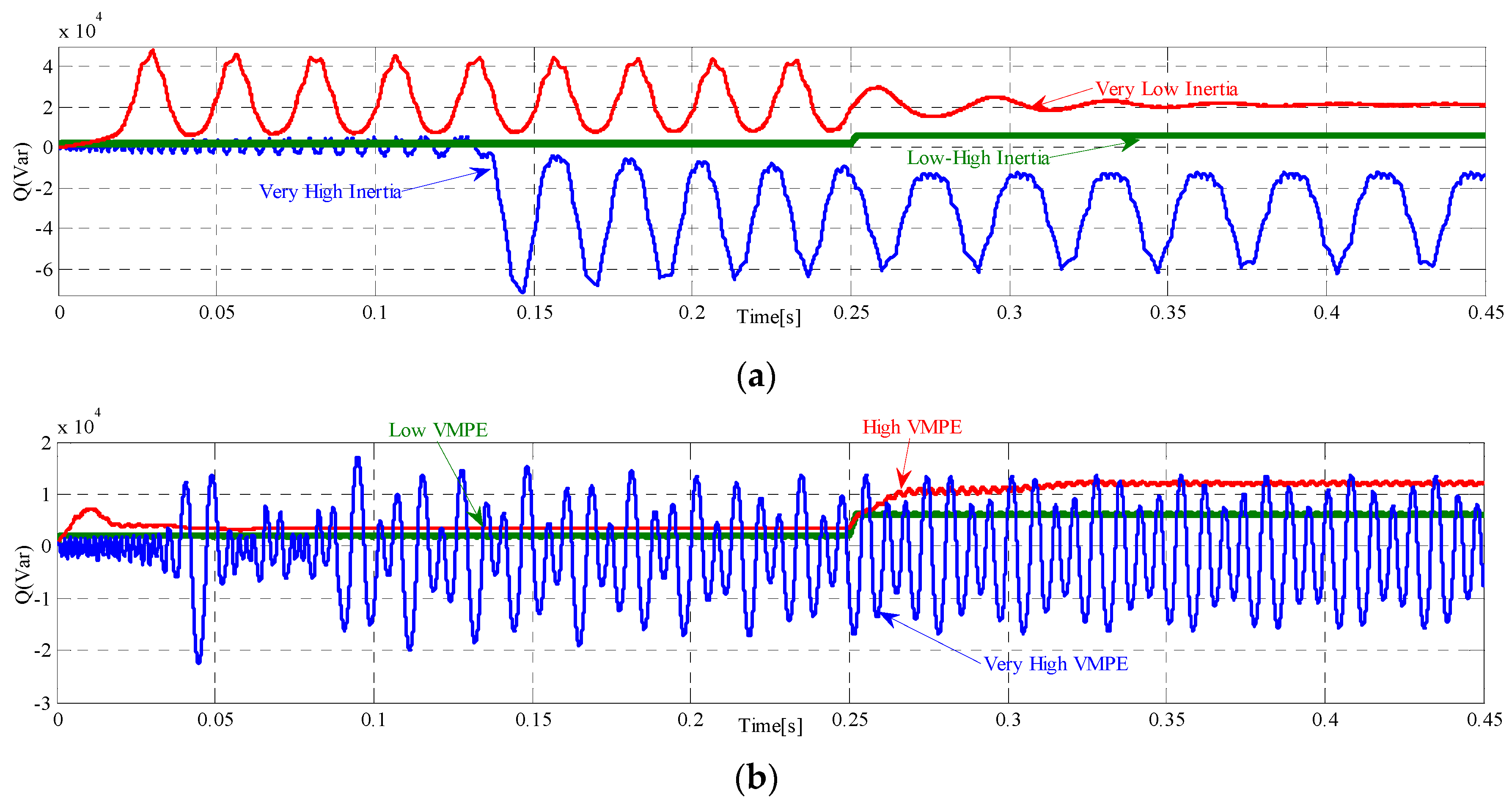
3. Evaluation the Impacts of Virtual Inertia and VMPE on the Proposed Dynamic Model

By use of the achieved active and reactive power-based dynamic model (2) along with the proposed controller-based time domain dynamic Equation (10), an evaluation related to the virtual inertia and VMPE effects is executed in this section. All power and angular frequency variations are firstly defined as:

$$\Delta x=x^{*}-xx\in \left\{P,Q,P_m,\omega \right\}$$

(12)

The time-based dynamic model of (10) can be achieved as:

$$\left({\omega }^{*2}J\right)\frac{d\omega }{dt}+\left(P_m^{*}-P^{*}\right)\omega +\left({\omega }^{*}\right)P-\left({\omega }^{*}\right)P_m=\left[{\omega }^{*2}J{\dot{\omega }}^{*}+\left(P_m^{*}-P^{*}\right){\omega }^{*}-{\omega }^{*}{P}_m^{*}+{\omega }^{*}{P}^{*}\right]$$

(13)

$$\begin{array}{l}\left({\omega }^{*2}{P}^{*}J\right)\frac{d\omega }{dt}+\left(P^{*}\left(P_m^{*}-P^{*}\right)\right)\omega -\left({\omega }^{*}{Q}^{*}\right)Q-\left({\omega }^{*}{P}^{*}\right)P_m=\\ \left[{\omega }^{*2}{P}^{*}J{\dot{\omega }}^{*}+P^{*}\left(P_m^{*}-P^{*}\right){\omega }^{*}-{\omega }^{*}{P}^{*}{P}_m^{*}-{\omega }^{*}{Q}^{*2}\right]\end{array}$$

(14)

As can be understood from (13) and (14), the zero dynamic of angular frequency i.e., dω/dt is dependent on the active power, reactive power, virtual inertia, VMP, the angular frequency, and also their reference values. Considering the desired value for dω/dt in (10) and (11) that is dω/dt = 0, the relationships (13) and (14) can be rewritten based on linear relationships for both active and reactive power as,

$$P=\left[{\omega }^{*}J{\dot{\omega }}^{*}+\left(P_m^{*}-P^{*}\right)-P_m^{*}+P^{*}\right]-\frac{\left(P_m^{*}-P^{*}\right)}{\left({\omega }^{*}\right)}\omega +P_m$$

(15)

$$Q=-\frac{\left[{\omega }^{*}{P}^{*}J{\dot{\omega }}^{*}+P^{*}\left(P_m^{*}-P^{*}\right)-P^{*}{P}_m^{*}-Q^{*2}\right]}{Q^{*}}+\frac{P^{*}\left(P_m^{*}-P^{*}\right)}{{\omega }^{*}{Q}^{*}}\omega -\frac{P^{*}}{Q^{*}}{P}_m$$

(16)

The diagrams related to (15) and (16) are drawn in Figure 3a,b, respectively. As can be seen from Figure 3a, a constant ramp is achieved for the active power diagram. The reference value increment and decrement of the VMPE can change the initial value of the active power diagram according to Figure 3a. On the other hand, as demonstrated in Figure 3b, a changeable ramp generated by varying the reactive power reference value can be observed for the reactive power diagram. Moreover, the initial value of the reactive power diagram can be altered by $P_m^{*}$ and $\Delta \omega$. These diagrams illustrate that how improved control of $P_m$ and $\omega$ can help both active and reactive power approach to desired values.

In order to reach an accurate zero dynamic-based analysis associated with the proposed controller-based model, the second order derivative of the angular frequency should be driven by use of (13) and (14) as:

$$\left({\omega }^{*2}J\right)\frac{d^2\omega }{d{t}^2}+\left(P_m^{*}-P^{*}\right)\frac{d\omega }{dt}+\left({\omega }^{*}\right)\frac{dP}{dt}=\frac{d\left[\begin{array}{l}{\omega }^{*2}J{\dot{\omega }}^{*}+\left(P_m^{*}-P^{*}\right){\omega }^{*}\\ -{\omega }^{*}{P}_m^{*}+{\omega }^{*}{P}^{*}+\left({\omega }^{*}\right)P_m\end{array}\right]}{dt}$$

(17)

$$\left({\omega }^{*2}{P}^{*}J\right)\frac{d^2\omega }{d{t}^2}+\left(P^{*}\left(P_m^{*}-P^{*}\right)\right)\frac{d\omega }{dt}-\left({\omega }^{*}{Q}^{*}\right)\frac{dQ}{dt}=\frac{d\left[\begin{array}{l}{\omega }^{*2}{P}^{*}J{\dot{\omega }}^{*}+P^{*}\left(P_m^{*}-P^{*}\right){\omega }^{*}\\ -{\omega }^{*}{P}^{*}{P}_m^{*}-{\omega }^{*}{Q}^{*2}+\left({\omega }^{*}{P}^{*}\right)P_m\end{array}\right]}{dt}$$

(18)

The zero dynamic of the VMP is found in (17) and (18). Moreover, it can be realized from (17) and (18) that the zero dynamics of the active and reactive power can highly impact on the angular frequency variations. By obtaining dP/dt and dQ/dt from the first and second terms of (2) respectively, and substituting the results into (17) and (18), two accurate zero dynamic models for the grid angular frequency with acceptable approximations can be achieved as:

$$\left({\omega }^{*2}J\right)\frac{d^2\omega }{d{t}^2}+\left(P_m^{*}-P^{*}\right)\frac{d\omega }{dt}-\left({\omega }^{*}Q\right)\omega =\left(\left(\begin{array}{l}{\omega }^{*}RP-{\omega }^{*}R{u}_d{P}_{c1}\\ +{\omega }^{*}R{P}_d\end{array}\right)/L\right)=f_1$$

(19)

$${\omega }^{*2}{P}^{*}J\frac{d^2\omega }{d{t}^2}+P^{*}\left(P_m^{*}-P^{*}\right)\frac{d\omega }{dt}-\left({\omega }^{*}{Q}^{*}P\right)\omega =\left(\left(\begin{array}{l}{\omega }^{*}{Q}^{*}RQ-{\omega }^{*}{Q}^{*}R{u}_q{P}_{c1}\\ +{\omega }^{*}{Q}^{*}R{P}_{dq}\end{array}\right)/L\right)=f_2$$

(20)

Except for the state variables involved with the converter operating conditions, both virtual inertia and mechanical power can highly impact on performance of the grid angular frequency as demonstrated in (19) and (20). By solving the differential Equations of (19) and (20), the closed-loop frequencies can be achieved as:

$$\begin{array}{l}{s}_1=\frac{-\frac{\left(P_m^{*}-P^{*}\right)}{{\omega }^{*2}J}+\sqrt{{\left(\frac{\left(P_m^{*}-P^{*}\right)}{{\omega }^{*2}J}\right)}^2+\frac{4Q}{{\omega }^{*}J}}}{2}\\ s_2=\frac{-\frac{\left(P_m^{*}-P^{*}\right)}{{\omega }^{*2}J}-\sqrt{{\left(\frac{\left(P_m^{*}-P^{*}\right)}{{\omega }^{*2}J}\right)}^2+\frac{4Q}{{\omega }^{*}J}}}{2}\end{array}$$

(21)

$$\begin{array}{l}{s}_3=\frac{-\frac{\left(P_m^{*}-P^{*}\right)}{{\omega }^{*2}J}+\sqrt{{\left(\frac{\left(P_m^{*}-P^{*}\right)}{{\omega }^{*2}J}\right)}^2+4\frac{\left(Q^{*}P\right)}{{\omega }^{*}{P}^{*}J}}}{2}\\ s_4=\frac{-\frac{\left(P_m^{*}-P^{*}\right)}{{\omega }^{*2}J}-\sqrt{{\left(\frac{\left(P_m^{*}-P^{*}\right)}{{\omega }^{*2}J}\right)}^2+4\frac{\left(Q^{*}P\right)}{{\omega }^{*}{P}^{*}J}}}{2}\end{array}$$

(22)

Considering the right-side terms of (19) and (20) and (21) and (22), the grid angular frequency can be achieved as:

$$\begin{array}{l}\omega =A+\frac{0.5f_1}{\left({\omega }^{*2}J\right)\left(\sqrt{{\left(\frac{\left(P_m^{*}-P^{*}\right)}{{\omega }^{*2}J}\right)}^2+\frac{4Q}{{\omega }^{*}J}}\right)}\left[\frac{1}{s_2}{e}^{s_{2}t}-\frac{1}{s_1}{e}^{s_{1}t}\right]+\\ \frac{0.5f_2}{{\omega }^{*2}{P}^{*}J\left(\sqrt{{\left(\frac{\left(P_m^{*}-P^{*}\right)}{{\omega }^{*2}J}\right)}^2+4\frac{\left(Q^{*}P\right)}{{\omega }^{*}{P}^{*}J}}\right)}\left[\frac{1}{s_4}{e}^{s_{4}t}-\frac{1}{s_3}{e}^{s_{3}t}\right]\end{array}$$

(23)

Various states of (23) are drawn in Figure 4. As can be seen from this figure, changing the virtual inertia can be utilized to reach a desired value for the angular frequency of grid. For positive values of s₁, s₂, s₃, and s₄, two unstable responses in Figure 4 are achieved. But in the cases of stable responses, the magnitude of fluctuations of the response is noticeably decreased as shown in Figure 4 as a blue colour. On the other hand, very low and high values of the virtual inertia can lead to the non-compensable transient reaction of the grid angular frequency. The low-high values of the virtual inertia can provide appropriate response instead. The low-high values for virtual inertia in this paper mean that the virtual inertia locates in the interval [1 × 10⁻¹ s, 1 × 10³ s]. In another word, the virtual inertia, which is smaller than 1 × 10⁻¹ s, or bigger than 1 × 10³ s, will be called very low, and high values of virtual inertia, respectively. The proposed control technique in the interval [1 × 10⁻¹ s, 1 × 10³ s] will work very well with high stability. To more understand the effects of these values, both Section 4 and Section 5 are presented.

4. Evaluation of the Impacts of Active Power Error on Reactive Power in the Proposed Controller

Reactive power sharing of the proposed controller is affected by the active power error. In this section, the reactive power operation is evaluated through the step and ramp changes of active power error, and also different values of the virtual inertia. Based on Figure 2 and Equation (2), the transfer function of reactive power and active power error can be achieved as:

$$Q/\Delta P=A_P/\Delta$$

(24)

where, A_P and Δ are given in the Appendix A. Figure 5 shows the Bode and Phase diagrams for Q/∆P, as well as the step and ramp changes of active power error around the operating angular frequency. It can be seen from the Phase diagram of Figure 5, that the Q/∆P and ramp active power error generate a phase difference of 90 degrees for the reactive power of the proposed controller. But, by carefully analysing the magnitude diagram in Figure 5, it can be achieved that the magnitude of the reactive power generated by the active power error is extremely low. To complete the aforementioned analysis, the Root Locus diagrams of reactive power for step and ramp active power error are shown in Figure 6. It can be seen from Figure 6, that a step change of active power error leads to fluctuating reactive power responses and in another case of ramp change, the reactive power becomes completely unstable as shown in Figure 6b. Changing the virtual inertia is considered in Figure 7. As it can be seen, decreasing the virtual inertia makes a little difference in the magnitude of Q/∆P related to larger value and totally for all values of the virtual inertia and the same results are approximately achieved.

5. Results and Discussions

Performance of the proposed controller in the dynamic operating condition is surveyed in this section. Also, effects of the different virtual mechanical factors including the virtual inertia and the mechanical power error are assessed. The values of simulation parameters are specified in

Table 1. Simulation parameters.

Parameter	Value	Parameter	Value
dc-link Voltage (vdc)	850 V	J1	1 × 103 s
Phase ac voltage	220 V	Pm	3.3 kW
Fundamental frequency	50 Hz	P	3 kW
Switching frequency	10 kHz	Q	2 kvar
Interface converter resistance	0.1 Ohm	Interface converter inductance	45 mH

. The general structure of the proposed controller is given in Figure 8.

5.1. Active and Reactive Power Sharing Assessment

The active and reactive power sharing ability of the proposed controller-based converter can be influenced by variation of the virtual inertia and mechanical power. Firstly, the proposed controller-based converter is supplying a 3 kW + j2 kVar grid connected load and then an abrupt disconnection of the PV sources with 4 Kw + j3 kVar occurs at the PCC at t = 0.1 s which will be supplied by the proposed controller at t = 0.25s. Figure 9 shows the active power variations under different values for virtual inertia and mechanical power.

As it can be seen from Figure 9a,b, the best response is due to the low-high values of virtual inertia as well as low VMP error. In contrast, the worst response can be achieved by very high values of both virtual inertia and mechanical power. Moreover, the active power with high VMP error is trying to follow its desired value that verifies the importance of choosing appropriately the VMP in the proposed controller. According to Figure 9a, for very low inertia, the active power reaches its reference value ultimately, however the transient takes very long time along with very high value of the transient magnitude. The reactive power of the proposed controller-based converter is illustrated in Figure 10. The same scenario associated with the best response happens for the reactive power. Also, the worst case of the reactive power response is belonging to very high value of the virtual inertia and mechanical power as shown in Figure 9a,b. In the cases of very low inertia and high VMP error, the reactive power is trying to make minimum divergence in its entire responses.

5.2. Evaluation of the Grid Frequency and the Voltage Magnitude

The same load variations are considered in this sub-section. Employing various values, for the virtual inertia and VMPE in the proposed controller, can impact on both steady stated and transient responses of the grid frequency and voltage magnitude under high renewable energy sources penetration.

The grid frequency responses, along with the virtual inertia and VMPE changes, are illustrated in Figure 11. Figure 11a shows the best response of the proposed controller for the grid frequency. According to Figure 11b, both very high and low values of the virtual inertia will lead to the worst response for the grid frequency. The grid frequency in the case of the high VMPE is making effort to remain at desired value as depicted in Figure 11c, which is in contrast to the very high values of the VMPE that leads to unstable reaction for the grid frequency. The responses of grid voltage magnitude are shown in Figure 12. Based on Figure 12a, for the appropriate values of virtual inertia and VMPE, the proposed controller is able to force the grid voltage following its reference value, with a very good transient response. The grid voltage magnitude is collapsed for both very high and low values of virtual inertia. The same scenario happens for very high VMPE and inversely the high value of VMPE can somewhat provide stable response for the grid voltage magnitude as illustrated in Figure 12c.

6. Conclusions

A control technique based on the characteristics of PMSG has been proposed in this paper to deal with the power grid stability issues under high penetration of renewable energy sources. Initially, virtual inertia and mechanical power (VMP) have been embedded in an active and reactive power-based dynamic model of the interfaced converter as the main contribution of this paper, that could provide a stable operation for the power grid, with properly varying the virtual parameters. By considering the first order zero dynamic of the grid angular frequency, the active and reactive power variations, based on VMP, have been assessed. Based on this assessment, the accurate active and reactive power sharing have been improved by appropriately controlling VMP and the error of angular frequency. Moreover, the second order zero dynamic of the grid angular frequency has been used to investigate precisely the virtual inertia effects. This investigation has shown that the stable responses of the angular frequency have driven through the so-called low-high virtual inertia. From another side, the effects of the active power error on the reactive power, under the changing virtual inertia, have been comprehensively analysed. Within the future work, authors suggest that more detailed dynamic model of PMSG can be embedded into the active and reactive power-based dynamic model, presented in this paper to design more detailed controller. Simulation results confirmed that the proposed control technique can guarantee the stability of the power grid under high penetration of renewable energy sources. The main findings of this paper are that, for a wide range of virtual inertial with VMP, stable responses with very short transient time, have been achieved for the grid frequency and voltage magnitude, as well as the active and reactive power under high penetration condition.

References

1. Ashabani, M.; Gooi, H.B.; Guerrero, J.M. Designing high-order power-source synchronous current converters for islanded and grid-connected microgrids. Appl. Energy 2017, in press. [Google Scholar] [CrossRef]
2. Vasquez-Arnez, R.L.; Ramos, D.S.; Carpio-Huayllas, T.E. Microgrid dynamic response during the pre-planned and forced islanding processes involving DFIG and synchronous generators. Int. J. Elect. Power Energy Syst. 2014, 62, 175–182. [Google Scholar] [CrossRef]
3. Mehrasa, M.; Pouresmaeil, E.; Mehrjerdi, H.; Jørgensen, B.N.; Catalão, J.P.S. Control technique for enhancing the stable operation of distributed generation units within a microgrid. Energy Convers. Manag. 2015, 97, 362–373. [Google Scholar] [CrossRef]
4. Mehrasa, M.; Adabi, M.E.; Pouresmaeil, E.; Adabi, J. Passivity based control technique for integration of DG resources into the power grid. Int. J. Elect. Power Energy Syst. 2014, 58, 281–290. [Google Scholar] [CrossRef]
5. Xiang-zhen, Y.; Jian-hui, S.; Ming, D.; Jin-wei, L.; Yan, D. Control strategy for virtual synchronous generator in microgrid. In Proceedings of the 4th International Conference on Electric Utility Deregulation and Restructing and Power Technologies DRPT, Weihai, China, 6–9 July 2011; pp. 1633–1637. [Google Scholar]
6. Mehrasa, M.; Sepehr, A.; Pouresmaeil, E.; Kyyrä, J.; Marzband, M.; Catalão, J.P.S. Angular frequency dynamic-based control technique of a grid-interfaced converter emulated by a synchronous generator. In Proceedings of the International Conference on Smart Energy Systems and Technologies IEEE Conference (SEST 2018), Sevilla, Spain, 10–12 September 2018; pp. 1–5. [Google Scholar]
7. Hasanzadeh, A.; Edrington, C.S.; Stroupe, N.; Bevis, T. Real-time emulation of a high-speed microturbine permanent-magnet synchronous generator using multiplatform hardware-in-the-loop realization. IEEE Trans. Ind. Electron. 2014, 61, 3109–3118. [Google Scholar] [CrossRef]
8. Griffo, A.; Drury, D. Hardware in the loop emulation of synchronous generators for aircraft power systems. In Proceedings of the Electrical Systems for Aircraft, Railway and Ship Propulsion ESARS, Bologna, Italy, 16–18 October 2012; pp. 1–6. [Google Scholar]
9. Pulendran, S.; Tate, J.E. Hysteresis control of voltage source converters for synchronous machine emulation. In Proceedings of the 2012 15th International Power Electronics and Motion Control Conference PEMC, Novi Sad, Serbia, 4–6 September 2012; pp. LS3b.2-1–LS3b.2-8. [Google Scholar]
10. Mehrasa, M.; Pouresmaeil, E.; Pournazarian, B.; Sepehr, A.; Marzband, M.; Catalão, J.P.S. Synchronous resonant control technique to address power grid instability problems due to high renewables penetration. Energies 2018, 11, 2469. [Google Scholar] [CrossRef]
11. Mehrasa, M.; Sepehr, A.; Pouresmaeil, E.; Marzband, M.; Catalão, J.P.S.; Kyyrä, J. Stability analysis of a synchronous generator-based control technique used in large-scale grid integration of renewable energy. In Proceedings of the 2018 International Conference on Smart Energy Systems and Technologies, IEEE Conference (SEST), Sevilla, Spain, 10–12 September 2018; pp. 1–5. [Google Scholar]
12. Li, M.; Wang, Y.; Xu, N.; Liu, Y.; Wang, W.; Wang, H.; Lei, W. A novel virtual synchronous generator control strategy based on improved swing equation emulating and power decoupling method. In Proceedings of the 2016 IEEE Energy Conversion Congress and Exposition (ECCE), Milwaukee, WI, USA, 18–22 September 2016; pp. 1–7. [Google Scholar]
13. Guan, M.; Pan, W.; Zhang, J.; Hao, Q.; Cheng, J.; Zheng, X. Synchronous generator emulation control strategy for voltage source converter (vsc) stations. IEEE Trans. Power Syst. 2015, 30, 3093–3101. [Google Scholar] [CrossRef]
14. Tielens, P.; Van Hertem, D. Influence of system wide implementation of virtual inertia on small-signal stability. In Proceedings of the 2016 IEEE International Energy Conference (ENERGYCON), Leuven, Belgium, 4–8 April 2016; pp. 1–6. [Google Scholar]
15. Aouini, R.; Marinescu, B.; Kilani, K.B.; Elleuch, M. Synchronverter-based emulation and control of hvdc transmission. IEEE Trans. Power Syst. 2016, 31, 278–286. [Google Scholar] [CrossRef]
16. Remon, D.; Cantarellas, A.M.; Rakhshani, E.; Candela, I.; Rodriguez, P. An active power self-synchronizing controller for grid-connected converters emulating inertia. In Proceedings of the 2014 International Conference on Renewable Energy Research and Application ICRERA, Milwaukee, WI, USA, 19–22 October 2014; pp. 424–429. [Google Scholar]
17. Torres, M.; Lopes, L.A.C. Virtual synchronous generator control in autonomous wind-diesel power systems. In Proceedings of the 2009 IEEE Electrical Power and Energy Conference EPEC, Montreal, QC, Canada, 22–23 October 2009; pp. 1–6. [Google Scholar]
18. Arco, S.D.; Suul, J.A. Virtual synchronous machines—classification of implementations and analysis of equivalence to droop controllers for microgrids. In Proceedings of the 2013 IEEE Grenoble Conference, PowerTech, Grenoble, France, 16–20 June 2013; pp. 1–7. [Google Scholar]
19. D’Arco, S.; Suul, J.A.; Fosso, O.B. A virtual synchronous machine implementation for distributed control of power converters in smart grids. Elec. Power Syst. Res. 2015, 122, 180–197. [Google Scholar] [CrossRef]
20. Andalib-Bin-Karim, C.; Liang, X.; Zhang, H. Fuzzy Secondary controller based virtual synchronous generator control scheme for interfacing inverters of renewable distributed generation in microgrids. IEEE Trans. Ind. Appl. 2017, 54, 1047–1061. [Google Scholar] [CrossRef]
21. Karapanos, V.; Kotsampopoulos, P.; Hatziargyriou, N. Performance of the linear and binary algorithm of virtual synchronous generators for the emulation of rotational inertia. Elec. Power. Sys. Res. 2015, 123, 119–127. [Google Scholar] [CrossRef]
22. Prieto-Araujo, E.; O-Rosell, P.; Cheah-Mañe, M.; Villafafila-Robles, R.; Gomis-Bellmunt, O. Renewable energy emulation concepts for microgrids. Renew. Sustain. Energy Rev. 2015, 50, 325–345. [Google Scholar] [CrossRef] [Green Version]
23. Bevrani, H.; Ise, T.; Miura, Y. Virtual synchronous generators: A survey and new perspectives. Int. J. Elect. Power. Energy Syst. 2014, 54, 244–254. [Google Scholar] [CrossRef]
24. Alsiraji, H.A.; El-Shatshat, R. Comprehensive assessment of virtual synchronous machine based voltage source converter controllers. IET Gener. Transm. Distrib. 2017, 11, 1762–1769. [Google Scholar] [CrossRef]
Figure 1. General structure of the high penetration renewable energy sources. RERs: Renewable Energy Sources.
Applsci 09 01043 g001
Figure 2. The proposed control technique, (a) the d-component, and (b) the q-component. PMSG: permanent magnet synchronous generator; LPF: low pass filter.
Applsci 09 01043 g002
Figure 3. Diagrams of (a) the active power based on the virtual mechanical power (VMP) with changing Pm* and Δω and (b) the reactive power based on VMP with changing Pm*, Q* and Δω.
Applsci 09 01043 g003
Figure 4. The virtual inertia effects on the grid angular frequency.
Applsci 09 01043 g004
Figure 5. Bode diagrams for Q/∆P as well as the step and ramp changes of active power error.
Applsci 09 01043 g005
Figure 6. Root Locus diagrams of reactive power in Q/∆P: (a) Step active power error and (b) ramp active power error.
Applsci 09 01043 g006
Figure 7. Various values of virtual inertia in Q/∆P.
Applsci 09 01043 g007
Figure 8. The general structure of the model based on the proposed control technique. PWM: Pulse Width Modulation; PQ: Active and Reactive Power Coordination.
Applsci 09 01043 g008
Figure 9. Active power of the proposed controller-based converter under: (a) various inertia values, and (b) various VMPE values.
Applsci 09 01043 g009
Figure 10. Reactive power of the proposed controller-based converter under: (a) various inertia values, and (b) various VMPE values.
Applsci 09 01043 g010
Figure 11. The grid frequency under (a) appropriate virtual inertia and VMPE, (b) very high and low virtual inertia, and (c) high and very high values of VMPE.
Applsci 09 01043 g011
Figure 12. The grid voltage magnitude under (a) appropriate virtual inertia and VMPE, (b) very high and low virtual inertia, and (c) high and very high values of VMPE.
Applsci 09 01043 g012