Parameterized Modeling and Planning of Distributed Energy Storage in Active Distribution Networks

Abstract

In recent years, distributed energy storage (DES) has experienced rapid growth and has been widely applied in active distribution networks (ADNs). Owing to the close correlation between the characteristics and the application scenarios, DES modeling needs to be parameterized separately for various application demands. In this paper, a parameterized model for optimal DES planning in ADNs is proposed. The typical scenarios for DES planning are generated by the clustering technique, containing the patterns of load demand, wind turbine output and photovoltaic output. Secondly, an optimal planning model of DES considering parameterized characteristics is established, which is essentially a mixed integer non-linear optimization problem. Then, the model is converted to a mixed-integer second-order cone programming model, which can be solved efficiently by available commercial software. Finally, case studies on the modified IEEE 33-node system and IEEE 123-node system verify the efficiency of the proposed method, and the effects of DES planning are validated by two evaluation indexes.

1. Introduction

With the integration of distributed generators (DGs) and flexible loads, traditional distribution systems are evolving into active distribution networks (ADNs) [1]. The integration of renewable DGs contributes to power loss reduction, power supply reliability enhancement, reduction of pollution gases emission, etc. [2,3], while bringing new challenges to the planning and operation of distribution system like voltage violation [4], bi-direction power flow [5], power flow fluctuations [6]. In recent years, distributed energy storage (DES) as an important measure to alleviate the above problems has developed rapidly in both economic and technical aspects [7,8]. Compared with large-scale centralized energy storage plants, DES has fewer restrictions on the geographical conditions of installation location and performs an increasingly important part in various application scenarios of ADNs [9].

By the criterion of discharge duration, the DES technologies can be divided into two categories, energy-type storage and power-type storage. The energy-type storage technologies, including pumped hydraulic storage (PHS), compressed air energy storage (CAES), and large-scale battery storage, are applied to provide long-term electricity support such as arbitrage [10], loss reduction [11], congestion alleviation [12], and long time-scale voltage control [13]. The latter type of energy storage, known as power-type storage, is suitable for distributed energy resources smoothing [14], power quality management [15], frequency regulation [16] and short time-scale voltage control [17]. Supercapacitor or ultracapacitor energy storage (SCES), flywheel energy storage (FES), superconducting magnetic energy storage (SMES) and small-scale battery storage belong to this category.

However, the high costs of DES, especially high investment costs, are the major obstacles limiting further development. Although some new technologies such as lead-carbon battery and LiFePO₄ (LFP) battery have largely mitigated the economic problem [18], DES is not as widely used as other traditional electricity equipment. As a result, it is of great significance to optimize the sizing and allocation of DES to maximize the economic benefits in different scenarios.

Many works in the literature have studied on the sizing and allocation of DES in ADNs. A combined genetic algorithm and sequential quadratic programming method is proposed in [19], and further testify the potential economic benefits of energy storage systems. Considering the voltage deviation, congestion, network losses and load shifting, a multi-objective planning model is proposed in [20]. A bi-level programming method is proposed in [21], and optimal planning and operation of energy storage system are solved by upper and lower programming respectively. Considering the influence of soft open point (SOP) and network configuration, a second-order cone programming (SOCP) method to determine the optimal siting and sizing DES is established in [22]. In [23], a relaxed convex optimal power flow (OPF) model is proposed, and solved by benders decomposition method. The optimal methods of resources allocation in the fields of information communication and industrial manufactory also provide ideas for DES planning. For instance, a resource service sharing model of cloud manufactory (CMfg) based on the Gale–Shapley algorithm is proposed in [24], indicating great advantages in promoting the resource-sharing utilization rate. In [25], to support the capacity sharing issue among independent firms, an advanced framework based on game theory and fuzzy logic is proposed.

The type selection of energy storage is a critical issue in DES planning [26]. The characteristics of different DES types vary in economics and technology. Owing to the close correlation between the characteristics and the application scenarios, the DES modeling needs to be parameterized separately for various application demands. For instance, low cycle efficiency will increase the cost of effective output power; and a low cycle life adds to the total cost owing to high-frequency equipment updates. A single type of energy storage device has its unique advantages, but it is difficult to incorporate high efficiency, long life, and many other requirements in one device. Therefore, coordinated planning of multiple types of energy storage systems can adequately cover the potential technical advantages of various DES, and meet the demand for energy storage performance in distribution networks. On the other hand, with the development of DES, the cost of energy storage systems will be significantly reduced, and the economic benefits in distribution networks will become more promising. For the reason that the cost of different DES types varies enormously, it is necessary to compare the costs of different types of energy storage in different scenarios and choose the optimal DES selection to maximize economic benefits. However, the quantization parameters of DES are complicated and challenging to parameterize, and it will increase the difficulty of the calculation due to the parameter multiplication of various DES types. In summary, there is a need to propose a parameterized model, which can transform the efficiency, life cycle, and other characteristics of multiple DES types into parameterized representation. The parameterized model will provide a quantitative description for different typed of DES, making it possible to scientifically and comprehensively consider the specific characteristics of different DES types in optimal planning.

This paper proposes a parameterized model for optimal DES planning in ADNs. The main contributions are summarized as follows:

(1)

The economic and technical characteristics of DES are comprehensively categorized and analyzed. Then, the influences of DES characteristics on the operation and planning are also considered to provide a parameterized modeling for DES planning in ADNs.

(2)

An optimal planning model of DES considering parameterized characteristics of DES is proposed in this paper. The proposed model considers multiple types of DES, which can solve the problem with coordinated planning. By applying the convex relaxation technique and introducing the relevant auxiliary variables, the proposed model is transformed into an effectively solved mixed-integer second-order cone programming (MISOCP) model.

The remainder of this paper is organized as follows. In Section 2, a set of parameterized data is defined to apply in DES planning in ADNs. In Section 3, considering two different application scenarios for DES, the parameterized modeling of DES planning in ADNs is proposed. Section 4 proposes the method that transforms the original model into an effectively solved mixed-integer second-order cone programming (MISOCP) model. In Section 5, numerical results on the modified IEEE 33-node system and modified IEEE 123-node system demonstrate the effectiveness of the proposed method, and the effects of DES are evaluated by two evaluation indexes. Finally, conclusions are drawn in Section 6.

2. Parameterized Representation of Distributed Energy Storage (DES) Characteristics

In general, DES normally exhibits different economic and technical characteristics [27]. The common characteristics of energy storage are the capital cost of DES, lifetime in cycles and years, power/energy density, and maximum depth of discharge (DoD). The investment cost of DES includes the cost of energy storage and power inverters, which is the most important factor affecting the economic benefits of DES. The cycle efficiency indicates the round-trip efficiency in one cycle operation. Low cycle efficiency will increase the cost of effective output power, further increasing the total energy purchase cost from the external grid. Maximum depth of discharge is the ability to discharge the total energy of DES in a discharge duration. High DoD means a higher total energy output at the same energy capacity. Meanwhile, DES with high DoD is more economical on the same capacity of total energy output. The lifetime demonstrates the durability of DES. Low cycle life will result in quickly life decreasing during the frequent switching of discharge-charge state and add to the total cost owing to high-frequency equipment updates. Overall, the characteristics of DES largely affect the results of DES planning. Therefore, all these characteristics of DES need to be taken into account and parameterized while modeling.

In this paper, three representative types of DES are considered, and the parameters are shown in

Table 1. Typical parameters of distributed energy storage (DES) [7,10].

Parameter	Lead-Acid Battery	Li-Ion Battery	VRB
Capital cost of power converter ($/kW)	50	50	50
Capital cost of energy storage ($/kWh)	125	200	250
Cycle efficiency (%)	90	95	75
Cycle life (cycles)	3000	5000	10,000
Lifetime (years)	10	12	15
Maximum depth of discharge (%)	70	90	70

[7,10]. The three types of DES have their own features: a lead-acid battery is the most widely used rechargeable battery owing to its low investment cost; a Li-ion battery has the highest efficiency; and a vanadium redox flow battery (VRB) has an exceptionally long lifetime. As a consequence, parametrized modeling is needed to search their applicability in different demand scenarios.

3. Parameterized Modeling of Optimal DES Planning in Active Distribution Networks (ADNs)

3.1. Typical Scenario Generation

By clustering techniques, the method is developed to capture the daily patterns of load demand, wind turbine output and photovoltaic output. With the clustering method, typical scenarios and their occurrence probabilities can be obtained [28]. The purpose of clustering is to group the data objects into multiple clusters in regards to the similarity. The objects within a cluster are similar, whereas the objects of different clusters are dissimilar.

The k-means algorithm is one of the most popular clustering techniques in the fields of mathematical statistics, pattern recognition, machine learning and data mining. It can well reflect the geometric and statistical significance of clustering [29].

The calculation steps of the k-means clustering algorithm are as follows:

Step 1: Given the number of clusters x, randomly select x objects from the cluster data as cluster centers;

Step 2: According to the principle that the distance from the cluster center is the smallest, the remaining objects are assigned to the corresponding categories;

Step 3: After all the objects are divided by category, the cluster center is recalculated; the object with the smallest sum of distances to other objects in the same category is determined as the center of the current class;

Step 4: Repeat Steps (2) and (3) until the cluster center no longer changes, the cluster ends. Then, the clustering result is obtained.

By the above steps, the typical scenarios for DES planning are generated by the clustering technique, containing the patterns of load demand, wind turbine output and photovoltaic output.

3.2. Objective Function

In order to clearly show the feasibility and applicability of the proposed method in different application scenarios, two objective functions are considered and calculated respectively. Moreover, to meet the comprehensive planning requirements in real scenarios, the individual objects can be easily combined and solved by the multi-objective approaches.

In reality, the DGs and DES may have different ownerships, such as belonging to the distribution company, the third-party, and the consumers. The differences in ownerships may affect their observability, controllability, and dispatch cost. For simplicity, all the DGs and DES in this paper are assumed to be owned by the distribution company or the distribution system operator (DSO), which means that they all can be dispatched without extra costs besides the operational cost. The dispatch cost of DGs that belong to the third-party can be easily considered in the proposed method with an additional cost item.

3.2.1. Economic Benefits of ADN

The minimum annual comprehensive cost of ADN is set as the objective function, which is expressed as follows:

$$\min C_1=C^{\mathrm{OPE}}+C^{\mathrm{INV}}$$

(1)

where $C^{\mathrm{OPE}}$ is the annual operation cost of ADN and $C^{\mathrm{INV}}$ is the investment cost of DES, which are formulated as follows:

$$C^{\mathrm{OPE}}={{\displaystyle \sum }}_{s\in {\mathsf{\Omega }}_{\mathrm{S}}}\left({{\displaystyle \sum }}_{t\in N_{\mathrm{T}}}{\lambda }_t{P}_{s,t}^{\mathrm{SUB}}\Delta t\right)p_s$$

(2)

$$C^{\mathrm{INV}}=\frac{d{(1+d)}^{y_m}}{{(1+d)}^{y_m}-1}{{\displaystyle \sum }}_{m\in {\mathsf{\Omega }}_{\mathrm{type}}}{{\displaystyle \sum }}_{i\in N_{\mathrm{N}}}\left(C_m^{\mathrm{POW}}{y}_{i,m}{S}_m^{\mathrm{unit}}+C_m^{\mathrm{ENE}}{z}_{i,m}{E}_m^{\mathrm{unit}}\right)$$

(3)

where ${\mathsf{\Omega }}_{\mathrm{S}}$ is the set of scenarios and ${\mathsf{\Omega }}_{\mathrm{type}}$ is the set of DES types. $N_{\mathrm{T}}$ is the total periods of the time horizon. $N_{\mathrm{N}}$ is the total number of the nodes. $C_m^{\mathrm{POW}}$ and $C_m^{\mathrm{ENE}}$ are the capital cost for 1 kW power capacity and 1 kWh energy capacity of the $m\mathrm{th}$ DES. $S_m^{\mathrm{unit}}$ and $E_m^{\mathrm{unit}}$ are the unit power capacity and energy capacity of the $m\mathrm{th}$ DES. $y_{i,m}$ and $z_{i,m}$ are the total number of power units and energy units of the $m\mathrm{th}$ DES at node $i$. $P_{s,t}^{\mathrm{SUB}}$ is the active power at the substation in the $s\mathrm{th}$ scenario. $\Delta t$ is the time interval, ${\lambda }_t$ is the time-of-use electricity price, $p_s$ is the probability of the $s\mathrm{th}$ scenario, $d$ is the discount rate of DES, and $y_m$ is the lifetime of the $m\mathrm{th}$ DES.

The annual operation cost of an ADN is represented by the cost of total energy purchasing from the external grid under the electricity time-of-use tariff. The benefits brought by DES in power loss reduction can be reflected in the cost of energy purchasing from the external grid. The investment cost includes the cost of energy storage and power inverter.

As the power source of the distribution network, the substation node can be conveniently equipped with DES to optimize the power flow between the distribution network and the external bulk power grid. However, in this paper we mainly focus on the optimization within the distribution network by the optimal planning of different DESs. For this application, the effectivity of DES that installed at the source node is limited. Therefore, all the nodes except the substation node are considered as candidate locations for DES planning in this paper.

3.2.2. Power Fluctuation Smoothing

Utilizing the fast charge/discharge characteristics, DES can effectively smooth the rapid power fluctuation brought by renewable DGs comprising wind turbines (WTs) and photovoltaic generators (PVs). Considering the investment cost of DES and the ability to smooth power fluctuation of DGs, the objective function is expressed as follows:

$$\min C_2={\lambda }_f{C}^{\mathrm{FLU}}+C^{\mathrm{INV}}$$

(4)

where ${\lambda }_f$ is the cost of DG power fluctuation. To demonstrate the performance of DES in the application scenario of power fluctuation smoothing, ${\lambda }_f$ is the transformed parameter indicating the mathematical relationship between the power fluctuation and the investment cost of DES. The purpose of the transformation process is to make the objective function more clear. ${\lambda }_f$ is designed according to [30]. $C^{\mathrm{FLU}}$ is the power fluctuation of DG, which is expressed as:

$$C^{\mathrm{FLU}}={{\displaystyle \sum }}_{s\in {\mathsf{\Omega }}_{\mathrm{S}}}\left\{{{\displaystyle \sum }}_{m\in {\mathsf{\Omega }}_{\mathrm{type}}}{{\displaystyle \sum }}_{i\in N_{\mathrm{N}}}{{\displaystyle \sum }}_{t\in N_{\mathrm{T}}}{\left[\left(P_{s,t,i}^{\mathrm{DG}}+P_{s,t,i,m}^{\mathrm{DES}}\right)-\left(P_{s,t-1,i}^{\mathrm{DG}}+P_{s,t-1,i,m}^{\mathrm{DES}}\right)\right]}^2\right\}{p}_s$$

(5)

where $P_{s,t,i}^{\mathrm{DG}}$ is the active power injection by DG at node $i$ in the $s\mathrm{th}$ scenario, and $P_{s,t,i,m}^{\mathrm{DES}}$ is the active power injection by the $m\mathrm{th}$ DES at node $i$ in the $s\mathrm{th}$ scenario.

The power fluctuation of DG is determined by the accumulation of power difference between adjacent moments. Considering that the DES integrated with DGs can be best utilized to smooth the power fluctuation, only the nodes with DG installed are considered as candidate locations for DES planning in this application scenario.

3.3. System Power Flow Constraint

$${{\displaystyle \sum }}_{ik\in {\mathsf{\Omega }}_{\mathrm{b}}}{P}_{s,t,ik}={{\displaystyle \sum }}_{ji\in {\mathsf{\Omega }}_{\mathrm{b}}}\left(P_{s,t,ji}-r_{ji}{I}_{s,t,ji}^2\right)+P_{s,t,i}$$

(6)

$${{\displaystyle \sum }}_{ik\in {\mathsf{\Omega }}_{\mathrm{b}}}{Q}_{s,t,ik}={{\displaystyle \sum }}_{ji\in {\mathsf{\Omega }}_{\mathrm{b}}}\left(Q_{s,t,ji}-x_{ji}{I}_{s,t,ji}^2\right)+Q_{s,t,i}$$

(7)

$$P_{s,t,i}=P_{s,t,i}^{\mathrm{DG}}+{{\displaystyle \sum }}_{m\in {\mathsf{\Omega }}_{\mathrm{type}}}{P}_{s,t,i,m}^{\mathrm{DES}}-P_{s,t,i}^{\mathrm{LOAD}}$$

(8)

$$\begin{array}{c}{Q}_{s,t,i}=Q_{s,t,i}^{\mathrm{DG}}+{{\displaystyle \sum }}_{m\in {\mathsf{\Omega }}_{\mathrm{type}}}{Q}_{s,t,i,m}^{\mathrm{DES}}-Q_{s,t,i}^{\mathrm{LOAD}}\end{array}$$

(9)

$$P_{s,t}^{\mathrm{SUB}}={{\displaystyle \sum }}_{ij\in {\mathsf{\Omega }}_{\mathrm{b}}}{P}_{s,t,ij}, i\in {\mathsf{\Omega }}_{\mathrm{sub}}$$

(10)

$$U_{s,t,i}^2-U_{s,t,j}^2-2\left(r_{ij}{P}_{s,t,ij}+x_{ij}{Q}_{s,t,ij}\right)+\left(r_{ij}^2+x_{ij}^2\right)I_{s,t,ij}^2=0$$

(11)

$$I_{s,t,ij}^2=\frac{P_{s,t,ij}^2+Q_{s,t,ij}^2}{U_{s,t,i}^2}$$

(12)

where ${\mathsf{\Omega }}_{\mathrm{b}}$ is the set of all branches and ${\mathsf{\Omega }}_{\mathrm{sub}}$ is the set of substation nodes. $P_{s,t,ij}$ and $Q_{s,t,ij}$ are the active and reactive power flow of branch $ij$ in the $s\mathrm{th}$ scenario. $P_{s,t,i}$ and $Q_{s,t,i}$ are the total active and reactive power injection at node $i$ in the $s\mathrm{th}$ scenario. $I_{t,ij}$ is the branch current magnitude and $U_{t,i}$ is the node voltage magnitude. $r_{ij}$ and $x_{ij}$ are the resistance and reactance of branch $ij$. $P_{s,t,i}^{\mathrm{LOAD}}$ and $Q_{s,t,i}^{\mathrm{LOAD}}$ is the active and reactive power load at node $i$ in the $s\mathrm{th}$ scenario.

Constraints (6) and (7) represent the power balance of node $i$ in period $t$ at the $s\mathrm{th}$ scenario. The power injection of node $i$ in period $t$ in the $s\mathrm{th}$ scenario can be described as (8) and (9). Constraint (10) represents the active power balance at the substation node. The voltage drop equation over each branch is expressed as (11). The current magnitude of each branch can be determined by using (12).

3.4. Secure Operation Constraint

$${\left(U_i^{\min }\right)}^2\le U_{s,t,i}^2\le {\left(U_i^{\max }\right)}^2$$

(13)

$$0\le I_{s,t,ij}^2\le {\left(I_{ij}^{\max }\right)}^2$$

(14)

where $U_i^{\min }$ and $U_i^{\max }$ are the lower and upper limit of statutory voltage at node $i$. $I_{ij}^{\max }$ is the upper limit of statutory current at branch $ij$. The limits on nodal voltage and current are described as constraints (13) and (14).

3.5. DES Operation Constraint

$$\sqrt{{(P_{s,t,i,m}^{\mathrm{DES}})}^2+{(Q_{s,t,i,m}^{\mathrm{DES}})}^2}\le y_{i,m}{S}_m^{\mathrm{unit}}$$

(15)

$$P_{s,t,i,m}^{\mathrm{DES},\mathrm{L}}=A_m^{\mathrm{DES}}\sqrt{{(P_{s,t,i,m}^{\mathrm{DES}})}^2+{(Q_{s,t,i,m}^{\mathrm{DES}})}^2}$$

(16)

$$E_{s,t+\Delta t,i,m}^{\mathrm{DES}}=E_{s,t,i,m}^{\mathrm{DES}}-\left(P_{s,t,i,m}^{\mathrm{DES}}+P_{s,t,i,m}^{\mathrm{DES},\mathrm{L}}\right)\Delta t$$

(17)

$$\begin{array}{c}{z}_{i,m}{E}_m^{\mathrm{unit}}SO{C}_m^{\min }\le E_{s,t,i,m}^{\mathrm{DES}}\le z_{i,m}{E}_m^{\mathrm{unit}}SO{C}_m^{\max }\end{array}$$

(18)

$$\frac{{{\displaystyle \sum }}_{t\in N_{\mathrm{T}}}\left|P_{s,t,i,m}^{\mathrm{DES}}\right|\Delta t}{2z_{i,m}{E}_m^{\mathrm{unit}}}\le \frac{1}{365}\frac{N_m^{\mathrm{M}}}{y_m}$$

(19)

$$E_{s,i,m,t=T}^{\mathrm{DES}}=z_{i,m}{E}_m^{\mathrm{unit}}SO{C}_{s,m,t=0}$$

(20)

where $P_{s,t,i,m}^{\mathrm{DES}}$ and $Q_{s,t,i,m}^{\mathrm{DES}}$ are the active and reactive power injection by the $m\mathrm{th}$ DES at node $i$ in the $s\mathrm{th}$ scenario. $E_{s,t,i,m}^{\mathrm{DES}}$ is the energy stored of the $m\mathrm{th}$ DES at node $i$ in the $s\mathrm{th}$ scenario. $A_m^{\mathrm{DES}}$ is the loss coefficient of the $m\mathrm{th}$ DES. $SO{C}_m^{\min }$ and $SO{C}_m^{\max }$ are the minimum and maximum state of charge limit of the $m\mathrm{th}$ DES. $N_m^{\mathrm{M}}$ is the cycle life of the $m\mathrm{th}$ DES.

Constraint (15) represents the converter capacity limit of DES. The power loss of DES is considered in constraint (16). Constraint (17) determines that the energy stored in DES in period $\left(t+1\right)$ depends on the previous energy stored in DES and the charge/discharge power of the time interval. Constraint (18) represents the maximum and minimum state of charge (SOC) limits. Weighted energy throughput method is adopted to describe the cycle life of DES in constraint (19) [31]. The constraint relies on the principle that an electrochemical cell can exchange a finite amount of charge during its lifespan. This value can be assessed through cycling tests and calculated as the charge that pass through a cell during a complete discharge-charge cycle multiplied by the total number of cycles that a battery can perform before depletion. Constraint (20) implies that the energy stored in DES at the end of one day has to equal its initial value. It is noteworthy that the power of DES is determined by the minimum power of the energy storage equipment and the power converter. To make the DES modeling more generalized and simplified, an ideal power matching between the energy storage device and its power converter is assumed in this paper. Therefore, constraint (15) can be considered as the power limit of the entire energy storage system.

3.6. DES Planning Constraint

$${{\displaystyle \sum }}_{m\in {\mathsf{\Omega }}_{\mathrm{type}}}{{\displaystyle \sum }}_{i\in N_{\mathrm{N}}}{y}_{i,m}{S}_m^{\mathrm{unit}}\le S^{\mathrm{BGT}}$$

(21)

$${{\displaystyle \sum }}_{m\in {\mathsf{\Omega }}_{\mathrm{type}}}{{\displaystyle \sum }}_{i\in N_{\mathrm{N}}}{z}_{i,m}{E}_m^{\mathrm{unit}}\le E^{\mathrm{BGT}}$$

(22)

$$\frac{y_{i,m}{S}_m^{\mathrm{unit}}}{S^{\mathrm{BGT}}}\le {\delta }_i$$

(23)

$$\begin{array}{c}{{\displaystyle \sum }}_{i\in N_{\mathrm{N}}}{\delta }_i\le n^{\mathrm{DES}}\end{array}$$

(24)

where $S^{\mathrm{BGT}}$ and $E^{\mathrm{BGT}}$ are the maximum power capacity and energy capacity of DES in planning. ${\delta }_i$ is a binary variable indicating the location of DES at node $i$. $n^{\mathrm{DES}}$ is the maximum number of DES installing nodes.

Constraints (21) and (22) represent the maximum limits on power and energy capacity of DES in planning. The constraint that represents whether DES is installed at node $i$ can be described as (23). When ${\delta }_i=1$, DES is installed at node $i$; when ${\delta }_i=0$, no DES is installed at node $i$. The limit on the maximum number of nodes that DES can be installed is expressed as constraint (24).

As a consequence, parameterized model for optimal DES planning in ADN is finally expressed as (25), which is a mixed-integer non-linear programming (MINLP) model.

$$\begin{gathered} \mathrm{MINLP}\mathrm{Model}:\min C_1\mathrm{or}\min C_2 \\ \mathrm{s}.\mathrm{t}.\left(6\right)–\left(24\right) \end{gathered}$$

(25)

4. Mixed-Integer Second-Order Cone Programming (MISOCP) Model Conversion

In this section, to solve the MINLP model more effectively, the original model is converted into a MISOCP model by convex relaxation. First, let $u_{s,t,i}$ and $i_{s,t,ij}$ denote the quadratic terms $U_{s,t,i}^2$ and $I_{s,t,ji}^2$ Linearized functions are expressed as follows:

$${{\displaystyle \sum }}_{ik\in {\mathsf{\Omega }}_{\mathrm{b}}}{P}_{s,t,ik}={{\displaystyle \sum }}_{ji\in {\mathsf{\Omega }}_{\mathrm{b}}}\left(P_{s,t,ji}-r_{ji}{i}_{s,t,ij}\right)+P_{s,t,i}$$

(26)

$${{\displaystyle \sum }}_{ik\in {\mathsf{\Omega }}_{\mathrm{b}}}{Q}_{s,t,ik}={{\displaystyle \sum }}_{ji\in {\mathsf{\Omega }}_{\mathrm{b}}}\left(Q_{s,t,ji}-x_{ji}{i}_{s,t,ij}\right)+Q_{s,t,i}$$

(27)

$$u_{s,t,i}-u_{s,t,j}-2\left(r_{ij}{P}_{s,t,ij}+x_{ij}{Q}_{s,t,ij}\right)+\left(r_{ij}^2+x_{ij}^2\right)i_{s,t,ij}=0$$

(28)

$$i_{s,t,ij}=\frac{P_{s,t,ij}^2+Q_{s,t,ij}^2}{u_{s,t,i}}$$

(29)

$${\left(U_i^{\min }\right)}^2\le u_{s,t,i}\le {\left(U_i^{\max }\right)}^2$$

(30)

$$0\le i_{s,t,ij}\le {\left(I_{ij}^{\max }\right)}^2$$

(31)

The operation constraints of DES in (15) and (16) can be transformed into the rotated quadratic cone constraints:

$${\left(P_{s,t,i,m}^{\mathrm{DES}}\right)}^2+{\left(Q_{s,t,i,m}^{\mathrm{DES}}\right)}^2\le 2\frac{y_{i,m}{S}_m^{\mathrm{unit}}}{\sqrt{2}}\frac{y_{i,m}{S}_m^{\mathrm{unit}}}{\sqrt{2}}$$

(32)

$${\left(P_{s,t,i,m}^{\mathrm{DES}}\right)}^2+{\left(Q_{s,t,i,m}^{\mathrm{DES}}\right)}^2\le 2\frac{P_{s,t,i,m}^{\mathrm{DES},\mathrm{L}}}{\sqrt{2}{A}_m^{\mathrm{DES}}}\frac{P_{s,t,i,m}^{\mathrm{DES},\mathrm{L}}}{\sqrt{2}{A}_m^{\mathrm{DES}}}$$

(33)

Although the absolute value term $\left|P_{s,t,i,m}^{\mathrm{DES}}\right|$ in constraint (19) is nonlinear, it can be replaced by a linear program according to Chebyshev approximation problem [32]. An auxiliary variable $P_{s,t,i,m}^{\mathrm{AUX}}$ is introduced to replace $\left|P_{s,t,i,m}^{\mathrm{DES}}\right|$, and constraint (19) can be transformed to constraint (34). Constraints (35)–(37) are added to bound the value of $P_{s,t,i,m}^{\mathrm{AUX}}$, making constraint (34) linearized. Then, the constraint (19) is transformed into constraints (34)–(37), which are expressed as:

$$\frac{{{\displaystyle \sum }}_{t\in N_{\mathrm{T}}}{P}_{s,t,i,m}^{\mathrm{AUX}}\Delta t}{2z_{i,m}{E}_m^{\mathrm{unit}}}\le \frac{1}{365}\frac{N_m^{\mathrm{M}}}{y_m}$$

(34)

$$P_{s,t,i,m}^{\mathrm{AUX}}\ge P_{s,t,i,m}^{\mathrm{DES}}$$

(35)

$$P_{s,t,i,m}^{\mathrm{AUX}}\ge -P_{s,t,i,m}^{\mathrm{DES}}$$

(36)

$$P_{s,t,i,m}^{\mathrm{AUX}}\ge 0$$

(37)

Constraint (29) is relaxed to the inequality constraint (38), then transformed into second-order cone constraint (39) [33]:

$$P_{s,t,ij}^2+Q_{s,t,ij}^2\le i_{s,t,ij}{u}_{s,t,i}$$

(38)

$$\left|\right|{\left[\begin{array}{ccc}2P_{s,t,ij}& 2Q_{s,t,ij}& i_{s,t,ij}-u_{s,t,i}\end{array}\right]}^{\mathrm{T}}{\left|\right|}_2\le i_{s,t,ij}+u_{s,t,i}$$

(39)

After the conic relaxation, the original MINLP model is converted into a MISOCP model to realize an efficient calculation. The MISOCP model is expressed as:

$$\begin{gathered} \mathrm{MISOCP}\mathrm{Model}:\min C_1\mathrm{or}\min C_2 \\ \mathrm{s}.\mathrm{t}.\left(8\right)–\left(10\right),\left(17\right),\left(18\right),\left(20\right)–\left(24\right),\left(26\right)–\left(28\right),\left(30\right)–\left(37\right),\left(39\right) \end{gathered}$$

(40)

5. Case Study

In this section, the effectiveness of the proposed method is analyzed and verified on a modified IEEE 33-node system [34]. The voltage level is 12.66 kV, the total active load is 3715 kW, and the total reactive load is 2300 kvar. The test case is shown in Figure 1.

Three types of DES are available to be selected in the planning, and the parameters are shown in Table 1. Five wind turbines and three photovoltaic generators are installed, as shown in

Table 2. Parameters of distributed generators (DGs).

Parameter	Wind Turbines					Photovoltaic Generators
Location	10	16	17	30	33	7	13	27
Capacity (kVA)	500	300	200	200	300	500	300	400

. The investment costs of DES are annualized based on a discount rate of 8%. Time-of-use electricity price is shown in

Table 3. Parameters of time-of-use electricity price.

Parameter	On-Peak	Mid-Peak	Off-Peak
Time span	16:00–22:00	8:00–15:00	1:00–7:00, 23:00–24:00
Electricity price ($/kWh)	0.173	0.104	0.050

.

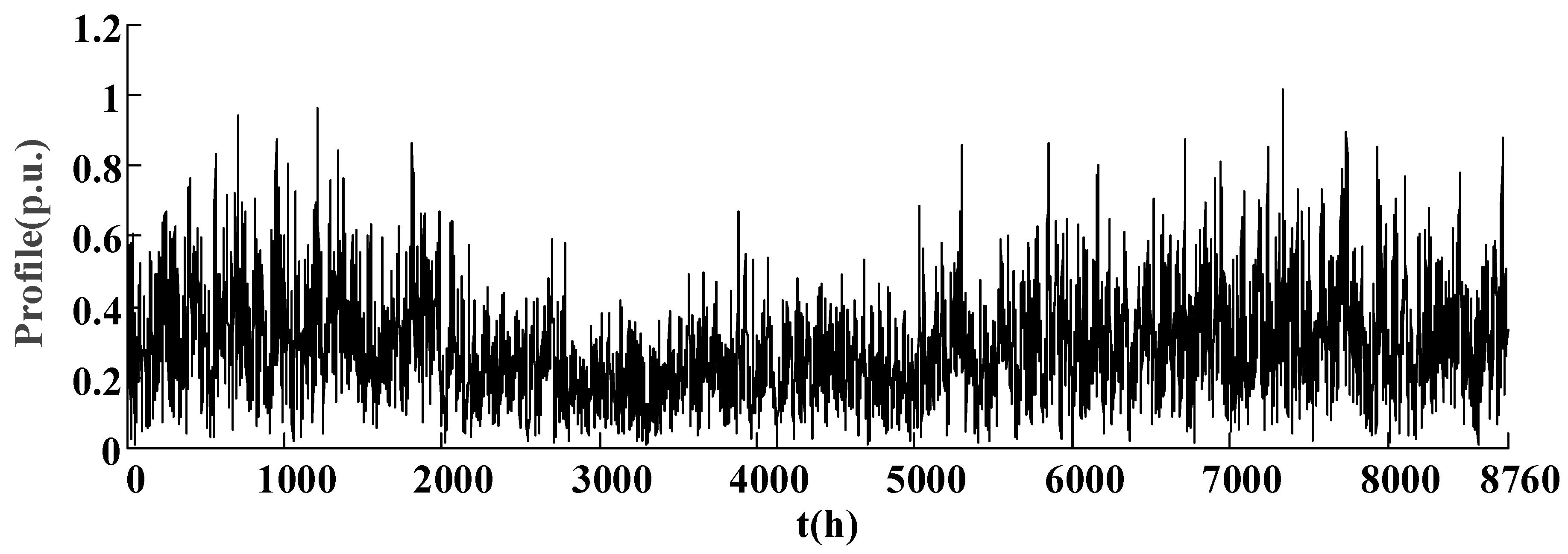
Assuming that the annual load curve, annual WT output curve and PV output curve in the distribution network are shown in Figure 2, Figure 3 and Figure 4, respectively. The typical scenarios for DES planning are generated by the clustering technique, containing the patterns of load demand, wind turbine output and photovoltaic output, which are shown in Figure A1 in the Appendix A. It is assumed that the maximum power and energy capacity of DES in planning are 1 MVA/4 MWh. The total number of nodes that DES can be installed with is up to 4.

The proposed model is implemented with the General Algebraic Modeling System (GAMS) optimization software and is solved by the commercial solver GUROBI [35]. GUROBI is an optimization package which has been widely applied in solving the MISOCP problem. The calculation is carried out on a PC with Intel Core i5 3.20 GHz CPU and 4 GB RAM.

5.1. Planning Results

5.1.1. Economic Benefits Improvement of ADN

The planning results are shown in

Table 4. Planning results of economic benefits improvement in IEEE 33-node system.

Type	Location	Power Capacity (kVA)	Energy Capacity (kWh)
Only lead-acid battery	14	120	610
	17	100	450
	30	390	1750
	32	210	930
Only Li-ion battery	17	120	990
	30	160	1420
	31	80	690
	33	100	900
Vanadium redox flow battery (VRB)	—	—	—

,

Table 5. Coordinated planning results of economic benefits improvement in IEEE 33-node system.

Type	Location	Power Capacity (kVA)	Energy Capacity (kWh)
Lead-acid battery	14	50	550
	17	70	810
	31	20	260
	32	60	690
Li-ion battery	31	130	1040
	32	80	650
VRB	—	—	—
Total	14, 17, 31, 32	410	4000

and

Table 6. Annual costs of DES planning in IEEE 33-node system.

Parameter	Operation Cost of ADN ($)	Investment Cost of DES ($)	${\mathit{C}}_{\mathbf{1}}\mathbf{(}\mathbf{\$}\mathbf{)}$
Without DES	1,303,663	—	1,303,663
Only lead-acid battery allocated	1,253,521	45,846	1,299,367
Only Li-ion battery allocated	1,226,924	71,172	1,298,096
Coordinated planning	1,235,782	57,503	1,293,285

. It can be seen that different types of DES have different performances. A lead-acid battery and Li-ion battery are both helpful but with different economic benefits in this case; a VRB is not selected to install because of the negative profit. In coordinated planning, the lead-acid battery and Li-ion battery are selected to allocate at the nodes 31 and 32 simultaneously. From Table 6, when only the Li-ion battery is allocated, the operation cost of ADN is lowest. However, the annual comprehensive cost is lowest in the coordinated planning, reducing by $10,378; the annual operation cost of the ADN is reduced by $67,881, a decrease of 5.21%. The price of lead-acid batteries is relatively low, but the cycle efficiency and the life cycle of the Li-ion battery are high. The two DESs have complementary advantages, and the economics of system operation is improved by coordinated planning. Although VRB has the highest cycle life compared to the other two DESs, VRB energy storage is expensive and has not been selected to be allocated in ADNs.

5.1.2. Power Fluctuation Smoothing

The planning results are shown in

Table 7. Planning results of power fluctuation smooth in IEEE 33-node system.

Type	Location	Power Capacity (kVA)	Energy Capacity (kWh)
Only Li-ion battery	10	260	1380
	16	160	1240
	17	180	540
	33	400	840
Only VRB	10	290	1450
	16	200	1240
	17	160	490
	33	350	820
Only lead-acid battery	—	—	—

and

Table 8. Power smooth results of DES planning in IEEE 33-node system.

	Power Fluctuation Cost ($)	Investment Cost of DES ($)	${\mathit{C}}_{\mathbf{2}}\mathbf{(}\mathbf{\$}\mathbf{)}$
Without DES	73,191	—	73,191
Only Li-ion battery allocated	24,692	44,125	68,817
Only VRB allocated	23,289	31,200	54,489

. The coordinated planning results are the same as the planning of only VRB in Table 7. It can be seen that the power fluctuation cost is reduced by $49,902 when a VRB is allocated, a decrease of 68.18%. Considering the investment cost of DES, $C_2$ is reduced by $18,702, a decrease of 25.43%.

In this case, because of the rapid power fluctuation of renewable DGs, DES needs to charge and discharge frequently to meet the demand for power smoothing. VRB has an exceptionally long lifetime compared with the other two DES types, making it is quite suitable for charging/discharging with high frequency. Although a lead-acid battery has an advantage in investment cost, it is not selected to install owing to its low life cycle.

With the development of DES technology, capital cost will be further reduced, and the economic benefits of DES will become more promising. In addition, DES can also perform the auxiliary service functions such as peak shaving, frequency support, and voltage regulation. Considering the above economic and environmental benefits, the practical value of DES will be further improved.

5.2. Evaluation of DES Planning

5.2.1. Economic Evaluation

The rate of return is set as the economic evaluation index, considering the benefit from reducing annual operation cost of ADN and the investment cost of DES, which is expressed as follows:

$$RR=\frac{B-C^{\mathrm{INV}}}{C^{\mathrm{INV}}}\times 100\%$$

(41)

where $B$ is the benefit from reducing the operation cost of ADN, which are formulated as follows:

$$B=C^{\mathrm{OPE},\mathrm{BEF}}-C^{\mathrm{OPE},\mathrm{AFT}}$$

(42)

where $C^{\mathrm{OPE},\mathrm{BEF}}$ is the operation cost of ADN before DES installed, and $C^{\mathrm{OPE},\mathrm{AFT}}$ is the operation cost after DES installed.

The results of the economic evaluation are shown in

Table 9. Results of the economic evaluation in IEEE 33-node system.

Parameter	Lead-Acid Battery	Li-Ion Battery	VRB	Coordinated Planning
$RR$	9.37	8.70	0	18.05

. The results show that a lead-acid battery has better economic benefits than a Li-ion battery. As VRB is not allocated owing to its high investment cost, it has no economic improvement. Furthermore, compared to the planning of single-type DES, the coordinated planning of DES significantly improves the economic benefits of ADNs.

5.2.2. Power Smoothing Evaluation

In the case of power fluctuation smooth, the power fluctuation coefficient is chosen as the evaluation index, which is the ratio of the power after DES smooth to original power output. The power fluctuation coefficient is expressed as:

$$f^{\mathrm{FLU}}=\frac{{{\displaystyle \sum }}_{s\in {\mathsf{\Omega }}_{\mathrm{S}}}\left\{{{\displaystyle \sum }}_{m\in {\mathsf{\Omega }}_{\mathrm{type}}}{{\displaystyle \sum }}_{i\in N_{\mathrm{N}}}{{\displaystyle \sum }}_{t\in N_{\mathrm{T}}}\left[\left(P_{s,t,i}^{\mathrm{DG}}+P_{s,t,i,m}^{\mathrm{DES}}\right)-\left(P_{s,t-1,i}^{\mathrm{DG}}+P_{s,t-1,i,m}^{\mathrm{DES}}\right)\right]\right\}{p}_s}{{{\displaystyle \sum }}_{s\in {\mathsf{\Omega }}_{\mathrm{S}}}\left\{{{\displaystyle \sum }}_{m\in {\mathsf{\Omega }}_{\mathrm{type}}}{{\displaystyle \sum }}_{i\in N_{\mathrm{N}}}{{\displaystyle \sum }}_{t\in N_{\mathrm{T}}}\left[P_{s,t,i}^{\mathrm{DG}}+P_{s,t-1,i}^{\mathrm{DG}}\right]\right\}{p}_s}$$

(43)

The evaluation results of power fluctuation smooth in Section 5.1.2 are shown in

Table 10. Power smoothing evaluation results in IEEE 33-node system.

Parameter	Lead-Acid Battery	Li-Ion Battery	VRB
$f^{\mathrm{FLU}}$	1.00	0.13	0.11

. The results show that VRB is more capable in power smooth of DG than Li-ion battery. As lead-acid battery is not allocated owing to its low cycle life, it has no ability for DG power smoothing.

5.3. Scalability Verification

The modified IEEE 123-node system is tested to verify the scalability of the proposed method on large-scale ADNs. The detailed parameters can refer to [36]. Three WTs and six PVs are integrated into the networks, of which the basic installation parameters are shown in

Table 11. Parameters of DGs.

Parameter	Wind Turbines			Photovoltaic Generators
Location	28	92	108	33	42	86	97	111	116
Capacity (kVA)	800	1200	1000	300	300	200	200	400	600

. The test case is shown in Figure 5.

The results of the economic benefits case study are shown in

Table 12. Planning results of economic benefits improvement in IEEE 123-node system.

Type	Location	Power Capacity (kVA)	Energy Capacity (kWh)
Only lead-acid battery	32	70	300
	47	110	1220
	58	80	760
	119	150	1720
Only Li-ion battery	—	—	—
Only VRB	—	—	—

and

Table 13. Annual costs of DES planning in IEEE 123-node system.

	Operation Cost of ADN ($)	Investment Cost of DES ($)	${\mathit{C}}_{\mathbf{1}}\mathbf{(}\mathbf{\$}\mathbf{)}$
Without DES	2,087,863	—	2,087,863
Only lead-acid battery allocated	2,032,369	45,846	2,078,215

. It can be seen from the results that a lead-acid battery is selected to allocate in ADN and the economic benefits are improved remarkably.

The results of the power fluctuation smooth by each DES type are shown in

Table 14. Planning results of power fluctuation smoothing in IEEE 123-node system.

Type	Location	Power Capacity (kVA)	Energy Capacity (kWh)
Only Li-ion battery	92	350	1350
	108	310	1280
	111	150	630
	116	190	740
Only VRB	92	380	1390
	108	330	1320
	111	120	610
	116	170	680
Only lead-acid battery	—	—	—

and

Table 15. Power smoothing results of DES planning in IEEE 33-node system.

	Power Fluctuation Cost ($)	Investment Cost of DES ($)	${\mathit{C}}_{\mathbf{2}}\mathbf{(}\mathbf{\$}\mathbf{)}$
Without DES	117,620	—	117,620
Only Li-ion battery allocated	69,443	44,125	113,568
Only VRB allocated	59,125	31,200	90,325

. The coordinated planning results are the same as the planning of VRB in Table 14. It can be seen from the results that the power fluctuation cost is reduced $58,495 by the integration of VRB, a decrease of 49.73%. The Li-ion battery is also applied to power smoothing, but the effect is inferior to VRB.

6. Conclusions

In this paper, a parameterized model for optimal DES planning in ADNs is presented. The typical scenarios for DES planning are generated by a clustering technique, containing the patterns of load demand, wind turbine output and photovoltaic output. To effectively solve the problem, the original MINLP model is transformed into a MISOCP model by convex conversion. The calculation and evaluation results show that through the presented method, the economic benefits of the distribution network have been significantly improved and the power fluctuation of DG has been smoothed through the optimal planning of DES.

With the rapid development of energy storage technology, it is foreseeable that the energy storage cost will be greatly reduced, and the applications of DES will become more and more extensive. The proposed method considers the economic and technical characteristics of DES and can achieve optimal planning with multiple types of DES in ADNs. It can provide reasonable schemes based on the parameterized model and support the distribution network planners to make decisions on the optimal sizing, allocation, and type selection of DES. It also shows great potential in real applications with different temporal and spatial scales, providing more effective support for renewable resource accommodation, voltage and frequency regulation, and self-healing control by detailed type selection and reasonable planning of DES.

References

- Wang, C.S.; Song, G.Y.; Li, P.; Ji, H.R.; Zhao, J.L.; Wu, J.Z. Optimal siting and sizing of soft open points in active electrical distribution networks. Appl. Energy 2017, 189, 301–309. [Google Scholar] [CrossRef]
- Rueda-Medina, A.C.; Padilha-Feltrin, A. Distributed Generators as Providers of Reactive Power Support—A Market Approach. IEEE Trans. Power Syst. 2013, 28, 490–502. [Google Scholar] [CrossRef]
- Sedghi, M.; Ahmadian, A.; Aliakbar-Golkar, M. Optimal storage planning in active distribution network considering uncertainty of wind power distributed generation. IEEE Trans. Power Syst. 2016, 31, 304–316. [Google Scholar] [CrossRef]
- Li, P.; Ji, H.R.; Wang, C.S.; Zhao, J.L.; Song, G.Y.; Ding, F.; Wu, J.Z. Coordinated Control Method of Voltage and Reactive Power for Active Distribution Networks Based on Soft Open Point. IEEE Trans. Sustain. Energy 2017, 8, 1430–1442. [Google Scholar] [CrossRef]
- Li, P.; Ji, H.R.; Wang, C.S.; Zhao, J.L.; Song, G.Y.; Ding, F.; Wu, J.Z. Optimal operation of soft open points in active distribution networks under three-phase unbalanced conditions. IEEE Trans. Smart. Grid 2019, 10, 380–391. [Google Scholar] [CrossRef]
- Li, C.; Liu, X.B.; Cao, Y.J.; Zhang, P.; Shi, H.Q.; Ren, L.Y.; Kuang, Y.H. A time-scale adaptive dispatch method for renewable energy power supply systems on islands. IEEE Trans. Smart. Grid 2016, 7, 1069–1078. [Google Scholar] [CrossRef]
- Saboori, H.; Hemmati, R.; Ghiasi, S.M.S.; Dehghan, S. Energy storage planning in electric power distribution networks–A state-of-the-art review. Renew. Sustain. Energy Rev. 2017, 79, 1108–1121. [Google Scholar] [CrossRef]
- Ji, H.R.; Wang, C.S.; Li, P.; Ding, F.; Wu, J.Z. Robust operation of soft open points in active distribution networks with high penetration of photovoltaic integration. IEEE Trans. Sustain. Energy 2019, 10, 280–289. [Google Scholar] [CrossRef]
- Shen, X.W.; Shahidehpour, M.; Han, Y.D.; Zhu, S.Z.; Zheng, J.H. Expansion Planning of Active Distribution Networks With Centralized and Distributed Energy Storage Systems. IEEE Trans. Sustain. Energy 2016, 8, 126–134. [Google Scholar] [CrossRef]
- Huang, S.J.; Wu, Q.W.; Oren, S.S.; Li, R.Y.; Liu, Z.X. Distribution locational marginal pricing through quadratic programming for congestion management in distribution networks. IEEE Trans. Power Syst. 2015, 30, 2170–2178. [Google Scholar] [CrossRef]
- Ji, H.R.; Wang, C.S.; Li, P.; Song, G.Y.; Yu, H.; Wu, J.Z. Quantified analysis method for operational flexibility of active distribution networks with high penetration of distributed generators. Appl. Energy 2019, 239, 706–714. [Google Scholar] [CrossRef]
- Poullikkas, A. A comparative overview of large-scale battery systems for electricity storage. Renew. Sustain. Energy Rev. 2013, 27, 778–788. [Google Scholar] [CrossRef]
- Chen, Q.X.; Zhao, X.Y.; Gan, D.H. Active-reactive scheduling of active distribution system considering interactive load and battery storage. Proc. CSEE 2017, 2, 29. [Google Scholar] [CrossRef]
- Lin, W.; Jin, X.D.; Mu, Y.F.; Jia, H.J.; Xu, X.D.; Yu, X.D.; Zhang, B. A two-stage multi-objective scheduling method for integrated community energy system. Appl. Energy 2018, 216, 428–441. [Google Scholar] [CrossRef]
- Hung, D.Q.; Mithulananthan, N.; Bansal, R.C. Integration of PV and BES units in commercial distribution systems considering energy loss and voltage stability. Appl. Energy 2014, 113, 1162–1170. [Google Scholar] [CrossRef]
- Wan, C.; Zhao, J.; Song, Y.H.; Xu, Z.; Lin, J.; Hu, Z.C. Photovoltaic and solar power forecasting for smart grid energy management. CSEE J. Power Energy Syst. 2016, 1, 38–46. [Google Scholar] [CrossRef]
- Dong, X.H.; Mu, Y.F.; Xu, X.D.; Jia, H.J.; Wu, J.Z.; Yu, X.D.; Yan, Q. A charging pricing strategy of electric vehicle fast charging stations for the voltage control of electricity distribution networks. Appl. Energy 2018, 225, 857–868. [Google Scholar] [CrossRef]
- Aneke, M.; Wang, M.H. Energy storage technologies and real life applications – A state of the art review. Appl. Energy 2016, 179, 350–377. [Google Scholar] [CrossRef]
- Carpinelli, G.; Celli, G.; Mocci, S.; Mottola, M.; Pilo, F.; Proto, D. Optimal integration of distributed energy storage devices in smart grids. IEEE Trans. Smart. Grid 2013, 4, 985–995. [Google Scholar] [CrossRef]
- Nick, M.; Cherkaoui, R.; Paolone, M. Optimal allocation of dispersed energy storage systems in active distribution networks for energy balance and grid support. IEEE Trans. Power Syst. 2014, 29, 2300–2310. [Google Scholar] [CrossRef]
- Xiao, J.; Zhang, Z.Q.; Bai, L.Q. Determination of the optimal installation site and capacity of battery energy storage system in distribution network integrated with distributed generation. IET Gener. Trans. Distrib. 2016, 10, 601–607. [Google Scholar] [CrossRef]
- Bai, L.Q.; Jiang, T.; Li, F.X.; Chen, H.H.; Li, X. Distributed energy storage planning in soft open point based active distribution networks incorporating network reconfiguration and DG reactive power capability. Appl. Energy 2018, 210, 1082–1091. [Google Scholar] [CrossRef]
- Nick, M.; Cherkaoui, R.; Paolone, M. Optimal planning of distributed energy storage systems in active distribution networks embedding grid reconfiguration. IEEE Trans. Power Syst. 2018, 33, 1577–1590. [Google Scholar] [CrossRef]
- Liu, Y.K.; Zhang, L.; Tao, F.; Wang, L. Resource service sharing in cloud manufacturing based on the Gale–Shapley algorithm: Advantages and challenge. Int. J. Comput. Integr. Manuf. 2017, 30, 420–432. [Google Scholar] [CrossRef]
- Argoneto, P.; Renna, P. Supporting capacity sharing in the cloud manufacturing environment based on game theory and fuzzy logic. Enterp. Inf. Syst. 2016, 10, 193–210. [Google Scholar] [CrossRef]
- Zidar, M.; Georgilakis, P.S.; Hatziargyriou, N.D.; Capuder, T.; Škrlec, D. Review of energy storage allocation in power distribution networks: applications, methods and future research. IET Gener. Trans. Distrib. 2015, 10, 645–652. [Google Scholar] [CrossRef]
- Luo, X.; Wang, J.H.; Dooner, M.; Clarke, J. Overview of current development in electrical energy storage technologies and the application potential in power system operation. Appl. Energy 2015, 137, 511–536. [Google Scholar] [CrossRef] [Green Version]
- Wang, C.S.; Jiao, B.Q.; Guo, L.; Yuan, K.; Sun, B. Optimal planning of stand-alone microgrids incorporating reliability. J. Modern Power Syst. Clean Energy 2014, 2, 195–205. [Google Scholar] [CrossRef] [Green Version]
- Kanungo, T.; Mount, D.M.; Netanyahu, N.S.; Piatko, C.D.; Silverman, R.; Wu, A.Y. An efficient k-means clustering algorithm: analysis and implementation. IEEE Trans. Pattern Anal. Mach. Intell. 2002, 24, 881–892. [Google Scholar] [CrossRef]
- Wang, S.X.; Wang, K.; Teng, F.; Strbac, G.; Wu, L. An affine arithmetic-based multi-objective optimization method for energy storage systems operating in active distribution networks with uncertainties. Appl. Energy 2018, 223, 215–228. [Google Scholar] [CrossRef]
- Sauer, D.U.; Wenzl, H. Comparison of different approaches for lifetime prediction of electrochemical systems—Using lead-acid batteries as example. J. Power Sour. 2008, 176, 534–546. [Google Scholar] [CrossRef]
- Boyd, S.; Vandenberghe, L. Convex Optimization; Cambridge University Press: Cambridge, UK, 2004. [Google Scholar]
- Farivar, M.; Low, S.H. Branch flow model: Relaxations and convexification (Part I). IEEE Trans. Power Syst. 2013, 28, 2554–2564. [Google Scholar] [CrossRef]
- Baran, M.E.; Wu, F.F. Network reconfiguration in distribution systems for loss reduction and load balancing. IEEE Trans. Power Del. 1989, 4, 1401–1407. [Google Scholar] [CrossRef]
- Brook, A.; Kendrick, D.; Meeraus, A. GAMS, a user’s guide. ACM Signum Newsl. 1988, 23, 10–11. [Google Scholar] [CrossRef]
- Chen, X.; Wu, W.C.; Zhang, B.M. Robust restoration method for active distribution networks. IEEE Trans. Power Syst. 2016, 31, 4005–4015. [Google Scholar] [CrossRef]
Figure 1.
Structure of the modified IEEE 33-node system.
Figure 2.
Annual load curve.
Figure 3.
Annual power output of wind turbines (WTs).
Figure 4.
Annual power output of photovoltaic generators (PVs).
Figure 5.
Structure of the modified IEEE 123-node system.