A New Model for Constant Fuel Utilization and Constant Fuel Flow in Fuel Cells

Department of Mathematics and Computer Science, University of Missouri, St. Louis, MO 63121, USA
Appl. Sci. 2019, 9(6), 1066; https://doi.org/10.3390/app9061066
Submission received: 11 December 2018
/
Revised: 28 February 2019
/
Accepted: 6 March 2019
/
Published: 14 March 2019
(This article belongs to the Special Issue Progress in Solid-Oxide Fuel Cell Technology)
Abstract
:This paper presents a new model of fuel cells for two different modes of operation: constant fuel utilization control (constant stoichiometry condition) and constant fuel flow control (constant flow rate condition). The model solves the long-standing problem of mixing reversible and irreversible potentials (equilibrium and non-equilibrium states) in the Nernst voltage expression. Specifically, a Nernstian gain term is introduced for the constant fuel utilization condition, and it is shown that the Nernstian gain is an irreversibility in the computation of the output voltage of the fuel cell. A Nernstian loss term accounts for an irreversibility for the constant fuel flow operation. Simulation results are presented. The model has been validated against experimental data from the literature.
1. Introduction
Fuel cells [1,2,3,4] convert chemical energy into electrical energy and are fast emerging as one of the major alternatives to fossil-fuel-based sources of energy. Modeling is often an integral part of fuel cell research, spanning areas from new material investigation [5] to system integration [6] to control of the plant [7]. Even though many models of fuel cells and fuel cell systems have already been proposed in the literature, new models continue to be developed, improving upon the state of the art. This paper presents an improved fuel cell model for two operating conditions: constant fuel utilization and constant fuel flow (with the constant fuel flow operation being analyzed in the context of two different modes for the oxidant—the constant oxygen flow mode and the constant oxygen stoichiometry mode). The need for a new model arose because of a recently identified problem [8] in a family of commonly used models in the literature. The problem involves the (erroneous) mixing of reversible and irreversible potentials in the computation of the cell output voltage. The present paper seeks to solve the problem by separating the irreversibilities from the reversible (equilibrium) potential of the fuel cell. The solution is achieved by introducing a novel “Nernstian gain” term and establishing it as an irreversibility for the constant fuel utilization condition. A Nernstian loss term, somewhat akin in spirit to traditional fuel cell losses, is used to analyze the constant fuel flow operation.
The remainder of this paper is organized as follows. A brief survey of previous work on fuel cell modeling is presented in Section 2. Section 3 describes the problem. Section 4 develops a model for the constant fuel utilization mode of operation of the cell. The constant fuel flow mode is modeled in Section 5. Conclusions are drawn in Section 6.
2. A Brief Review of the Literature
Typical classifications of fuel cells are based on the type of electrolyte used in the cell, the operating temperature range, the fuel used, and other factors [9,10]:
- Direct methanol fuel cell (DFMC), about 60 C
- Proton exchange membrane (or polymer electrolyte membrane) fuel cell (PEMFC), less than 120 C, typically about 80 C
- Alkaline fuel cell (AFC), about 100 C or less
- Phosphoric acid fuel cell (PAFC), about 150–200 C
- Molten carbonate fuel cell (MCFC), about 600–700 C
- Solid oxide fuel cell (SOFC), about 600–1000 C
Reversible fuel cells [11] represent another class of fuel cells that, in addition to producing electricity from hydrogen and oxygen, can use electricity to produce, by electrolysis, hydrogen and oxygen from water. Microbial fuel cells [12] are yet another category of fuel cells where biological organisms (bacteria, for example) act as the electrocatalyst.
The literature on the modeling of fuel cells is expansive (see, for example, [9,13,14,15,16,17,18,19,20,21]). The fuel cell is a complex, non-linear system, and not all aspects of the physics, chemistry and engineering of the system are completely understood yet. Given the enormity of the problem, a single model typically focuses on one particular aspect (e.g., liquid water removal from a PEMFC [22] or real-time simulation [23]) of the system.
Fuel cell models are usually characterized by the number of physical dimensions (number of different geometrical axes) they consider. Clearly, this number can vary from zero to three. Zero-dimensional (0-D) models (e.g., [24,25,26]) employ a concentrated (as opposed to distributed) or lumped representation of the parameters or metrics (e.g., voltage, current, temperature or species partial pressures) under consideration and therefore make more use of mathematical abstraction than the spatial geometry of the cell. In other words, the variation of parameters along/within the cell is ignored, that is, the “local” and “global” values are the same in such models. This type of modeling is particularly useful when the interaction of the cell with other components of the (integrated) system is to be investigated (e.g., the modeling of SOFC-based hybrid power generation systems) [27]. A simple, lumped, dynamic model of an integrated SOFC plant is developed for power system simulation in [28], building upon which a large number of fuel cell models have been proposed in the literature (see, e.g., [6,7,29,30,31,32,33,34,35,36,37,38,39,40,41,42,43,44,45,46,47,48,49,50,51,52,53,54,55]).
One-dimensional (1-D) models (e.g., [23,34,35,56,57]) take into account the variation of the relevant metrics (electrochemical, physical, or thermal) along only one dimension of the cell, ignoring the other two dimensions. For instance, a 1-D model can compute local changes in current density in axial directions of tubular fuel cells [58]. Zero- and one-dimensional models are often quite effective for control purposes.
Two-dimensional (2-D) models (e.g., [59,60,61]) consider a two-dimensional cross-section of the cell geometry, ignoring the variations along the third dimension.
Three-dimensional (3-D) models (e.g., [62,63,64,65,66,67]) use distributed (not lumped) metrics or parameters and are the closest to the physical geometry of the cell, describing spatial properties in each of the three coordinates. Because of their high computational costs, 3-D models are somewhat more esoteric than 2-D or 1-D models; in Reference [68], we find an example of the reduction of a 3-D model to 2-D without significant compromises with the quality of results.
Zero-dimensional or lumped models are also referred to as macro-models [27]. Because models in two or three dimensions look at finer levels of granularity, they are sometimes called micro-models [69]. Length-scales and time-scales are important issues in the modeling of fuel cells; for a review of multi-scale modeling of SOFCs from quantum (sub-atomic) to atomistic to continuum, see Reference [70].
On top of the dimensional categories, fuel cell models can also be broadly classified as:
- mechanistic (theoretical)
- empirical (experimental)
- semi-empirical
- data-driven (machine-learning-based)
Mechanistic models are obtained (derived) theoretically, using theories from, e.g., electrochemistry, thermodynamics, fluid dynamics and engineering; well-known examples include the use of fundamental, phenomenological equations such as the Butler–Volmer equation for voltage, the Stefan–Maxwell equation for diffusion, and the Nernst–Plank equation for species transport [71,72].
Empirical models (e.g., [73,74]), on the other hand, use data obtained from actual experiments on physical fuel cells to propose relationships among the variables of interest, especially relationships that would otherwise be difficult to arrive at from theory alone.
Semi-empirical models (e.g., [61,75]) employ a mix of theory and experimentation. The line between the theoretical and the semi-empirical is sometimes blurred.
Data-driven (or data-oriented) models are a relatively recent development in the field. This approach is capable of creating predictive models for fuel cells and fuel cell systems by using statistical and algorithmic analysis of experimental (or simulated) data. Data-driven models, sometimes referred to as “black-box” models, employ techniques from the machine learning [76] or artificial intelligence [77] paradigm. Examples of data-driven models include Reference [38], where genetic programming [78] is used in a supervised learning setting for static and dynamic (load-following) modeling of SOFCs, and Reference [79] where differential evolution [80] is used to optimize seven parameters for modeling the polarization curve of a PEMFC stack. Given the rather loose connection between theoretical (mechanistic) principles and the data-driven approach, it can be argued that data-driven models verge on the empirical or the semi-empirical.
3. The Problem
The Nernst equation, which is the cornerstone of fuel cell thermodynamics, provides an expression for the reversible thermodynamic potential, also known as the equilibrium voltage or the open-circuit electromotive force (EMF), of the fuel cell [1]:
where is the reference (standard) EMF at unit activity and atmospheric pressure, i and j are the numbers of reactant and product species, a represents the activity, is the stoichiometric coefficient of species i, R is the universal gas constant, F is Faraday’s constant, n is the number of electrons transferred for each molecule of the fuel participating in the reaction, and T is the temperature. For a hydrogen–oxygen fuel cell (e.g., solid oxide fuel cell (SOFC) or proton exchange membrane fuel cell (PEMFC)), hydrogen and oxygen are the reactants, and the product is water (or steam). The reference EMF, , depends on temperature T:
where is the standard EMF at temperature , and is the change in entropy. The activity a of an ideal gas is expressed in terms of its pressure (or partial pressure) p:
where is the standard-state pressure (1 atm). At high temperatures, such as 1000 C (as in solid oxide fuel cells), steam can be assumed to behave as an ideal gas, and therefore
Using = 1 atm, and noting that for a hydrogen fuel cell, we have the following version of the Nernst equation for solid oxide fuel cells:
If the fuel cell is operated below 100 C, so that liquid water is produced (as in proton exchange membrane fuel cells), the activity of water can be taken to be unity ( = 1). In that case, the Nernst equation takes the form
The terminal (load) voltage is generally obtained by subtracting from the following types of losses (or “irreversibilities”):
- activation loss
- concentration loss
- ohmic loss
- losses due to fuel crossover and internal current.
The practice of expressing—either directly or indirectly via the partial pressures—the Nernst EMF as a function of cell current is rather common in the literature (e.g., [33,34]). Building upon References [28,29], a major piece of work [7] on control strategies for SOFC operation developed a model for the constant fuel utilization condition using the following form of the Nernst equation:
where , , and are valve molar constants [28], [28,38,39], is the ratio of hydrogen to oxygen input molar flow rates [7], u is the fuel utilization ratio [7,28], and is the load current. This model, or one of its variants, has been used in many papers in the fuel cell literature (e.g., [6,38]). (A detailed re-derivation of Equation (8) can be found in, for example, Reference [8].) Of the four types of losses mentioned above, the models in References [7,28] consider only the ohmic loss and obtain the output (load) voltage, V, as
where is given by Equation (8), and r is the ohmic resistance of the cell.
As explained in Reference [8], the problem with Equation (8) is that it mixes equilibrium and non-equilibrium expressions. The Nernst voltage (EMF) is the reversible thermodynamic potential that applies only to the equilibrium condition of the cell; the equilibrium is lost when current is drawn from the cell. In other words, the Nernst voltage is by definition the open-circuit EMF and cannot therefore be expressed in terms of the load current [8].
To alleviate the aforementioned problem presented by Equation (8), we present an improved model in the following two sections.
All fuel cell models in the literature make simplifying assumptions and approximations; the present model also makes the standard set of assumptions that includes the following:
- The gases used in the chemical reactions are ideal and uniformly distributed.
- The fuel cell is considered a single “lumped” system; the species enter the cell through one end and exit through the other end.
- The only reaction that contributes to voltage takes place between hydrogen and oxygen. There is no parasitic reaction.
- All reactants generate their ideal number of electrons.
- No fuel or oxidant crosses the electrolyte.
- The gases have a uniform concentration in the supply channels; there are no pressure losses.
- The flows are incompressible.
- The fuel and oxidant are available as soon as they are needed (no delays).
- The partial pressures of the gases in the bulk of the anode and the cathode channels are assumed to be the same as those at the triple-phase-boundaries.
- The temperature is fixed (stable) at all times, and temperature variations across the cell are ignored.
- The operating voltage is uniform over the cell.
- Heat losses are negligible (the fuel cell is well insulated).
- There is no gas leakage.
- The Nernst equation can be applied.
4. Constant Fuel Utilization
Following Reference [7], the following two parameters are kept constant in this section: u (Equation (11)) and (Equation (17)). This corresponds to the operating condition known as constant fuel utilization ratio/factor condition or, equivalently, constant stoichiometry condition.
Hydrogen partial pressure is given by [28,38]
where is a valve molar constant [28], represents the input molar flow rate (mol/s) of hydrogen fuel, and is the hydrogen flow rate (mol/s) that takes part in the reaction.
Using the definition of fuel utilization ratio u,
we have
The ratio of two different hydrogen partial pressures is then given by
Since the reaction rate is given (from electrochemistry) by
the pressure ratio reduces to
Next, the partial pressure for oxygen is expressed as
where is a valve molar constant [28], denotes the oxygen input molar flow rate, and is the oxygen flow rate that reacts. Noting that is the ratio of hydrogen-to-oxygen input flow rates,
and that
we have
Now, by using the definition of u, we obtain
Two different oxygen partial pressures, then, have the following ratio:
Water (steam) partial pressure is expressed as
where is a valve molar constant [28], and is the flow rate of the water vapor (steam) that is produced in the reaction. The final and initial pressures are then related by
The change in the voltage corresponding to the changes in the pressures is given by
which, by Equations (15), (21) and (25), yields
The above expression for voltage change shows that, for an increase in the cell current, is positive, representing a gain. (Following the present approach, an expression for is derived in the next section for the constant fuel flow condition. For an increase in current, for the constant fuel flow case is negative, representing a loss.) Now, setting , and calling
where is a unit-free number, we can express the output voltage as follows:
where , determined from the initial cell conditions at open circuit, is given by Equation (6), > 1 (corresponding to an increase in current), and is small (ideally zero, corresponding to the open-circuit condition). A zero value of , however, will render undefined. Since “it must be borne in mind that the logarithmic model does not work at very low currents, especially at zero” [1], for practical purposes, we set = 1 A. This allows us to be “lazy” ([4], p. 50) and “simplify” ([1], p. 37) Equation (29) to
where in expressed in Amperes. (Mathematically, the argument of logarithm is dimensionless (unitless). The propriety of taking the logarithm of a dimensioned quantity has long been debated [81,82,83,84]. In the fuel cell literature, however, it seems standard practice to do so (see, for example, References [1,3,4,85]). A classic example of the logarithm of a dimensioned quantity is the famous Tafel equation [86], which expresses the activation loss as , where J stands for the current density.)
Equation (30) holds for A and > 1, and smoothes out, by approximation, the transition from = 0 to = 1 A.
The second term in Equation (30), which is positive for A, represents a “Nernstian” gain. This can be given a physical interpretation. The fact that both u and are constant implies a constant fuel (hydrogen) utilization ratio and a constant oxidant (oxygen) utilization ratio. This means that: (a) hydrogen and oxygen are replenished as soon as they are consumed in the fuel cell; and (b) as current increases, so do hydrogen and oxygen supplies, causing the reactant concentrations to go up, thereby producing a higher potential according to the Nernst equation. The product (water or steam) concentration also increases with current under the constant-u-and-constant- condition, but any decrease in potential brought about by the increase in the product concentration is more than offset by the increase in potential caused by the corresponding increase in the reactant concentrations. This Nernstian gain is irreversible, much the same way that the traditional concentration loss (or mass transport loss or Nernstian loss) is irreversible.
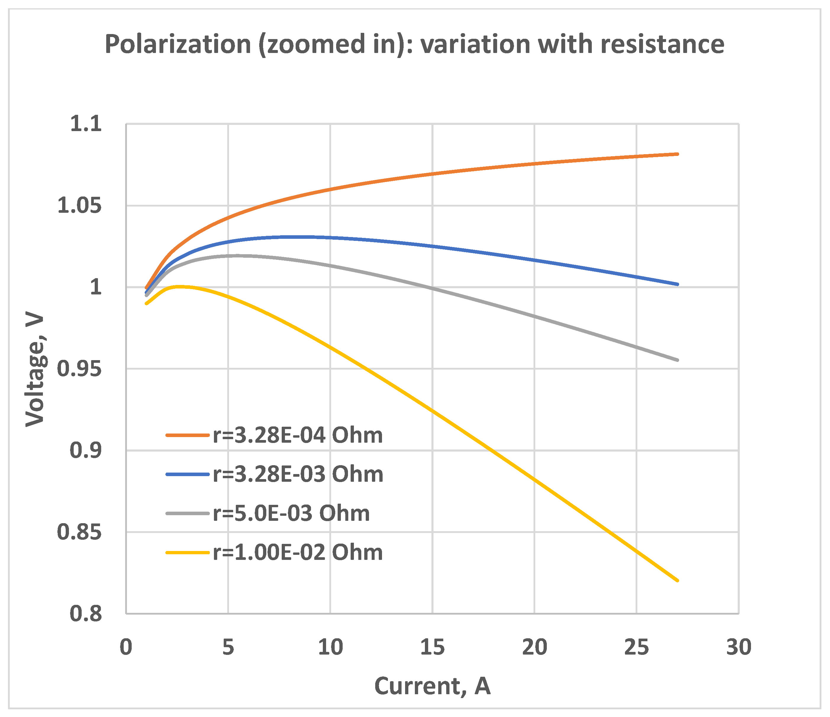
Figure 1 and Figure 2 present polarization curves for the constant fuel utilization condition using fuel cell parameters shown in Table 1. The data in Table 1 were taken from References [7,28]. , to be found from Equation (6) by plugging in the initial partial pressures and the , is taken to be 1 V in Figure 1 and Figure 2. Figure 1 shows the two irreversibilities—Nernstian gain and ohmic loss—separately. The magnitude of the ohmic loss is plotted, ignoring the sign. The Nernstian gain, being a logarithmic function, is monotone increasing. The shape of the output voltage curve is determined by how much of the Nernstian gain is offset by the ohmic loss for a given current. The effect of the Nernstian gain can be seen rather conspicuously in the hump in the output voltage at low currents. The output voltage equals the Nernst voltage at the point where
an equation that is difficult to solve analytically. Figure 2 shows, for low currents, how the polarization plot’s hump varies for different values of the cell resistance. (An r of 3.28125 × 10 is used in Figure 1.)
It can be argued that, in theory, in the constant hydrogen and oxygen utilization condition, the concentration loss (mass transport loss) is mitigated or almost eliminated. (Of course much depends on the physical characteristics of the reactant supply systems, reformer and control mechanisms, time-delays in the diffusion process between the channel and the three-phase-boundary, etc.) Under the assumption of the ideal conditions in our lumped model, the concentration loss is negligible or zero in Equation (30).
For the constant fuel utilization operation, Equations (11), (12), (20) and (23) show that , , and all are directly proportional to (i.e., increase linearly with) the input fuel flow rate. This is shown in Figure 3, where the straight lines have been obtained using the parameter values in Table 1. All three lines have a zero intercept, and their slopes are given by
The polarization characteristics produced by the constant fuel utilization model are similar in nature to those in the literature.
The constant fuel utilization model is validated with experimental data, taken from Reference [87], on a Siemens-Westinghouse high-power-density solid oxide fuel cell with ten channels (APS HPD10). The data were obtained graphically (as in References [88,89,90,91]) from the results of Test 1018 in Figures 9 and 10 of Reference [87]. Figure 4 presents a model-versus-experimental comparison. The average absolute relative error was found to be 3.74%, a figure that is generally considered in the literature to indicate good agreement between theory and practice. Since the experimental current reported in Figures 9 and 10 of Reference [87] starts at 87 A for Test 1018, the Nernst voltage was estimated, by an approximate extrapolation (as in Figure 7-17 of Reference [85]), to be 0.74 V. The temperature was 1273 K, and the cell area was 870 cm [87]. The resistance was estimated (following Reference [61]), from the slope of the (approximately) linear part of the experimental polarization (current-voltage) curve, to be 0.0006 . The slope was obtained from the equation of the straight line derived by a least-squares linear regression fit of all but the first five experimental data points.
Voltage transients (dynamics) due to hydrogen concentration changes are an important issue in fuel cell operation and are investigated in References [92,93], where the constant fuel utilization mode is used to implement a current-based fuel control strategy (changing the fuel flow rate in proportion to the cell current) to keep voltage transients under check. Constant fuel utilization is also shown to be beneficial for control purposes of SOFC systems in Reference [94], where it is reported that a suitably chosen constant fuel utilization operation leads to nearly maximum-efficiency performance for variable loads.
5. Constant Fuel Flow
This section considers a constant input fuel flow rate; that is, does not vary with . The two operating modes—constant fuel utilization (the preceding section) and constant fuel flow (the present section)—are summarized in Figure 5 where the line parallel to the current axis represents a constant input fuel flow rate. The line starting at the zero current point represents a constant fuel utilization ratio and has a slope of , a fact that is easily established from Equations (11) and (14). (Figure 5 uses data from Table 1.)
While the fuel flow rate is held constant, oxygen flow control can be done in one of two ways: either maintain a constant ratio of hydrogen-to-oxygen input flow rates or maintain a constant stoichiometric ratio for oxygen. We analyze these two modes in the following two subsections.
5.1. Constant Hydrogen-Oxygen Input Flow Ratio
This subsection treats the operating condition of (Equation (17)) being held constant. The constancy of both and means that the oxygen input molar flow rate, , is also constant.
The ratio of two different partial pressures, corresponding to two different current values, is obtained as
Two different oxygen partial pressures, corresponding to and , are then related by:
From Section 4, we know that the final and initial steam pressures have a ratio given by Equation (25).
The change in voltage corresponding to the changes in the three pressures is given by
which, by Equations (25), (33) and (36), becomes
The above expression shows that, for an increase in the cell current, is negative, representing a loss. As in Section 4, expressing all currents in units of Amperes, and setting = 1 A and in the above equation, we have
The output (load) voltage, V, for the constant fuel flow mode is then given by
where , the reversible (equilibrium) potential, is given by Equation (6), and the second term on the right side represents an irreversible loss (Nernstian loss). (Equation (40) holds for A.) This Nernstian loss is explained by the fact that, with and held constant (note that the constancy of both and implies that of , too), reactant concentrations decrease and product concentration increases with increasing current. Equation (32) shows that, for a fixed , hydrogen pressure decreases linearly with increasing current. Similar is the behavior of with respect to current, when the two input flow rates are kept fixed (see Equation (35)). The behavior of is opposite; as shown by Equation (24), grows linearly with current. Interestingly, given current, is (conditionally) independent of . Figure 6 shows an example of how the three pressures change with current when the flow rates are held constant (the plots are produced with the parameter values in Table 1 and a fixed = 0.1 mol/s).
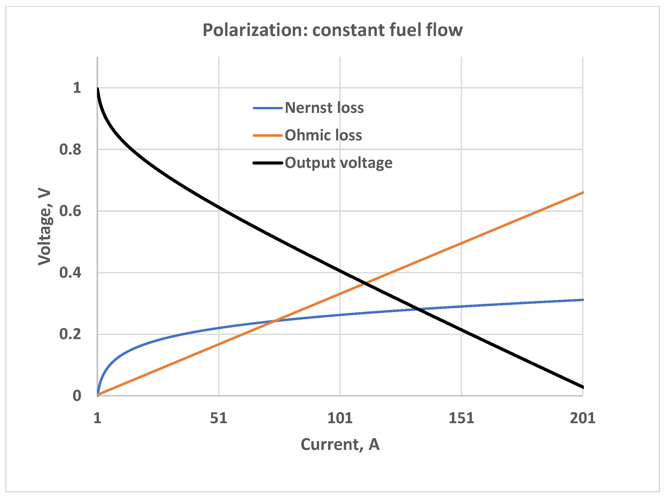
The polarization curve for the constant flow rate condition (see Equation (40)) is shown in Figure 7 where the Nernst loss and ohmic loss are shown separately. The positive magnitudes of the two losses are shown; their signs are accounted for in the output voltage calculation. This figure uses the parameter values in Table 1 along with = 1 V, = 0.004 mol/s and r = 3.28125 × 10. The polarization plot shows the same trend that is generally seen in constant flow polarization in the literature.
The effect of the (constant) input fuel flow rate on the polarization behavior is presented in Figure 8, where three different values are used: 0.02 mol/s, 0.004 mol/s, and 0.001 mol/s. The figure shows that a higher input flow rate leads to a higher voltage for the same load current, an observation that fits in with the concept of a higher reactant concentration leading to a higher potential. Figure 9 shows the variation in power characteristics corresponding to different (constant) fuel flow rates (the fuel flow rates in this figure are the same as the ones in Figure 8); a higher fuel flow rate results in higher power, as expected. Figure 8 and Figure 9 use = 1 V and r = 3.28125 × 10.
Results of model validation are shown in Figure 10, where the experimental polarization data (on a planar single SOFC at ENEA laboratories) were graphically obtained from Reference [61]. The results show reasonably good agreement, with an average absolute relative error of 3.96%. The validation was done under the following operational condition [61] for both the model and the experiment: temperature: 923 K; pressure: atmospheric; : 0.00112 mol/s; : 0.00038 mol/s; anode: 96% hydrogen, 4% water; cathode: 21% oxygen, 79% nitrogen; cell area: 121 cm. The calculated value of the model was 1.122 V, with the value of in Equation (2) estimated from the following relationship [61,95,96]:
Given the “systematic error of about 0.018 V” in Reference [61] between the theoretical Nernst voltage and its experimental counterpart, the experimental in the present validation was taken as 1.122 V − 0.018 V = 1.104 V. A resistance of 0.0043 was used for validation; this value was obtained as the approximate slope of the (nearly) linear part of experimental polarization plot, as computed from a least-squares linear fit to the experimental data points (excluding the first four points).
5.2. Constant Oxygen Stoichiometry Ratio
We consider a stoichiometric ratio, S, for oxygen:
where S is held constant (unlike Section 5.1 where is kept constant). The fuel flow rate is kept constant, as before.
Using the stoichiometric ratio, we can express oxygen partial pressure as:
Two different oxygen partial pressures have the following ratio:
The above equation shows that for , the change in voltage is negative, implying a loss. As before, expressing currents in Amperes and setting = 1 A and , we have for A the following expression for the output voltage:
where is given by Equation (6).
The polarization plot for the constant oxygen stoichiometry (and constant fuel flow) condition is shown in Figure 11 where the Nernstian loss is plotted separately (the Nernstian loss is plotted as a negative value). The polarization curve shows characteristics similar to those in the literature: after the initial drop, the voltage shows an approximately linear decay for much of the operating range before dropping heavily at high currents. In Figure 11, = 0.0009 mol/s. Figure 12 shows the effect of the (constant) fuel flow rate on the polarization performance. Power-versus-current behavior for the constant-fuel-flow-constant-oxygen-stoichiometry condition is presented in Figure 13. Figure 11, Figure 12 and Figure 13 use the relevant data from Table 1 and = 1 V. Figure 12 and Figure 13 use the following values: 0.004 mol/s, 0.002 mol/s, and 0.0009 mol/s.
6. Conclusions
An improved fuel cell model for constant fuel utilization control and constant fuel flow control was developed in this paper. By deriving expressions for two irreversibilities—a Nernstian gain (for the constant fuel utilization mode) and a Nernstian loss (for the constant fuel flow mode)—the model solves the problem of mixing up of reversible and irreversible potentials in the Nernst EMF expression. To our knowledge, the concept of the Nernstian gain and the characterization of the Nernstian gain as an irreversibility has not yet been presented in the fuel cell literature. The model thus eliminates the (flawed) need in previously published models for the open-circuit Nernst voltage to be expressed as a function of the load current. The model was validated against experimental data from the literature, with the average absolute relative error being less than 4%.
Funding
This research was funded in part by United States National Science Foundation Grant IIS-1115352.
Acknowledgments
Conflicts of Interest
The author declares no conflict of interest.
Abbreviations
The following abbreviations are used in this manuscript:
| SOFC | Solid oxide fuel cell |
| PEMFC | Proton exchange membrane fuel cell |
| EMF | Electromotive force |
| Nomenclature | |
| Nernst potential (open-circuit EMF) of a single cell, V | |
| Standard (reference) EMF of a single cell, V | |
| Standard (reference) EMF of a single cell at temperature , V | |
| V | Output terminal voltage of a single cell, V |
| T | Temperature, K |
| n | Number of electrons transferred |
| a | Activity |
| Activity of hydrogen | |
| Activity of oxygen | |
| Activity of water vapor (steam) | |
| Change in entropy, J/(mol K) | |
| p | Pressure or partial pressure, atm |
| Standard-state pressure, atm | |
| Partial pressure of hydrogen, atm | |
| Partial pressure of oxygen, atm | |
| Partial pressure of water vapor, atm | |
| Fuel cell current, A | |
| u | Fuel utilization ratio |
| Ratio of hydrogen-to-oxygen input flow rates | |
| Valve molar constant for hydrogen, mol/(s atm) | |
| Valve molar constant for oxygen, mol/(s atm) | |
| Valve molar constant for water vapor, mol/(s atm) | |
| Modeling constant, mol/(s A) | |
| Hydrogen input flow rate, mol/s | |
| Hydrogen output flow rate, mol/s | |
| Hydrogen flow rate that takes part in the reaction, mol/s | |
| Oxygen input flow rate, mol/s | |
| Oxygen output flow rate, mol/s | |
| Oxygen reacting flow rate, mol/s | |
| Water vapor output flow rate, mol/s | |
| Water vapor flow rate produced in the reaction, mol/s | |
| r | Ohmic resistance of a single cell, Ohm |
| R | Universal gas constant, J/(mol K) |
| F | Faraday’s constant, Coulombs/mol |
References
- Larminie, J.; Dicks, A. Fuel Cell Systems Explained, 2nd ed.; Wiley: Chichester, UK, 2003. [Google Scholar]
- Singhal, S.C.; Kendall, K. (Eds.) High-Temperature Solid Oxide Fuel Cells: Fundamentals, Design and Applications; Elsevier: Amsterdam, The Netherlands, 2003. [Google Scholar]
- Barbir, F. PEM Fuel Cells: Theory and Practice, 2nd ed.; Elsevier: Amsterdam, The Netherlands, 2013. [Google Scholar]
- O’Hayre, R.; Cha, S.W.; Colella, W.; Prinz, F.B. Fuel Cell Fundamentals, 3rd ed.; John Wiley: Hoboken, NJ, USA, 2016. [Google Scholar]
- Cavallaro, A.; Pramana, S.S.; Ruiz-Trejo, E.; Sherrell, P.C.; Ware, E.; Kilner, J.A.; Skinner, S.J. Amorphous- cathode-route towards low temperature SOFC. Sustain. Energy Fuels 2018, 2, 862–875. [Google Scholar] [CrossRef]
- Radisavljevic, V. On controllability and system constraints of the linear models of proton exchange membrane and solid oxide fuel cells. J. Power Sources 2011, 196, 8549–8552. [Google Scholar] [CrossRef]
- Li, Y.H.; Choi, S.S.; Rajakaruna, S. An analysis of the control and operation of a solid oxide fuel-cell power plant in an isolated system. IEEE Trans. Energy Convers. 2005, 20, 381–387. [Google Scholar] [CrossRef]
- Chakraborty, U.K. Reversible and irreversible potentials and an inaccuracy in popular models in the fuel cell literature. Energies 2018, 11, 1851. [Google Scholar] [CrossRef]
- Kakac, S.; Pramuanjaroenkij, A.; Zhou, X.Y. A review of numerical modeling of solid oxide fuel cells. Int. J. Hydrogen Energy 2007, 32, 761–786. [Google Scholar] [CrossRef]
- Comparison of Fuel Cell Technologies, Fuel Cell Technologies Office, U.S. Department of Energy. Available online: https://www.energy.gov/eere/fuelcells/comparison-fuel-cell-technologies (accessed on 16 February 2019).
- Ito, H.; Miyazaki, N.; Ishida, M.; Nakano, A. Efficiency of unitized reversible fuel cell systems. In. J. Hydrogen Energy 2016, 41, 5803–5815. [Google Scholar] [CrossRef]
- Santoro, C.; Arbizzani, C.; Erable, B.; Ieropoulos, I. Microbial fuel cells: From fundamentals to applications. A review. J. Power Sources 2017, 356, 225–244. [Google Scholar] [CrossRef] [PubMed]
- Cheddie, D.; Munroe, N. Review and comparison of approaches to proton exchange membrane fuel cell modeling. J. Power Sources 2005, 147, 72–84. [Google Scholar] [CrossRef]
- Wang, Y.; Chen, K.S.; Mishler, J.; Cho, S.C.; Adroher, X.C. A review of polymer electrolyte membrane fuel cells: Technology, applications, and needs on fundamental research. Appl. Energy 2011, 88, 981–1007. [Google Scholar] [CrossRef]
- Wang, K.; Hissel, D.; Péra, M.C.; Steiner, N.; Marra, D.; Sorrentino, M.; Pianese, C.; Monteverde, M.; Cardone, P.; Saarinen, J. A Review on solid oxide fuel cell models. Int. J. Hydrogen Energy 2011, 36, 7212–7228. [Google Scholar] [CrossRef]
- Hajimolana, S.A.; Hussain, M.A.; Daud, W.A.W.; Soroush, M.; Shamiri, A. Mathematical modeling of solid oxide fuel cells: A review. Renew. Sustain. Energy Rev. 2011, 15, 1893–1917. [Google Scholar] [CrossRef]
- Saadi, A.; Becherif, M.; Aboubou, A.; Ayad, M.Y. Comparison of proton exchange membrane fuel cell static models. Renew. Energy 2013, 56, 64–71. [Google Scholar] [CrossRef]
- Wu, H.-W. A review of recent development: Transport and performance modeling of PEM fuel cells. Appl. Energy 2016, 165, 81–106. [Google Scholar] [CrossRef]
- Priya, K.; Sathishkumar, K.; Rajasekar, N. A comprehensive review on parameter estimation techniques for Proton Exchange Membrane fuel cell modelling. Renew. Sustain. Energy Rev. 2018, 93, 121–144. [Google Scholar] [CrossRef]
- Blal, M.; Benatiallah, A.; NeÇaibia, A.; Lachtar, S.; Sahouane, N.; Belasri, A. Contribution and investigation to compare models parameters of (PEMFC), comprehensives review of fuel cell models and their degradation. Energy 2019, 168, 182–199. [Google Scholar] [CrossRef]
- Radisavljević-Gajić, V.; Milanović, M.; Rose, P. Modeling and System Analysis of PEM Fuel Cells. In Multi-Stage and Multi-Time Scale Feedback Control of Linear Systems with Applications to Fuel Cells; Springer: Cham, Switzerland, 2019. [Google Scholar]
- Qin, Y.; Li, X.; Jiao, K.; Du, Q.; Yin, Y. Effective removal and transport of water in a PEM fuel cell flow channel having a hydrophilic plate. Appl. Energy 2014, 113, 116–126. [Google Scholar] [CrossRef]
- Cheddie, D.; Munroe, N.D.H. A dynamic 1D model of a solid oxide fuel cell for real time simulation. J. Power Sources 2007, 171, 634–643. [Google Scholar] [CrossRef]
- Lazzaretto, A.; Toffolo, A.; Zanon, F. Parameter Setting for a Tubular SOFC Simulation Model. J. Energy Resour. Technol. 2004, 126, 40–46. [Google Scholar] [CrossRef]
- Göll, S.; Samsun, R.C.; Peters, R. Analysis and optimization of solid oxide fuel cell-based auxiliary power units using a generic zero-dimensional fuel cell model. J. Power Sources 2011, 196, 9500–9509. [Google Scholar] [CrossRef]
- Badur, J.; Lemański, M.; Kowalczyk, T.; Ziółkowski, P.; Kornet, S. Verification of zero-dimensional model of SOFC with internal fuel reforming for complex hybrid energy cycles. Chem. Process Eng. 2018, 39, 113–128. [Google Scholar] [CrossRef]
- Zabihian, F.; Fung, A.S. Macro-level modeling of solid oxide fuel cells, approaches, and assumptions revisited. J. Renew. Sustain. Energy 2017, 9, 054301. [Google Scholar] [CrossRef]
- Padulles, J.; Ault, G.W.; McDonald, J.R. An integrated SOFC plant dynamic model for power systems simulation. J. Power Sources 2000, 86, 495–500. [Google Scholar] [CrossRef]
- Zhu, Y.; Tomsovic, K. Development of models for analyzing the load-following performance of microturbines and fuel cells. Electr. Power Syst. Res. 2002, 62, 1–11. [Google Scholar] [CrossRef] [Green Version]
- El-Sharkh, M.Y.; Rahman, A.; Alam, M.S.; Byrne, P.C.; Sakla, A.A.; Thomas, T. A dynamic model for a stand-alone PEM fuel cell power plant for residential applications. J. Power Sources 2004, 138, 199–204. [Google Scholar] [CrossRef]
- Jurado, F.; Valverde, M. Multiobjective genetic algorithms for fuzzy inverter in solid oxide fuel cell system. In Proceedings of the IEEE International Symposium on Industrial Electronics (ISIE), Dubrovnik, Croatia, 20–23 June 2005. [Google Scholar]
- Jurado, F.; Valverde, M. Genetic fuzzy control applied to the inverter of solid oxide fuel cell for power quality improvement. Electr. Power Syst. Res. 2005, 76, 93–105. [Google Scholar] [CrossRef]
- Li, Y.H.; Rajakaruna, S.; Choi, S.S. Control of a solid oxide fuel cell power plant in a grid-connected system. IEEE Trans. Energy Convers. 2007, 22, 405–413. [Google Scholar] [CrossRef]
- Wang, C.; Nehrir, M.H.; Shaw, S.R. Dynamic models and model validation for PEM fuel cells using electrical circuits. IEEE Trans. Energy Convers. 2005, 20, 442–451. [Google Scholar] [CrossRef]
- Wang, C.; Nehrir, M.H. A physically based dynamic model for solid oxide fuel cells. IEEE Trans. Energy Convers. 2007, 22, 887–897. [Google Scholar] [CrossRef]
- Huo, H.-B.; Zhong, Z.-D.; Zhu, X.-J.; Tu, H.-Y. Nonlinear dynamic modeling for a SOFC stack by using a Hammerstein model. J. Power Sources 2008, 175, 441–446. [Google Scholar] [CrossRef]
- Wu, X.-J.; Zhu, X.-J.; Cao, G.-Y.; Tu, H.-Y. Predictive control of SOFC based on a GA-RBF neural network. J. Power Sources 2008, 179, 232–239. [Google Scholar] [CrossRef]
- Chakraborty, U.K. Static and dynamic modeling of solid oxide fuel cell using genetic programming. Energy 2009, 34, 740–751. [Google Scholar] [CrossRef]
- Chakraborty, U.K. An error in solid oxide fuel cell stack modeling. Energy 2011, 36, 801–802. [Google Scholar] [CrossRef]
- Nayeripour, M.; Hoseintabar, M.; Niknam, T. A new method for dynamic performance improvement of a hybrid power system by coordination of converter’s controller. J. Power Sources 2011, 196, 4033–4043. [Google Scholar] [CrossRef]
- Nayeripour, M.; Hoseintabar, M.; Niknam, T.; Adabi, J. Power management, dynamic modeling and control of wind/FC/battery-bank based hybrid power generation system for stand-alone application. Eur. Trans. Electr. Power 2012, 22, 271–293. [Google Scholar] [CrossRef]
- Torreglosa, J.P.; García, P.; Fernández, L.M.; Jurado, F. Predictive control for the energy management of a fuel-cell–battery–supercapacitor tramway. IEEE Trans. Ind. Inform. 2014, 10, 276–285. [Google Scholar] [CrossRef]
- Fedakar, S.; Bahceci, S.; Yalcinoz, T. Modeling and simulation of grid connected solid oxide fuel cell using PSCAD. J. Renew. Sustain. Energy 2014, 6, 053118. [Google Scholar] [CrossRef]
- Taghizadeh, M.; Hoseintabar, M.; Faiz, J. Frequency control of isolated WT/PV/SOFC/UC network with new control strategy for improving SOFC dynamic response. Int. Trans. Electr. Energy Syst. 2015, 25, 1748–1770. [Google Scholar] [CrossRef]
- Chettibi, N.; Mellit, A.; Sulligoi, G.; Massi Pavan, A. Fuzzy-based power control for distributed generators based on solid oxide fuel cells. In Proceedings of the IEEE International Conference on Clean Electrical Power (ICCEP), Taormina, Italy, 16–18 June 2015; pp. 580–585. [Google Scholar] [CrossRef]
- Barelli, L.; Bidini, G.; Ottaviano, A. Solid oxide fuel cell modelling: Electrochemical performance and thermal management during load-following operation. Energy 2016, 115, 107–119. [Google Scholar] [CrossRef]
- Vigneysh, T.; Kumarappan, N. Autonomous operation and control of photovoltaic/solid oxide fuel cell/battery energy storage based microgrid using fuzzy logic controller. Int. J. Hydrogen Energy 2016, 41, 1877–1891. [Google Scholar] [CrossRef]
- Wu, Z.; Shi, W.; Li, D.; He, T.; Xue, Y.; Han, M.; Zheng, S. The disturbance rejection design based on physical feedforward for solid oxide fuel cell. In Proceedings of the 17th IEEE International Conference on Control, Automation and Systems (ICCAS), Jeju, Korea, 18–21 October 2017. [Google Scholar] [CrossRef]
- Pan, L.; Xue, Y.; Sun, L.; Li, D.; Wu, Z. Multiple model predictive control for solid oxide fuel cells. In Proceedings of the ASME 2017 International Design Engineering Technical Conferences and Computers and Information in Engineering Conference (IDETC/CIE 2017), Cleveland, OH, USA, 6–9 August 2017. [Google Scholar]
- Wu, G.; Sun, L.; Lee, K.Y. Disturbance rejection control of a fuel cell power plant in a grid-connected system. Control Eng. Pract. 2017, 60, 183–192. [Google Scholar] [CrossRef]
- Sun, L.; Hua, Q.; Shen, J.; Xue, Y.; Li, D.; Lee, K.Y. A combined voltage control strategy for fuel cell. Sustainability 2017, 9, 1517. [Google Scholar] [CrossRef]
- Triwiyatno, A.; Thalib, H. The design of connection solid oxide fuel cell (SOFC) integrated grid with three-phase inverter. IOP Conf. Ser. Mater. Sci. Eng. 2018, 316, 012057. [Google Scholar] [CrossRef]
- Sun, L.; Wu, G.; Xue, Y.; Shen, J.; Li, D.; Lee, K.Y. Coordinated control strategies for fuel cell power plant in a microgrid. IEEE Trans. Energy Convers. 2018, 33, 1–9. [Google Scholar] [CrossRef]
- Chettibi, N.; Mellit, A. Intelligent control strategy for a grid connected PV/SOFC/BESS energy generation system. Energy 2018, 147, 239–262. [Google Scholar] [CrossRef]
- Safari, A.; Shahsavari, H.; Salehi, J. A mathematical model of SOFC power plant for dynamic simulation of multi-machine power systems. Energy 2018, 149, 397–413. [Google Scholar] [CrossRef]
- Adair, D.; Jaeger, M. Quasistatic modelling of PEM fuel cell humidification system. Mater. Today Proc. 2018, 5, 22776–22784. [Google Scholar] [CrossRef]
- Gebregergis, A.; Pillay, P.; Bharracharyya, D.; Rengaswemy, R. Solid oxide fuel cell modeling. IEEE Trans. Ind. Electron. 2009, 56, 139–148. [Google Scholar] [CrossRef]
- Karcz, M. From 0D to 1D modeling of tubular solid oxide fuel cell. Energy Convers. Manag. 2009, 50, 2307–2315. [Google Scholar] [CrossRef]
- Shen, S.; Kuang, Y.; Zheng, K.; Gao, Q. A 2D model for solid oxide fuel cell with a mixed ionic and electronic conducting electrolyte. Solid State Ion. 2018, 315, 44–51. [Google Scholar] [CrossRef]
- Aydın, Ö.; Nakajima, H.; Kitahara, T. Reliability of the numerical SOFC models for estimating the spatial current and temperature variations. Int. J. Hydrogen Energy 2016, 41, 15311–15324. [Google Scholar] [CrossRef]
- Conti, B.; Bosio, B.; McPhail, S.; Santoni, F.; Pumiglia, D.; Arato, E. A 2-D model for Intermediate Temperature Solid Oxide Fuel Cells Preliminarily Validated on Local Values. Catalysts 2019, 9, 36. [Google Scholar] [CrossRef]
- Ramesh, P.; Duttagupta, S.P. Effect of Channel Dimensions on Micro PEM Fuel Cell Performance Using 3D Modeling. Int. J. Renew. Energy Res. 2013, 3, 353–358. [Google Scholar]
- Tang, S.; Amiri, A.; Vijay, P.; Tadé, M.O. Development and validation of a computationally efficient pseudo 3D model for planar SOFC integrated with a heating furnace. Chem. Eng. J. 2016, 290, 252–262. [Google Scholar] [CrossRef]
- Ghorbani, B.; Vijayaraghavan, K. 3D and simplified pseudo-2D modeling of single cell of a high temperature solid oxide fuel cell to be used for online control strategies. Int. J. Hydrogen Energy 2018, 43, 9733–9748. [Google Scholar] [CrossRef]
- Amiri, A.; Vijay, P.; Tadé, M.O.; Ahmed, K.; Ingram, G.D.; Pareek, V.; Utikar, R. Planar SOFC system modelling and simulation including a 3D stack module. Int. J. Hydrogen Energy 2016, 41, 2919–2930. [Google Scholar] [CrossRef] [Green Version]
- Zhang, Z.; Chen, J.; Yue, D.; Yang, G.; Ye, S.; He, C.; Wang, W.; Yuan, J.; Huang, N. Three-dimensional CFD modeling of transport phenomena in a cross-flow anode-supported planar SOFC. Energies 2014, 7, 80–98. [Google Scholar] [CrossRef]
- Osafi, M.R.; Ani, A.B.; Kalbasi, M. Numerical modeling of solid acid fuel cell performance with CsH2PO4- AAM (anodic alumina membrane) composite electrolyte. Int. J. Heat Mass Transf. 2019, 129, 1086–1094. [Google Scholar] [CrossRef]
- He, Z.; Birgersson, E.; Li, H. Reduced non-isothermal model for the planar solid oxide fuel cell and stack. Energy 2014, 70, 478–492. [Google Scholar] [CrossRef]
- Timurkutluk, B.; Mat, M.D. A review on micro-level modeling of solid oxide fuel cells. Int. J. Hydrogen Energy 2016, 41, 9968–9981. [Google Scholar] [CrossRef]
- Grew, K.N.; Chiu, W.K.S. A review of modeling and simulation techniques across the length scales for the solid oxide fuel cell. J. Power Sources 2012, 199, 1–13. [Google Scholar] [CrossRef]
- Haraldsson, K.; Wipke, K. Evaluating PEM fuel cell system models. J. Power Sources 2004, 126, 88–97. [Google Scholar] [CrossRef]
- Hissel, D.; Turpin, C.; Astier, S.; Boulon, L.; Bouscayrol, A.; Bultel, Y.; Candusso, D.; Caux, S.; Chupin, S.; Colinart, T.; et al. A Review on Existing Modeling Methodologies for PEM Fuel Cell Systems. Available online: https://www.researchgate.net/publication/260401912 (accessed on 16 February 2019).
- Zhang, X.; Yang, D.; Luo, M.; Dong, Z. Load profile based empirical model for the lifetime prediction of an automotive PEM fuel cell. Int. J. Hydrogen Energy 2017, 42, 11868–11878. [Google Scholar] [CrossRef]
- Messing, M. Empirical Modeling of Fuel Cell Durability: Cathode Catalyst Layer Degradation. Master’s Thesis, Simon Fraser University, Burnaby, BC, Canada, 2017. Available online: https://pdfs.semanticscholar.org/0d12/d528b9f915104006c2c77993e94552438806.pdf (accessed on 16 February 2019).
- Nalbant, Y.; Colpan, C.O.; Devrim, Y. Development of a one-dimensional and semi-empirical model for a high temperature proton exchange membrane fuel cell. Int. J. Hydrogen Energy 2018, 43, 5939–5950. [Google Scholar] [CrossRef]
- Abu-Mostafa, Y.S.; Magdon-Ismail, M.; Lin, H.T. Learning from Data; AMLBook: Chicago, IL, USA, 2012. [Google Scholar]
- Russell, S.J.; Norvig, P. Artificial Intelligence: A Modern Approach, 3rd ed.; Pearson: London, UK, 2009. [Google Scholar]
- Banzhaf, W.; Olson, R.S.; Tozier, W.; Riolo, R. (Eds.) Genetic Programming Theory and Practice XV; Springer: Cham, Switzerland, 2019. [Google Scholar]
- Chakraborty, U.K.; Abbott, T.; Das, S.K. PEM fuel cell modeling using differential evolution. Energy 2012, 40, 387–399. [Google Scholar] [CrossRef]
- Chakraborty, U.K. (Ed.) Advances in Differential Evolution; Springer: Heidelberg, Germany, 2008. [Google Scholar]
- Molyneux, P. The Dimensions of Logarithmic Quantities. J. Chem. Educ. 1991, 68, 467–469. [Google Scholar] [CrossRef]
- Mills, I.M. Letters (Dimensions of Logarithmic Quantitites). J. Chem. Educ. 1995, 72, 954–955. [Google Scholar] [CrossRef]
- White, M.A. Quantity Calculus: Unambiguous Designation of Units in Graphs and Tables. J. Chem. Educ. 1998, 75, 607–609. [Google Scholar] [CrossRef]
- Matta, C.F.; Massa, L.; Gubskaya, A.V.; Knoll, E. Can One Take the Logarithm or the Sine of a Dimensioned Quantity or a Unit? Dimensional Analysis Involving Transcendental Function. J. Chem. Educ. 2011, 88, 67–70. [Google Scholar] [CrossRef]
- Fuel Cell Handbook, 7th ed.; EG&G Technical Services, Inc. (U.S. Department of Energy): Gaithersburg, MD, USA, 2004.
- Burstein, G.T. A hundred years of Tafel’s Equation: 1905–2005. Corros. Sci. 2005, 47, 2858–2870. [Google Scholar] [CrossRef]
- DiGiuseppe, G. High Power Density Cell Development at Siemens Westinghouse. In Solid Oxide Fuel Cells IX (SOFC-IX) Vol. 1: Cells, Stacks and Systems; Singhal, S.C., Mizusaki, J., Eds.; Electrochemical Society Proceedings Vol. 2005-07; ECS: Pennington, NJ, USA, 2005; pp. 322–332. [Google Scholar]
- Zhang, L.; Wang, N. An adaptive RNA genetic algorithm for modeling of proton exchange membrane fuel cells. Int. J. Hydrogen Energy 2013, 38, 219–228. [Google Scholar] [CrossRef]
- Zhu, Q.; Wang, N.; Zhang, L. Circular genetic operators based RNA genetic algorithm for modeling proton exchange membrane fuel cells. Int. J. Hydrogen Energy 2014, 39, 17779–17790. [Google Scholar] [CrossRef]
- Ohenoja, M.; Sorsa, A.; Leiviskä, K. Model structure optimization for fuel cell polarization curves. Computers 2018, 7, 60. [Google Scholar] [CrossRef]
- Ohenoja, M.; Leiviskä, K. Validation of genetic algorithm results in a fuel cell model. Int. J. Hydrogen Energy 2010, 35, 12618–12625. [Google Scholar] [CrossRef]
- Aguiar, P.; Adjiman, C.S.; Brandon, N.P. Anode-supported intermediate-temperature direct internal reforming solid oxide fuel cell II. Model-based dynamic performance and control. J. Power Sources 2005, 147, 136–147. [Google Scholar] [CrossRef]
- Mueller, F.; Brouwer, J.; Jabbari, F.; Samuelsen, S. Dynamic Simulation of an Integrated Solid Oxide Fuel Cell System Including Current-Based Fuel Flow Control. J. Fuel Cell Sci. Technol. 2006, 3, 144–154. [Google Scholar] [CrossRef] [Green Version]
- Vijay, P.; Samantaray, A.K.; Mukherjee, A. On the rationale behind constant fuel utilization control of solid oxide fuel cells. J. Syst. Control Eng. 2009, 223, 229–251. [Google Scholar] [CrossRef]
- Ni, M.; Leung, M.K.; Leung, D.Y. Parametric study of solid oxide steam electrolyzer for hydrogen production. Int. J. Hydrogen Energy 2007, 32, 2305–2313. [Google Scholar] [CrossRef]
- Patcharavorachot, Y.; Arpornwichanop, A.; Chuachuensuk, A. Electrochemical study of a planar solid oxide fuel cell: Role of support structures. J. Power Sources 2008, 177, 254–261. [Google Scholar] [CrossRef]
- Chakraborty, U.K. A simple electrochemical model for constant fuel flow in solid oxide fuel cells. Presented at the IEEE International Conference on Recent Innovations in Electrical, Electronics & Communication Engineering (ICRIEECE), Bhubaneswar, India, 27–28 July 2018. [Google Scholar]
Figure 1.
Polarization characteristics for the constant fuel utilization condition; the Nernstian gain and the ohmic loss are plotted separately.
Figure 1.
Polarization characteristics for the constant fuel utilization condition; the Nernstian gain and the ohmic loss are plotted separately.

Figure 2.
Zoomed in version of Figure 1 at low current values, showing changes in the curvatures.
Figure 2.
Zoomed in version of Figure 1 at low current values, showing changes in the curvatures.

Figure 3.
Linear dependence of the three partial pressures on the input fuel flow rate (under the constant fuel utilization condition).
Figure 3.
Linear dependence of the three partial pressures on the input fuel flow rate (under the constant fuel utilization condition).

Figure 4.
Validation results for the constant fuel utilization operation; mean absolute relative error = 3.74%.
Figure 4.
Validation results for the constant fuel utilization operation; mean absolute relative error = 3.74%.

Figure 5.
Variation in the input fuel flow rate with current in the two modes of operation: no variation (constant fuel flow mode) and linear variation (constant fuel utilization mode).
Figure 5.
Variation in the input fuel flow rate with current in the two modes of operation: no variation (constant fuel flow mode) and linear variation (constant fuel utilization mode).

Figure 6.
Linear dependence of the three partial pressures upon current (hydrogen and oxygen input flow rates are held constant).
Figure 6.
Linear dependence of the three partial pressures upon current (hydrogen and oxygen input flow rates are held constant).
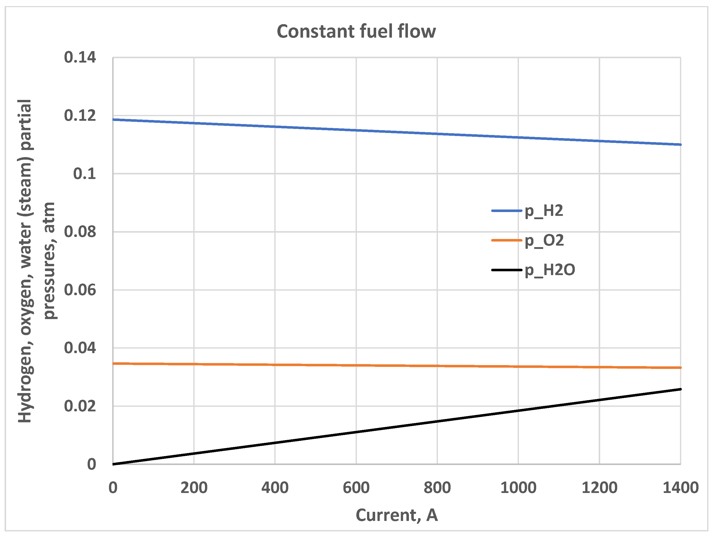
Figure 7.
Polarization curve when hydrogen and oxygen input flow rates are held constant; the Nernst loss and the ohmic loss are plotted separately.
Figure 7.
Polarization curve when hydrogen and oxygen input flow rates are held constant; the Nernst loss and the ohmic loss are plotted separately.

Figure 8.
Effect of the input hydrogen flow rate on polarization (both input flow rates are held constant, with the oxygen flow rate proportional to the hydrogen flow rate).
Figure 8.
Effect of the input hydrogen flow rate on polarization (both input flow rates are held constant, with the oxygen flow rate proportional to the hydrogen flow rate).

Figure 9.
Power-versus-current behavior (both input flow rates are held constant, with the oxygen flow rate proportional to the hydrogen flow rate).
Figure 9.
Power-versus-current behavior (both input flow rates are held constant, with the oxygen flow rate proportional to the hydrogen flow rate).
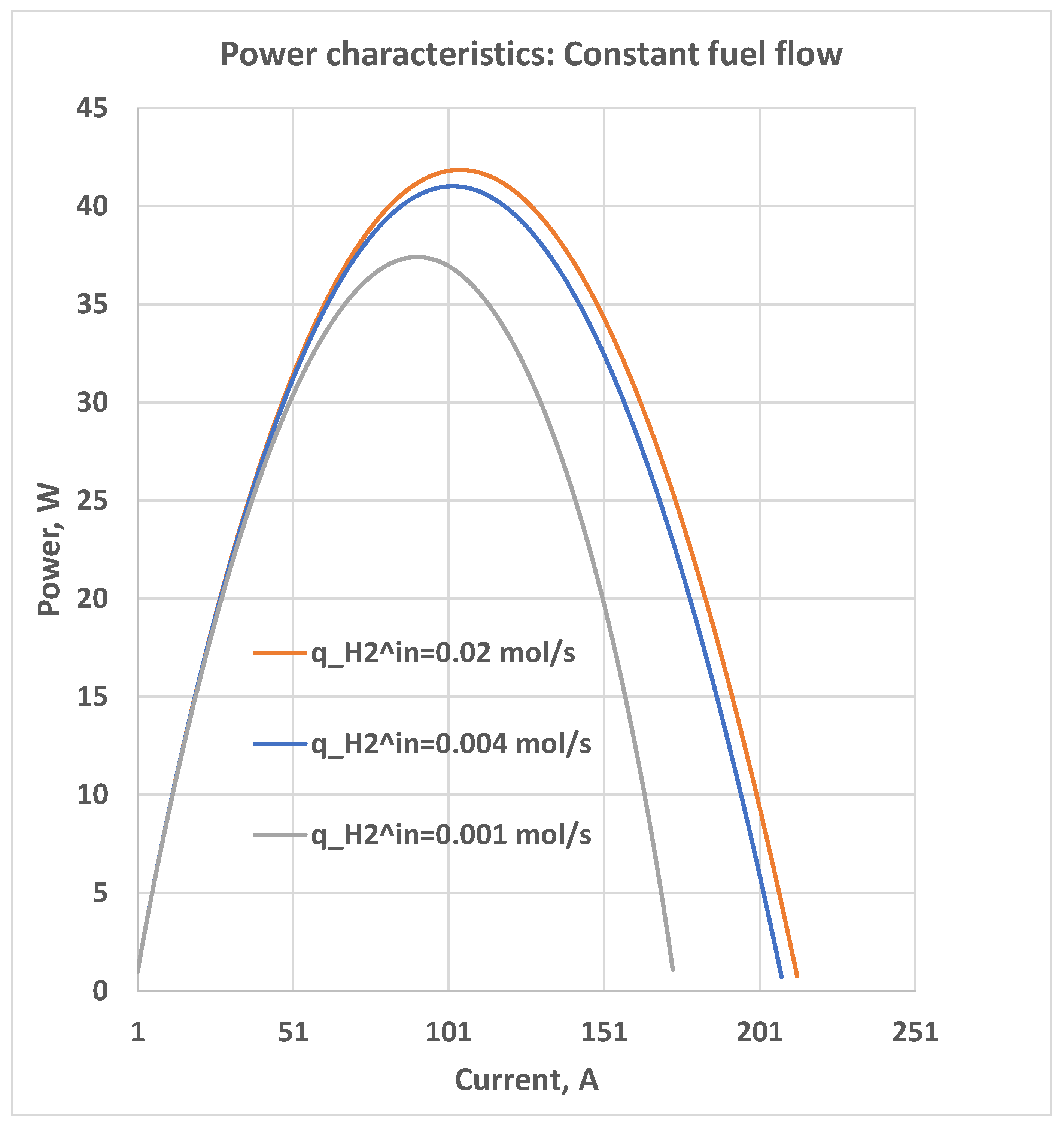
Figure 10.
Validation results for the constant fuel flow operation; mean absolute relative error = 3.96%.
Figure 10.
Validation results for the constant fuel flow operation; mean absolute relative error = 3.96%.

Figure 11.
Polarization characteristics (constant hydrogen flow and constant oxygen stochiometry); the Nernst loss is plotted separately.
Figure 11.
Polarization characteristics (constant hydrogen flow and constant oxygen stochiometry); the Nernst loss is plotted separately.
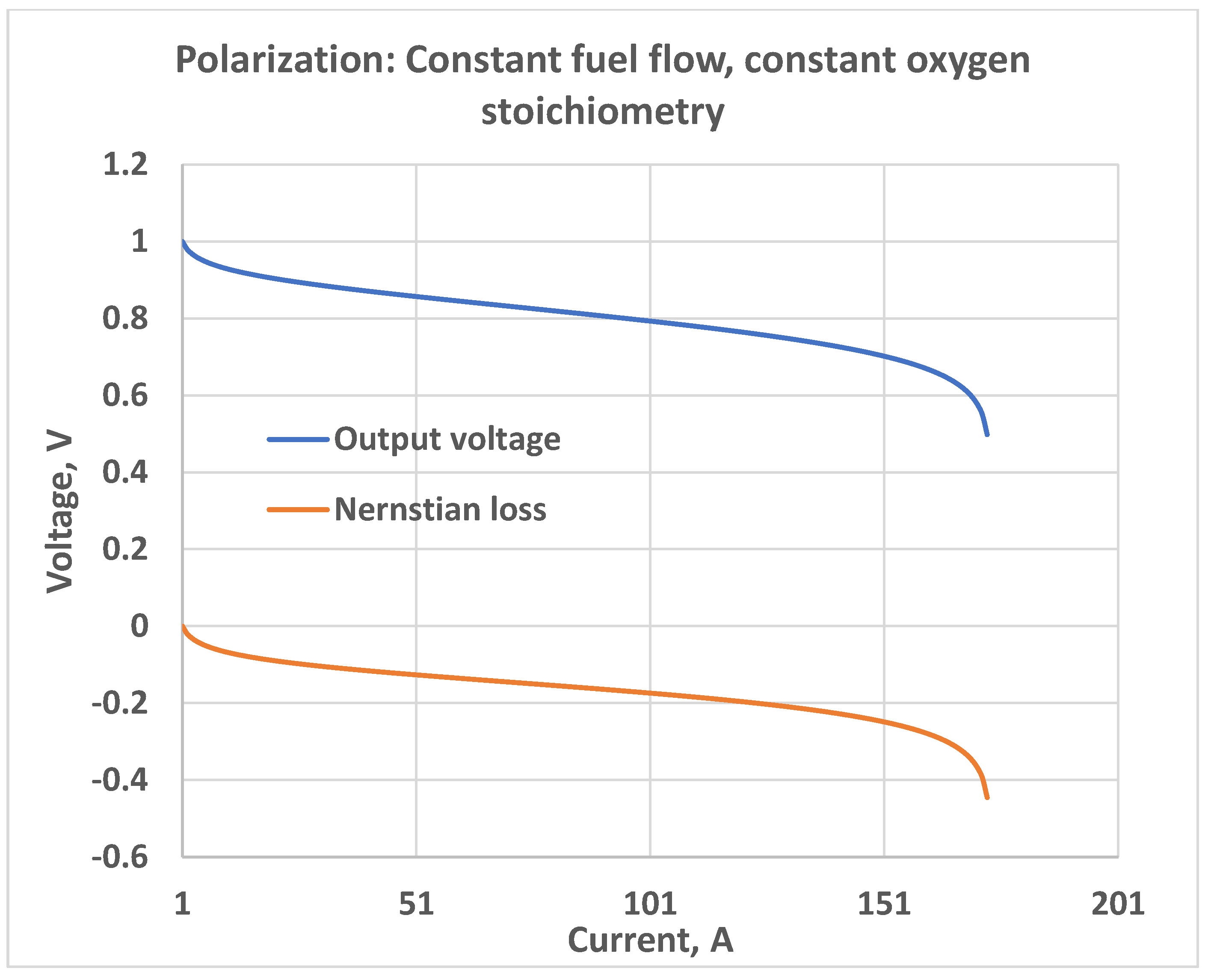
Figure 12.
Effect of the hydrogen flow rate on polarization (constant hydrogen flow and constant oxygen stochiometry).
Figure 12.
Effect of the hydrogen flow rate on polarization (constant hydrogen flow and constant oxygen stochiometry).
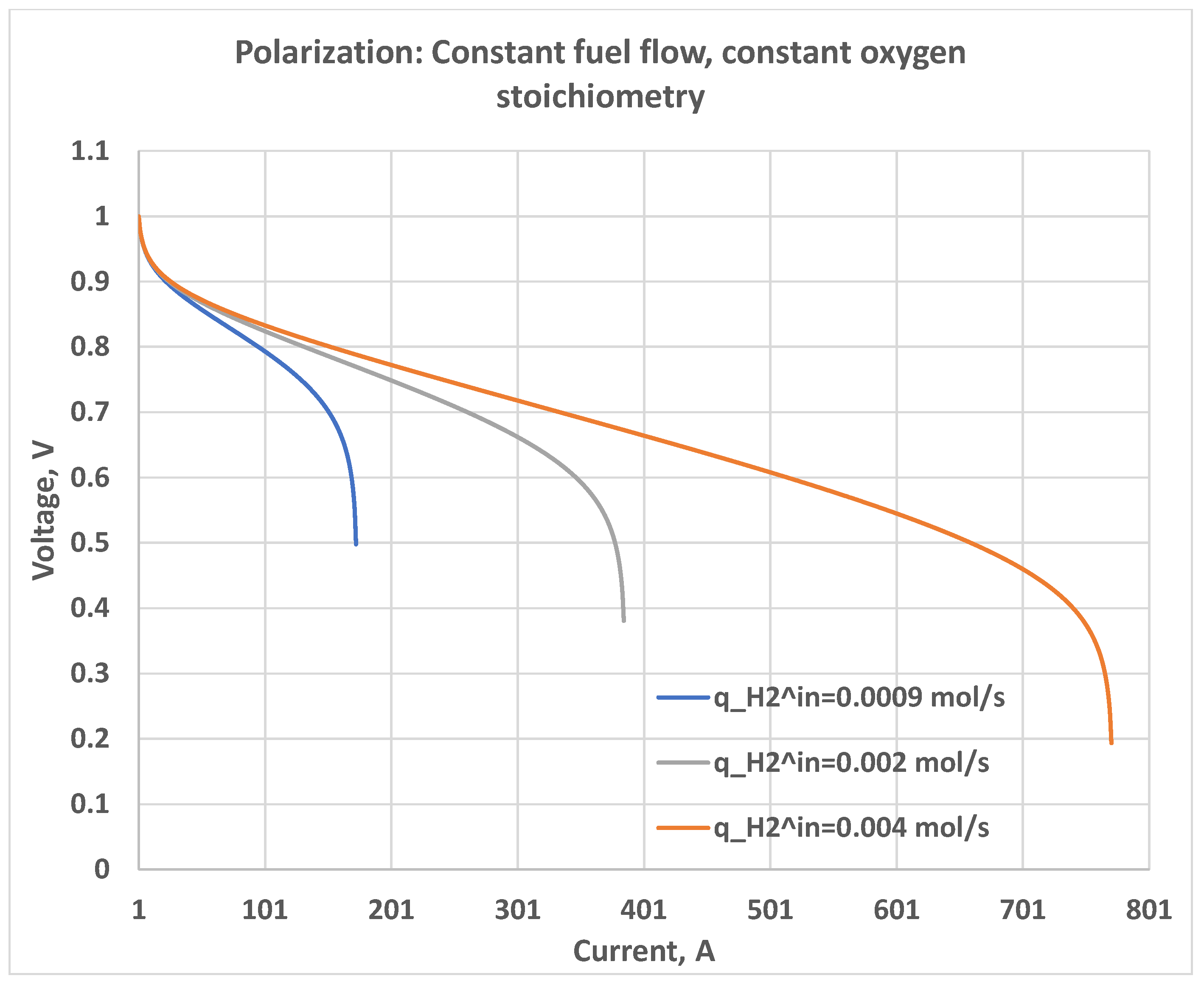
Figure 13.
Effect of the fuel flow rate on the power-versus-current behavior (constant hydrogen flow and constant oxygen stochiometry).
Figure 13.
Effect of the fuel flow rate on the power-versus-current behavior (constant hydrogen flow and constant oxygen stochiometry).


Table 1.
Numerical values of parameters and constants.
| Parameter | Value |
|---|---|
| T | 1273 K |
| u | 0.8 |
| 0.843 mol/(s·atm) | |
| 0.281 mol/(s·atm) | |
| 2.52 mol/(s·atm) | |
| r | 3.28125 × 10 |
| 1.145 | |
| n | 2 |
| Constants | |
| F | 96,485 Coulombs/mol |
| R | 8.31 J/(mol K) |
© 2019 by the author. Licensee MDPI, Basel, Switzerland. This article is an open access article distributed under the terms and conditions of the Creative Commons Attribution (CC BY) license (http://creativecommons.org/licenses/by/4.0/).
Share and Cite
MDPI and ACS Style
Chakraborty, U.K. A New Model for Constant Fuel Utilization and Constant Fuel Flow in Fuel Cells. Appl. Sci. 2019, 9, 1066. https://doi.org/10.3390/app9061066
AMA Style
Chakraborty UK. A New Model for Constant Fuel Utilization and Constant Fuel Flow in Fuel Cells. Applied Sciences. 2019; 9(6):1066. https://doi.org/10.3390/app9061066
Chicago/Turabian StyleChakraborty, Uday K. 2019. "A New Model for Constant Fuel Utilization and Constant Fuel Flow in Fuel Cells" Applied Sciences 9, no. 6: 1066. https://doi.org/10.3390/app9061066
Note that from the first issue of 2016, this journal uses article numbers instead of page numbers. See further details here.