Volumetric Tooth Wear Measurement of Scraper Conveyor Sprocket Using Shape from Focus-Based Method


1
College of Mechanical and Vehicle Engineering, Taiyuan University of Technology, Taiyuan 030024, China
2
Shanxi Key Laboratory of Fully Mechanized Coal Mining Equipment, Taiyuan 030024, China
3
School of Engineering and Computer Science, University of the Pacific, 3601 Pacific Ave., Stockton, CA 95211, USA
*
Author to whom correspondence should be addressed.
Appl. Sci. 2019, 9(6), 1084; https://doi.org/10.3390/app9061084
Submission received: 18 February 2019
/
Revised: 9 March 2019
/
Accepted: 11 March 2019
/
Published: 14 March 2019
(This article belongs to the Special Issue Intelligent Imaging and Analysis)
Abstract
:Volumetric tooth wear measurement is important to assess the life of scraper conveyor sprocket. A shape from focus-based method is used to measure scraper conveyor sprocket tooth wear. This method reduces the complexity of the process and improves the accuracy and efficiency of existing methods. A prototype set of sequence images taken by the camera facing the sprocket teeth is collected by controlling the fabricated track movement. In this method, a normal distribution operator image filtering is employed to improve the accuracy of an evaluation function value calculation. In order to detect noisy pixels, a normal operator is used, which involves with using a median filter to retain as much of the original image information as possible. In addition, an adaptive evaluation window selection method is proposed to address the difficulty associated with identifying an appropriate evaluation window to calculate the focused evaluation value. The shape and size of the evaluation window are autonomously determined using the correlation value of the grey scale co-occurrence matrix generated from the measured pixels’ neighbourhood pixels. A reverse engineering technique is used to quantitatively verify the shape volume recovery accuracy of different evaluation windows. The test results demonstrate that the proposed method can effectively measure sprocket teeth wear volume with an accuracy up to 97.23%.
1. Introduction
A scraper conveyor is the primary production and transportation equipment in a fully mechanized mining face [1]. In modern coal mining, the conveyor transports coal and provides hydraulic support and a walking track for the shearer. Therefore, its reliability directly affects the safety and production efficiency of modern coal mines. Sprockets are the core components of the chain drive system, which is the most important subsystem in the scraper conveyor [2]. Sprocket’s performance is directly related to the transport performance and service life of the scraper conveyor [3]. Sprockets contact chains directly; consequently, friction causes wear and excessive wear is the main form of sprocket failure and the main cause of scraper conveyor failure [4]. The sprocket conveyor chain may jump when it engages with the excessively worn sprocket; worn sprocket teeth may break, which affects the safe and efficient production of the coal mine, therefore, sprocket teeth wear analysis is required. Conventional wear measurement methods for scraper conveyor sprocket teeth include a weighing method, water volume measurement method, ANSYS analysis method [5] and wear monitoring [6]. Wang et al. [7] discussed the wear condition of a driving sprocket and the influence of wear on the sliding distance by taking the sliding speed and sliding distance of the meshing process as the index. Wang et al. [8] also analyzed the relationship between the deformation of a ring chain and driving sprocket wear by combining numerical analysis with experiments. However, these methods are not only tedious and time-consuming, they are also not sufficiently accurate or efficient.
The research of computer vision in industry field has attracted more and more attention of many researchers. Alverdi et al. [9] proposed a new way of using images to model the kerf profile in abrasive water jet milling. Qian et al. [10] presented an algorithm to compute the axis and generatrix focus on complex surfaces or irregular surfaces. A new monitoring technique for burr detection was proposed for the optimization of drill geometry and process parameters [11]. In addition, as a relatively simple and practical 3D reconstruction technology, shape from focus (SFF) has been applied to tool wear measurements [12,13], LCD/TFT (Liquid Crystal Display/Thin-Film Technology) display manufacturing [14] and grinding wheel surface morphology [15], etc.
To realize 3D surface topography restoration, in 1988, Darrell et al. [16] proposed using a Laplace operator-Gauss fitting method to search the clear frame of pixels in the sequence partial focus image according to image focusing information. In the 1990s, Nayar et al. [17,18] proposed an SFF-based method and obtained the height information of the corresponding surface of the window image by searching the image position corresponding to the maximum value of the focus evaluation function in the evaluation window. However, SFF suffers from some technical defects in pro-processing images and choosing evaluation function window size, thus developing methods to improve SFF accuracy has been the focus of ongoing research.
Many studies have proposed image pre-processing methods. For example, for wavelet transform, Karthikeyan et al. [19] introduced an effective denoising method for grey images using joint bilateral filtering. Khan et al. [20] introduced a new impulse noise detection algorithm that is based on Noise Ratio Estimation and a combination of K-means clustering and Non-Local Means based filter. An adaptive type-2 fuzzy filter is used to remove salt-and-pepper noise from images [21]. To improve the processing performance of image texture-free regions, Fan et al. [22] presented a shape focusing method combined with a 3D adjustable filter that considered edge response and image blurring. Liu et al. [23] proposed a graph Laplacian regularizer to preserve the inherent piecewise smoothness of depth, and this method demonstrated effective filtering. An iterative algorithm that combines stationary wavelet transform, bilateral filtering, Bayesian estimation and anisotropic diffusion filtering was used to reduce speckle noise in SAR images [24]. Khan et al. [25] designed a meshfree algorithm (Kansa technique) that uses a DTV method and a radial basis function approximation method to solve DTV-based model numerically to eliminate multiplicative noise in measurements. However, although the above methods can remove image noise to some extent, they change the grey-level information of non-noise areas of the image and affect the accuracy of 3D morphology restoration.
Mahmood et al. [26] analyzed the influence of different evaluation window sizes and noise types on the focusing evaluation function and concluded that, for different resolutions, the best evaluation window size for the same evaluation function was no single. Lee et al. [27,28] studied the focusing evaluation function window size. To determine the focusing evaluation function value, different standard window sizes were used to analyze the evaluation results of the size and shape of the focusing evaluation function window. Muhammad et al. [29] conducted 3D morphology restoration experiments on images collected using imaging equipment with different parameters and formulated the selection of the evaluation window. However, most of the above studies are based on the optimal size selection of a fixed square evaluation window without simultaneously optimizing both the shape and size of the window.
This paper presents an SFF-based method to measure scraper conveyor sprocket teeth wear efficiently. A specially designed device was used to collect a set of sprocket tooth wear sequence images. Normal distribution operator filtering, adaptive window evaluation and a Laplacian focusing evaluation function are applied to the obtained images. We obtain an initial depth map of the entire tooth wear surface. Then, a 3D shape recovery map is constructed to calculate the wear volume. This method improves measurement accuracy, can be operated remotely, and can be used to predict the life of the sprocket. More importantly, it is an efficient, fast and safe measurement method that provides data and technical support for coal mine production safety.
2. Measurement Scheme of Sprocket Teeth Wear of Scraper Conveyor
The scraper conveyor sprocket tooth wear measurement system based on SFF primarily comprises hardware and software. The hardware includes industrial cameras and control tracks, and the software includes 3D topography recovery and calculation of wear volume. The measurement process is summarised as follows. First, the sequence images of the tooth are collected using the hardware device. Then, the images are transmitted to the computer. Finally, the wear volume and geometric position of the sprocket teeth are obtained via 3D topography recovery and wear volume calculation.
2.1. Structure and Wear of Sprocket Teeth of Scraper Conveyor
A scraper conveyor sprocket [30] comprises a hub and sprocket teeth. The shape of the teeth is a geometric polygon, and each sprocket generally has five or seven teeth. The structure of the sprocket is shown in Figure 1.
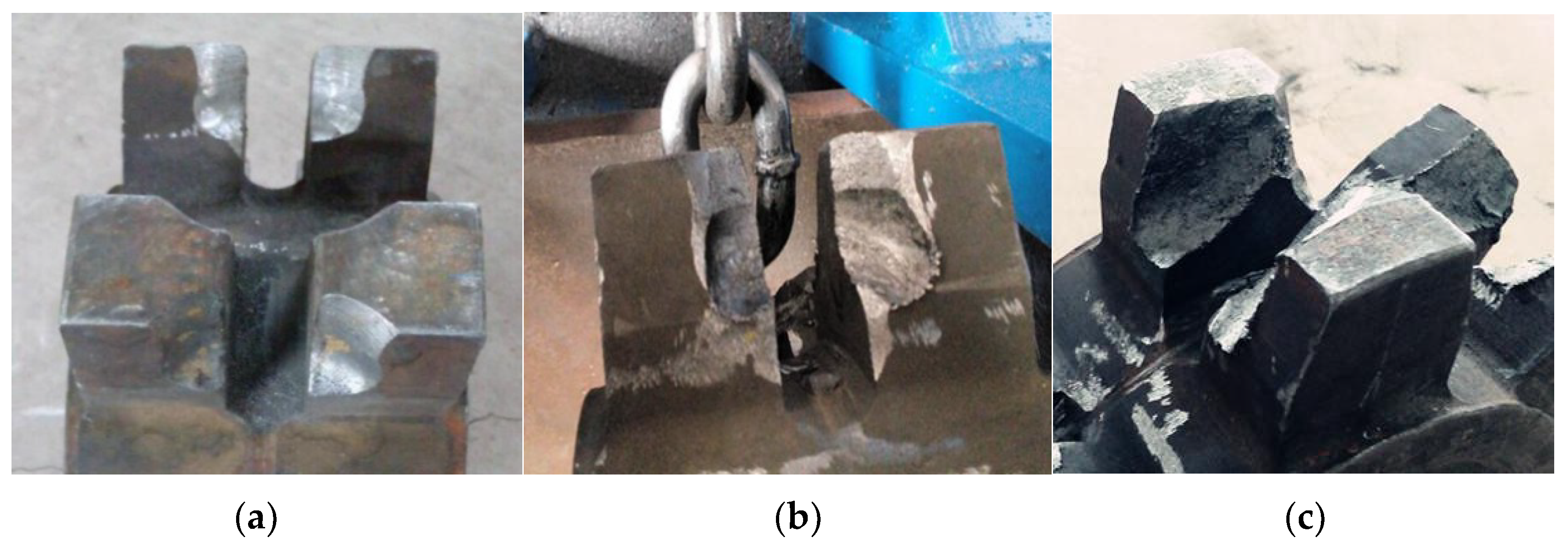
The working principle of the sprocket is to rotate the drive shaft to drive the hub to rotate, and the sprocket teeth engage with the circle chain. The different wear degrees of sprocket teeth are shown in Figure 2.
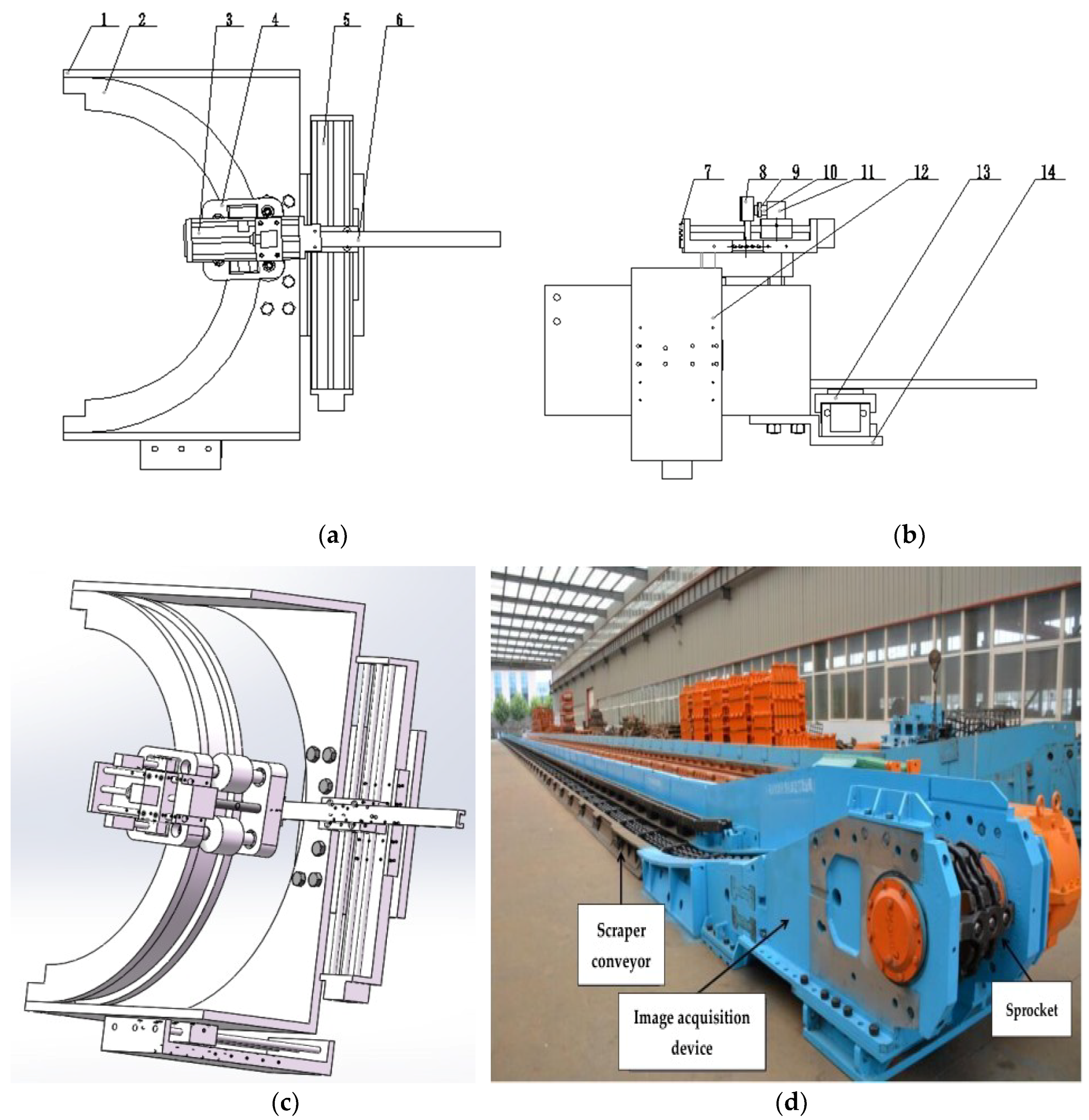
Figure 3a,b show the hardware device’s design, where 1: box; 2: circular track; 3: tooth radial motion module; 4: circular track slider; 5: circular slider driving module; 6: circular slider auxiliary track; 7: light receiver; 8: linear light; 9: ring light; 10: industrial lens; 11: industrial camera; 12: longitudinal motion module; 13: slider connection plate; 14: box connection plate.
The hardware device that measures sprocket wear includes position control, motion, centering, sequence image acquisition and other modules. The position control module primarily comprises a PLC unit and a driver unit, where the PLC unit includes different sub-units, such as longitudinal motion control, circumferential motion control, sprocket teeth radial motion control, camera control, linear light switch control, light receiver monitoring and ring light control. The motion module comprises a longitudinal motion unit, a circumferential motion unit and a radial sprocket teeth movement unit. The longitudinal movement unit includes a circular arc guide, a slider, a slider auxiliary guide rail and a slider drive module, and the centering module comprises a linear light unit and a light receiver unit. The sequence image acquisition module comprises a Charge Coupled Device CCD camera unit, a lens unit and an auxiliary light unit, and the other modules include support units and connection units. The structure of the sprocket wear measurement device is shown in Figure 3.
2.2. Wear Measurement Process Flow Chart
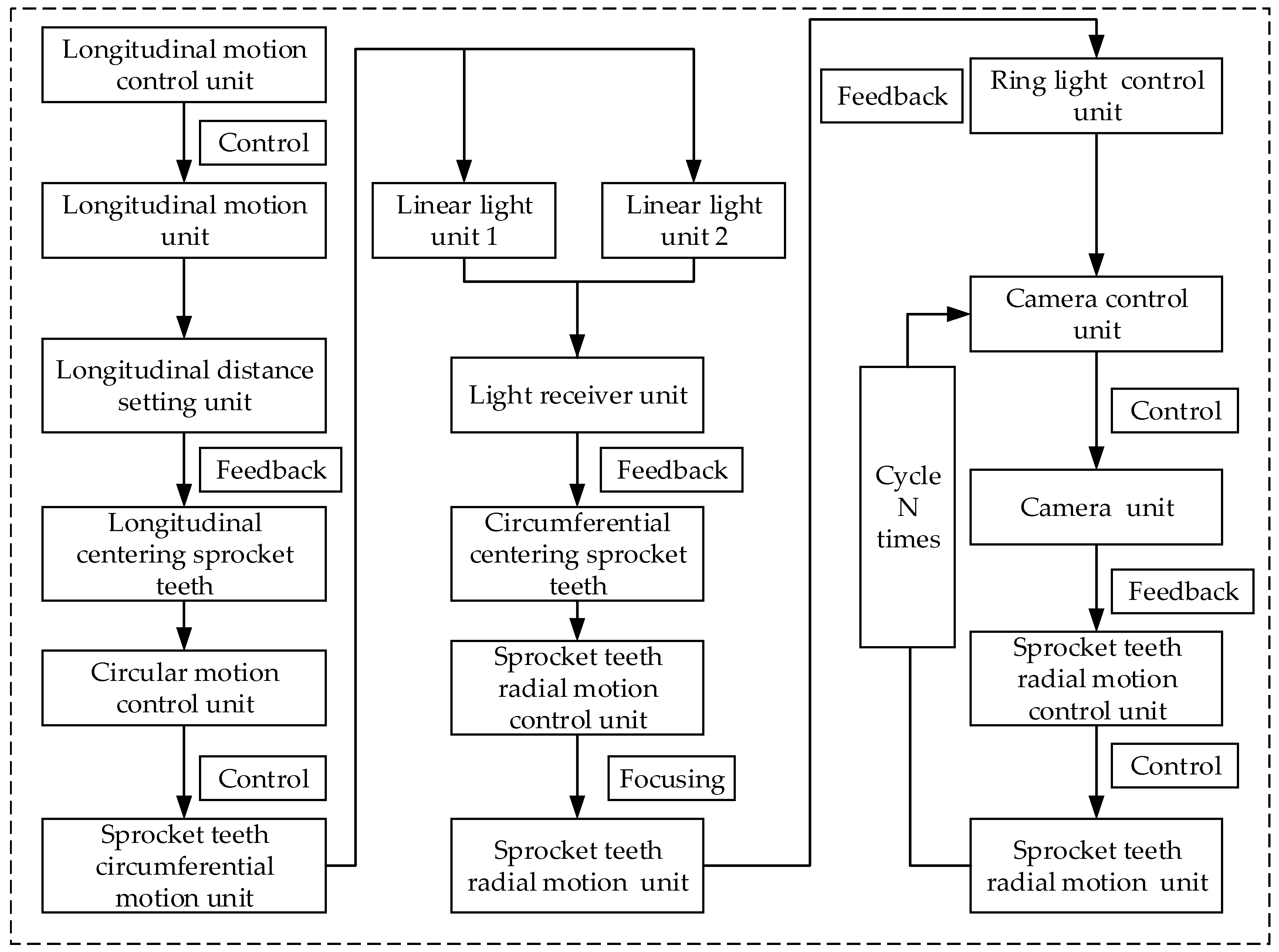
Figure 4 illustrates wear measurement process, which is addressed as follows.
Firstly, the longitudinal motion unit is driven to move in the longitudinal direction by the longitudinal motion control unit and stops when the moving distance reaches the set distance of the longitudinal distance unit. As a result, the camera unit is aligned with the longitudinal row of teeth. Secondly, the two linear light switches are turned on using linear light control unit, and the circular slider driving module is driven to move with the help of the circumferential control unit. When the light receiver unit simultaneously receives the signals from the two lights reflected back through the tooth surface, the circular slider driving module stops moving, which means that the camera unit is aligned with one of the teeth in the circumferential direction. Thirdly, the radial motion unit is driven to the designated focal length position by the sprocket tooth radial control unit, and the step distance is set to one N of the sprocket tooth height. The camera is driven by the camera control unit. Each step forward, the camera takes a picture, which cycles N times. The radial motion unit stops moving and returns to the original position, and then sequence image acquisition is completed.
The technical flow chart of the focused morphology restoration algorithm is shown in Figure 5.
First of all, the collected sequence images are read into the computer, and the field of view and resolution and cropping of all N-frame sequence images are transformed according to the proportional relationship of the target region of the N-frame sequence image. Normal distribution operator image filtering is used to filter the sequence images to obtain the same resolution. The pre-processed sequence images have N frames of the field of view. Therefore, N-frame pre-processed sequence image of the same resolution and field of view are obtained. Then, the clear pixel points of each pre-processed sequence image are extracted in order to construct a full-focus image. Then, the proposed adaptive method is used to select the focus evaluation window of any pixel in the full-focus image. The focus factor of each pixel in the pre-processed sequence image is calculated and the sequence image number corresponding to the maximum focus factor of all pixels in the full-focus image is obtained. The sequence image number is taken as the depth value of the corresponding pixels to form the initial depth map of the full-focus image. Next, a full-focus image is obtained with the help of image binarization, inversion, filling and contour recognition, and the object contour is extracted. The extracted object contour is applied to the initial depth map and the region outside the object contour is hollowed out to obtain a three-dimensional shape recovery map of the object. Lastly, the wear volume is calculated. The pixel equivalent and actual depth value of each pixel in the complete 3D topography is calculated, the tooth volume is determined using the limit method and the volume difference and wear volume between the recovered tooth model and the actual tooth model are calculated using the difference method.
3. Improved SFF
3.1. Principle of SFF
SFF is a method to recover a 3D topography from 2D sequence images [31]. SFF collects a series of partially-focused sequence images and obtains the depth information of each pixel based on focus information. Figure 6 shows a schematic diagram of an ideal optical system imaging principle. The object distance u, focal length f and distance v satisfy the relationship in an ideal optical imaging system. For a fixed-focus lens, the object point P forms a clear image point Pf on the focus plane through the optical system when the image sensor coincides with the focus plane. The object point P forms a blur circle of radius R on the image sensor when the image sensor does not coincide with the focus plane. Moreover, a greater distance between the image sensor and focus plane is results in greater R and the image points become more blurred. SFF must collect K-frame partial focus images Ik (k = 1, 2, …, K) of the measured surface along the optical axis, and these images contain the depth information of the entire measured surface.
To increase the robustness of the focus measure, the neighbourhood window U(x, y) of the pixel (x, y) is usually selected, rather than the pixel as the calculation object, and its size is w × w, this variable is expressed as follows.
where (ξ, η) represents the pixels in the neighbourhood U(x, y), and k is the image sequence number.
Focused images have more high-frequency components than blurred images. Therefore, the focusing degree is usually characterized by the sharpness of the pixel points and quantified using the focus measure in SFF.
When an evaluation function is selected, the evaluation function value sequence Ik(i, j) of pixel (i, j) can be obtained.
Since the clearest pixel can provide depth information of the corresponding surface element of the pixel, the depth of each pixel corresponding to the surface element can be obtained by obtaining each pixel in the image corresponding to the maximum focus volume. In this manner, the initial depth map of the measured surface is obtained. The formula is as follows:
Then, an approximation technique method is applied to refine the initial depth map.
3.2. Normal Distribution Operator Image Filtering
The influence of many factors like the image capturing hardware, surface texture and light inevitably introduces noise during data acquisition and transmission. Image noise greatly affects the accuracy of the value of the focus measure; it is necessary to use filtering techniques to eliminate them. During image acquisition, two main types of noise are produced: Gaussian noise and salt-and-pepper noise. Salt-and-pepper noise has a greater impact on the accuracy of the value of the focus measure [32]. The most prominent feature of salt-and-pepper noise is that the grey value of the noise pixels is different from those of its neighbourhood pixels. Therefore, the median filter is the best filtering method for this type of application. Median filtering is the most common filtering method; however, median filtering will change the grey value of all pixels in the image. To maintain the grey value of non-noise pixels in the image, the normal distribution operator is used to detect noise points. Then, median filtering is employed for the noise pixels, thereby retaining more of the original information contained in the image.
3.2.1. Principle of Normal Distribution
The normal distribution operator is a filtering algorithm based on normal distribution, which is defined as the probability distribution of random variable X obeying position parameter µ and scale parameter σ. The probability density formula is given as follows:
This random variable is referred to as a normal random variable, and the distribution it obeys is called a normal distribution, expressed as .
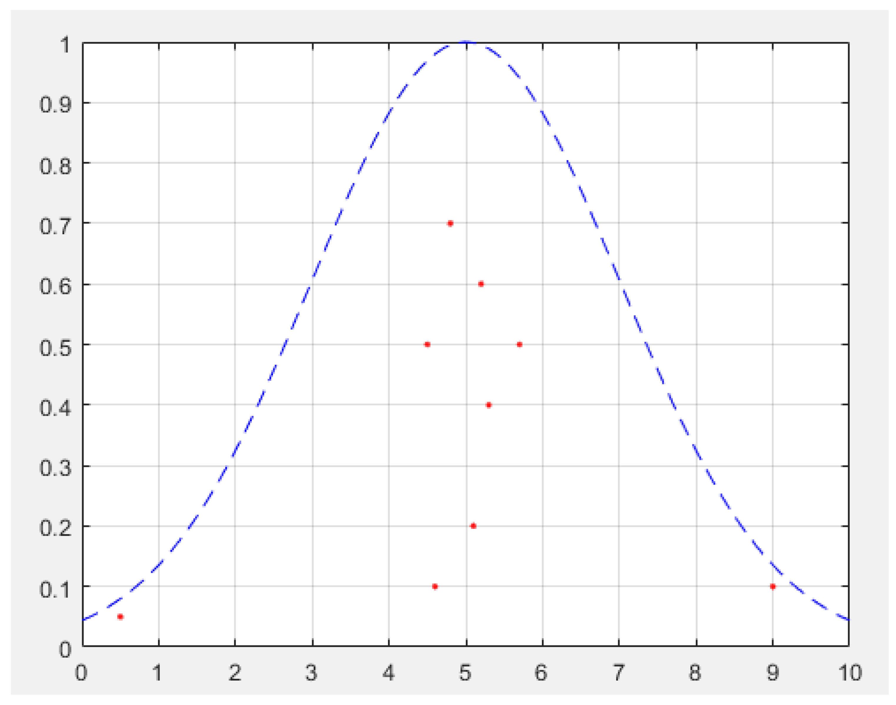
Figure 7 plots the normal distribution. According to the principle that salt-and-pepper noise is distant from the mean value, in the normal distribution with a mean of 5 and variance of 2, there are nine pixels in the 3 × 3 evaluation window, of which seven normal points are concentrated near the mean while the other noise points are distant from the mean. Use the median filter to replace the two abnormal points under the help of .
3.2.2. Noise Point Detection
In the 3 × 3 filter evaluation window, the grey value of pixel centre point (x, y) is f(x, y),and the pixel points in the centre pixel and its neighbourhood are represented as f11, f12, f13, f21, f22, f23, f31, f32 and f33, as shown in Figure 8.
According to the normal distribution principle and the Figure 8, the maximum and minimum of the nine points in the 3 × 3 filter evaluation window are removed. The mean and variance of the remaining seven points are taken as µ and σ, which are expressed as follows.
From the above formula, the average of the seven points is calculated as the mean and variance as the variance of the normal distribution, where K is the threshold. The centre pixel is a non-noise point when the absolute value of the difference between the centre pixel and the mean is in the Kσ range and do not change its grey value. By taking the centre pixel as a non-noise point, the absolute value of the difference between the centre pixel and the mean is not in the Kσ range. After median filtering, the original grey value is replaced with Med. The grey value obtained after filtering is , and the formula is given as follows.
An experiment proved that the filtering effect was best when threshold K was set to 2.2.
3.2.3. Algorithm Verification and Evaluation Analyzes
To verify the feasibility of the operator filtering, three images of a vegetable, a ball and a human, respectively, were selected as test objects. (These images, shown in Figure 9, were chosen from a book named Detailed Explanation of Image Processing Example in MATLAB.) Salt-and-pepper noise with a density of 0.01 was added to the images, and we performed median filtering and normal distribution operator filtering on the noise images (threshold value K: 2.2).
To evaluate the quality of median filtering and normal distribution operator filtering quantitatively, we selected correlation and the peak signal-to-noise ratio (PSNR) as quantitative assessment criteria. Correlation was used to evaluate the similarity between the reference and real data, where a greater correlation value indicates that the reference data are more consistent with the real data. PSNR was used to measure image quality after filtering, where a greater PSNR value indicates less image distortion. The formulas for correlation and PSNR are given follows.
In Equations (10)–(12), M represents the width of the image, N denotes the height of the image, I’(x, y) stands for the actual grey value of the pixel point (x, y), and represents the estimated average grey value for all pixels in the image. While I(x, y) denotes the grey value of the pixels (x, y) after filtering, and stands for the estimated average grey value for all pixels after filtering in the image, MSE represents the mean square error.
Figure 10 shows the noise and filter processing results with a density of 0.01. Here, the first, second and third columns show images with density of 0.01, images processed using median filtering and images processed using normal distribution operator filtering, respectively. As shown in Figure 10a, the images contain large number of errors. Note that these errors are reduced significantly by filtering the noise image. In addition, the median filtered images (Figure 10b) are more blurred than the original image and the filtering effect is poor. However, images obtained via normal operator filter processing are closer in appearance to the corresponding original images.
Table 1 shows the correlation and root mean squared error (RMSE) data for three sequence images processed by adding noise and by applying median filtering and normal distribution operator filtering. As can be seen, the correlation and RMSE values obtained by the two filtering methods are greater than those obtained with the noisy image sequence. Furthermore, the increase to these values is more obvious with normal distribution operator filtering. Both filtering methods improve the accuracy of image filtering; however, the results demonstrate that normal distribution operator filtering is better.
3.3. Proposed Adaptive Window Selection Method
3.3.1. Grey-Level Co-Occurrence Matrix and Its Correlation Features
The grey-level co-occurrence matrix [33] is a matrix function of the distance and angle between pixels. This measure reflects the comprehensive information on the direction, interval, amplitude and speed of the image through the correlation between a certain distance of the image and the two-pixel grey of a certain direction.
The galactic co-occurrence matrix [34,35,36] is defined as the probability from grey-level i to a fixed position d = (Dx, Dy) to the grey-level j. The grey-level co-occurrence matrix is denoted by Pd(i, j)(i, j = 0, 1, 2,…, L − 1), where i and j represent the grey scale values of two pixels, respectively, and L denotes the grey level of the image. The spatial relationship d between two pixels is shown in Figure 11, where θ is the direction of generation of the grey-level co-occurrence matrix.
When d is selected, the grey-level co-occurrence matrix Pd under a certain relation d is generated.
Usually, scalars can be used to describe the characteristics of the grey-level co-occurrence matrix. The correlation features are used to measure the degree of similarity in the horizontal or vertical direction of the grey level of the image, and the magnitude of the value reflects the approximate degree of the local grey level correlation. The larger the correlation value is, the larger the correlation of the local grey level as shown in Equation (14).
Here, µ1, µ2, σ1, and σ2 are respectively defined as follows:
where i and j represent the grey values of two pixels, L is the grey level of the image, and d represents the spatial position relationship of two pixels.
3.3.2. Calculation of the Shape and Size of the Evaluation Window
For any pixel (x, y) in the image, the horizontal left neighbourhood N h1 (x, y), the horizontal right neighbourhood N h2 (x, y), the vertical neighbourhood N v1 (x, y) and the vertical lower neighbourhood N v2 (x, y) are respectively in Equations (19)–(22).
For an overly large m, the neighbourhood of the pixel exceeds the range of the acceptable evaluation window. Taking m = 3, the corresponding maximum evaluation window size is 7 × 7 pixels. In the horizontal direction, a grey-level co-occurrence matrix Pd1(k1) with a distance from the centre pixel point (x, y) and an angle of 180° is generated with the pixel horizontal left neighbourhood N h1 (x, y), and the correlation eigenvalue Cor(k1) corresponding to the grey-level co-occurrence matrix is obtained. A grey-level co-occurrence matrix Pd2(k2) with a distance from the centre pixel point (x, y) and an angle of 0° is generated with the pixel horizontal right neighbourhood N h2 (x, y), and the correlation eigenvalue Cor(k2) corresponding to the grey-level co-occurrence matrix is obtained. Similarly, a grey-level co-occurrence matrix Pd3(k3) with a distance from the centre pixel point (x, y) and an angle of 270° is generated with the pixel vertical upper neighbourhood N v1 (x, y), and the correlation eigenvalue Cor(k3) corresponding to the grey-level co-occurrence matrix is obtained. A grey-level co-occurrence matrix Pd4(k4) with a distance from the centre pixel point (x, y) and an angle of 90° is generated with the pixel vertical lower neighbourhood N v2 (x, y), and the correlation eigenvalue Cor(k4) corresponding to the grey-level co-occurrence matrix is obtained.
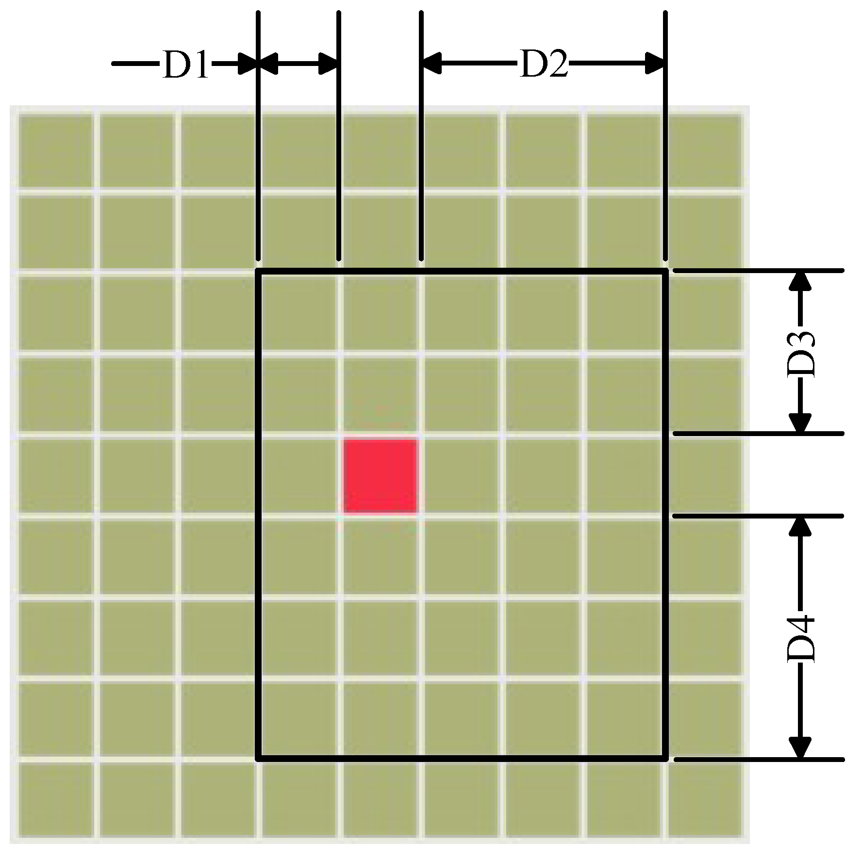
To find the maximum correlation pixels of the four neighbourhoods of the centre pixels (x, y), the pixels corresponding to the maximum correlation eigenvalues of the grey-level co-occurrence matrix in each direction are taken as the maximum relevant pixel, and the maximum correlation distances D1, D2, D3 and D4 of the centre pixel in the four squares’ directions are calculated by Equations (23)–(26).
The maximum correlation distances D1, D2, D3 and D4 of the centre pixels in four directions can be used to determine the shape of the rectangular evaluation window of the pixel, and the width Lx = D1 + D2 + 1 and height Ly = D3 + D4 + 1 of the neighbourhood window are obtained. A diagram of the neighbourhood window is shown in Figure 12.
3.4. Main Procedures of the Improved SFF Algorithm
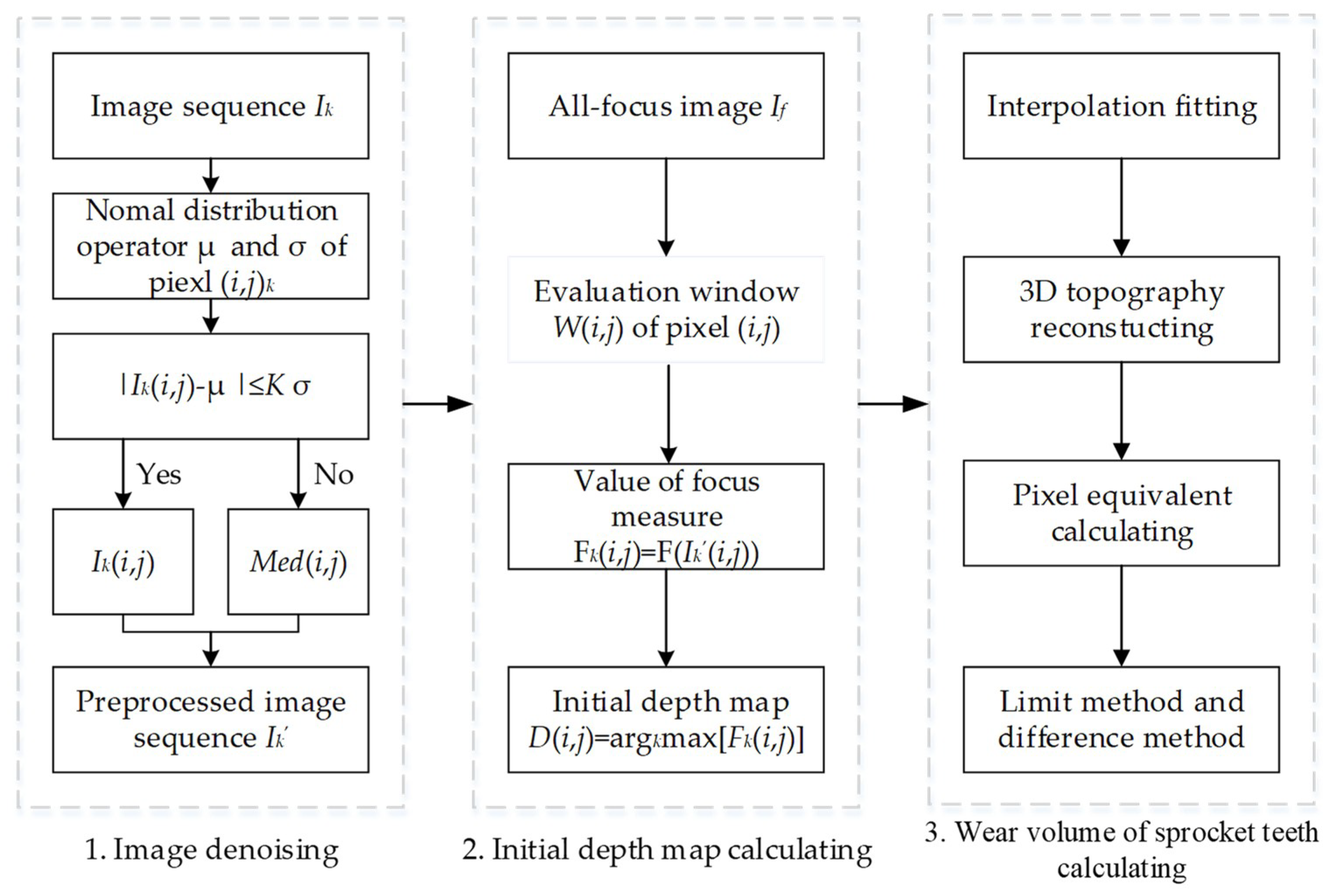
According to the above stated method, the process of the improved SFF algorithm is shown in Figure 13. The improved SFF algorithm has three main steps, consisting of the original sequence image de-noising, the initial depth map calculation, and the initial depth map refining. First, the image sequence Ik is detected by using the normal distribution operator, and a new grey value is assigned to a pixel determined as noise by using the median filtering method. Otherwise, the original pixel grey level is kept unchanged, and the preprocessed image sequence I’k is obtained (the threshold value K is 2.2.) Then, the Laplacian operator is used to extract the clear pixels in the preprocessed sequence image I’k of each frame to construct an all-focus image If. The adaptive evaluation window selection method is used to determine the evaluation window W(i, j) of each pixel (i, j) in the fully focused image; then, it calculates the focus measure value of each pixel of the image sequence I’k, and find the image number corresponding to the maximum focus measure value of each pixel (i, j) to obtain the initial depth map. Lastly, using the depth valued of all pixels, the 3D topography is reconstructed via interpolation. The pixel equivalent is calculated according to the width and height of the pixel and the tooth size of the 3D topography. The limit method is employed to obtain the 3D volume of the worn sprocket teeth and is combined with difference method to obtain the tooth wear volume.
3.5. Test Results and Analysis
To verify the effectiveness of the algorithm, three synthetic objects, i.e., spherical surface, a complex surface and a simple surface, were used as test virtual objects, as shown in Figure 14. In addition, an analogue camera imaging mathematical model was used to create differently focused image sequences of 100 frames, corresponding to the three virtual models, which are 360 × 360 [37].
Salt-and-pepper noise with a density of 0.01 was added to the images of the 10th, 20th, 30th, 40th, 50th, 60th, 70th, 80th, 90th, and 100th frames of the spherical, complex, and simple surface models. The three focus measures FSML, FTEN [38], and FGLV [39] were selected as the test measures. Windows with a size of 3 × 3, 5 × 5, 7 × 7, and the adaptive evaluation window proposed in this paper were used to conduct a 3D morphological recovery test for the image sequences generated using the three models.
Figure 15, Figure 16 and Figure 17 show the initial depth maps of the three models when FSML, FTEN, and FGLV were chosen as the focus evaluation functions, and different evaluation windows were applied. Columns one to four in the figure are the three models of the 3D morphologies that were recovered and generated by using 3 × 3, 5 × 5, and 7 × 7 windows and the adaptive evaluation window proposed in this paper. Figures show that when the evaluation window is 3 × 3, the 3D surface topography of all three recovered models appears to have more error values. In comparing the recovery results of the three models, when the surface of the recovery object is smooth and we appropriately increase the evaluation window, the three types of evaluation functions can obtain accurate 3D topographic images. As the surface geometry tends to be complex, increasing the evaluation window does not obviously reduce the error effect. As can be seen from the recovery results of the spherical surfaces in figures, the error of the adaptive evaluation window is obviously less than that of the other evaluation windows, which indicates that the adaptive evaluation window in this algorithm is also effective for noisy image sequences.
The test compares the actual morphology with the morphology obtained through the test using qualitative observation. Then, the recovery is quantitatively evaluated using the assessment criteria, RMSE and correlation [40]. RMSE and correlation are used to evaluate the error and similarity between the reference data and the real data, respectively. The smaller the RMSE value, the smaller the error between the reference data and the real data. The greater the correlation value, the more consistent the reference data is with the real data. The calculation methods of RMSE and correlation are addressed in Equations (27) and (28).
In Equations (27) and (28), M represents the number of rows of the image, N denotes the columns of the image, D′ (i, j) stands for the actual depth of the pixel point (i, j), and represents the average depth value for all pixels in the image. While D (i, j) stands for the estimated depth of the pixel point (i, j), and represents the estimated average depth value for all pixels in the image.
It can be seen from the 3D morphology diagram of the three models reconstructed by the three evaluation functions in the Figure 15, Figure 16 and Figure 17, Table 2, Table 3 and Table 4 show the RMSE and correlation data of the models’ morphological recovery results of the spherical surface, complex surface and simple surface when FSML, FTEN, and FGLV are chosen as evaluation functions.
According to the RMSE data in the table, when the evaluation window is 3 × 3, the RMSE values restored by the three evaluation functions are the largest, and the larger the evaluation window, the smaller the RMSE value. For example, in the surface morphology recovery using the FSML evaluation function, the RMSE values of the conical surface, simple surface and complex surface obtained by the adaptive window are 0.0036, 0.0256 and 0.0121, in contrast of 3 × 3, 5 × 5, 7 × 7, window, the RMSE value of the adaptive window is minimal. This finding shows that, when the evaluation window is smaller, there are more error values in the recovery results. Furthermore, as the evaluation window increases, the error values gradually decrease, and the effect of the adaptive window is better when the image tends to be smooth. When the evaluation window is 3 × 3, the correlation values restored by the three evaluation functions are significantly smaller than those of other evaluation windows. In addition, the correlation value of the adaptive evaluation window in this algorithm is larger compared to a fixed-size evaluation window. This phenomenon is more obvious when surface geometry is spherical. For instance, in the surface topography recovery of spherical surfaces using the FSML evaluation function, the Cor values of 3 × 3, 5 × 5, 7 × 7 and adaptive windows are 0.9823, 0.9899, 0.9942 and 0.9985 respectively. The Cor value of adaptive windows is at least 0.4% higher. This finding shows that the 3D topographic map reconstructed with the adaptive evaluation window of this algorithm is closer to the original surface. The more complex the surface topography, the greater the advantage of an adaptive evaluation window.
On the basis of the qualitative observation and comparison and the quantitative data analysis, when we restore the 3D image sequence with noise, compared to a fixed-size evaluation window, regardless of the evaluation function we choose, the error value of the recovery result, the coincidence degree of the 3D image or the original surface morphology, employing the adaptive evaluation window provides good results. Therefore, this algorithm is also feasible for the restoration of the 3D topography of noisy images.
4. Application Example
The above is a test of three virtual models, which shows that the algorithm is effective for virtual models. In addition, to verify the effectiveness of this algorithm in the physical 3D surface morphology restoration of actual solids, a scraper conveyor sprocket tooth is selected as recovery objects, and image acquisition device designed in this paper is used to sequentially collect 100 frames of 1980 × 1114 object images. Figure 18 is an actual entity of sprocket teeth and the 3D model of the sprocket teeth.
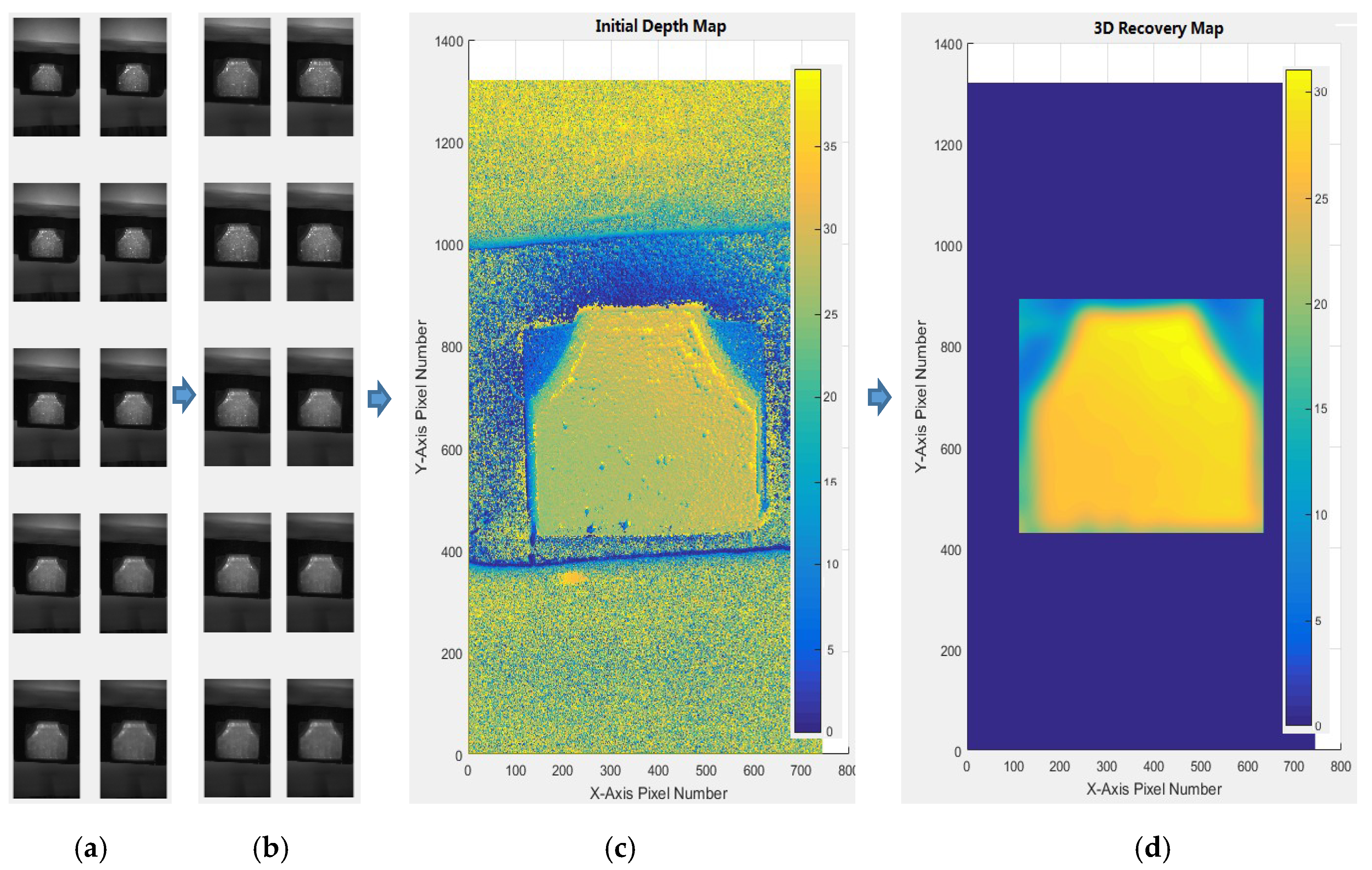
Firstly, image cropping and filtering are performed on the collected 100 frame sequential image. Then, different evaluation windows, evaluation function and peak positioning technology are used to acquire the initial depth map of sprocket tooth. Finally, the background area is removed by image segmentation technology, and the 3D recovery map of sprocket tooth is obtained. Figure 19a,b are the partial original images and pre-processed images of 100 frame sequential images respectively. Figure 19c,d are the initial depth map and the 3D recovery map of sprocket teeth respectively.
To compare the recovery accuracy of adaptive window with other fixed-size windows, the morphology recovery test is carried out. FSML focus measures is selected in this test, and 3 × 3, 5 × 5, and 7 × 7 windows and the adaptive evaluation window proposed in this paper are used to reconstruct the 3D image of the sprocket tooth. The recovery effect is qualitatively evaluated based on observations, and the actual appearance and the shape obtained are compared in the test. Figure 19 shows the initial depth map of the sprocket tooth. The row from left to right are restored by FSML focus evaluation operator using the evaluation windows of size 3 × 3, 5 × 5 and 7 × 7 and the adaptive window, respectively.
We can observe form Figure 20, when the evaluation window is 3 × 3, on the surface of the part, there are many error values in the 3D morphologies restored using FSML evaluation functions. With the increase in the evaluation window, the overall image tends to be smooth, the error value is gradually reduced, and the surface morphology is closer to the surface of the original part. When we select the adaptive evaluation window, the surface profile of the part is the clearest and the surface is smooth. In particular, the pits on the surface of the part are retained, and compared with the other four evaluation windows, the recovery effect is the best. In summary, the evaluation window size has a great influence on the result of the appearance recovery when the 3D surface morphology of the sprocket tooth is restored. An undersized evaluation window is not conducive to recovery results. Compared to the traditional fixed-size evaluation window, the adaptive evaluation window can effectively reduce the error value and preserve the surface texture details.
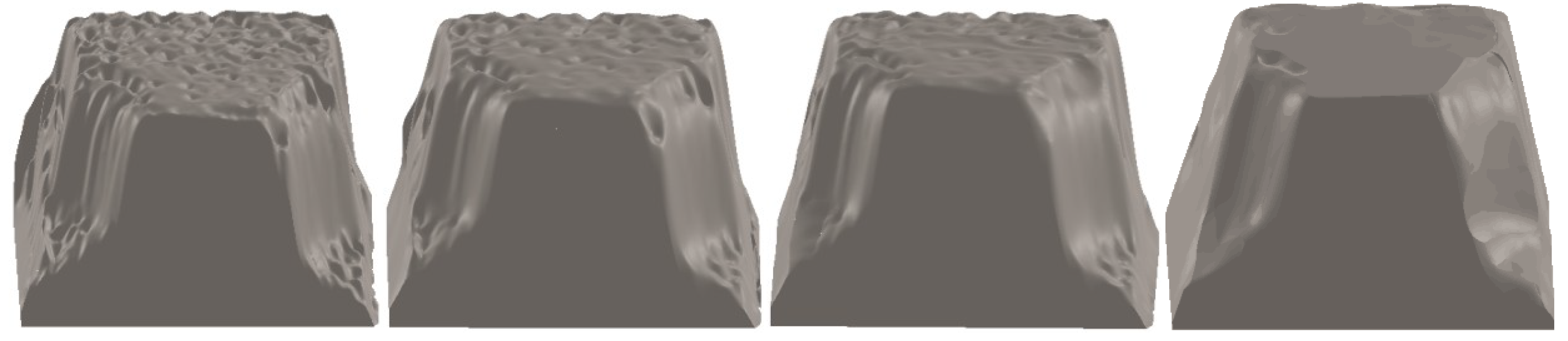
To further quantitatively verify the accuracy of the adaptive evaluation window, the degree of similarity between the reconstructed 3D model and the original model was deeply analyzed, and a further experiment was carried out. First, MATLAB (The MathWorks Inc., Natick, MA, ver.2015b) software was used to extract the 3D surface point data in Figure 20, and the extracted point data was saved in the txt folder; then, the IMAGEWARE software was used to read the point data under the txt folder to form a point cloud image, and reverse engineering was applied to restore the point cloud to a curved surface. Finally, the surface was formed to a 3D model in the SolidWorks software, as shown in Figure 21; from left to right, the reconstructed 3D entities of the 3 × 3, 5 × 5, 7 × 7 windows and the adaptive evaluation window were obtained by the FSML focus evaluation operator.
The reconstructed 3D entity coincides with the centre of gravity of the original 3D model established in Figure 18 and performs a Boolean operation to obtain a public part reconstructed from the original 3D entity, as shown in Figure 22, from left to right; the public part of the 3 × 3, 5 × 5, 7 × 7. windows and the adaptive evaluation window are obtained from the FSML focus evaluation operator.
It can be seen from the above figure that, when the evaluation window is 3 × 3, the surface of the common part has the largest number of pits and the largest error value, and with the increase of evaluation window, the surface of public entities tends to be smooth, while the adaptive evaluation window has the best smoothness and the lowest error value.
The larger the volume of the public part, the greater the accuracy of recovery; therefore, the accuracy of recovery can be expressed by the following formula:
i takes values from 1–4, SolidWorks software measures the volume of original model (V0 = 32511.83 mm3), Vi represents the volume of 3D entities reconstructed by different evaluation windows by FSML focusing evaluation operator, and V0i represents the volume of the 3D entities reconstructed by different evaluation windows and common entities of original models by the FSML focusing evaluation operator and calculates the volume evaluation results of metal entity reconstructed by FSML in different evaluation windows, as shown in Table 5.
It can be seen from Table 5 that the evaluation window is 5 × 5, 7 × 7 and the adaptive evaluation window obtains an image volume, which is basically the same as the volume of the common part. With the increase of the evaluation window, the volume of the overlapping part increases, the volume of the common part of the adaptive evaluation window reaches the maximum, i.e., 31833.45mm3, and the recovery accuracy of the adaptive evaluation window reaches 97.23%.
According to the 3D shape restoration test results of the scraper conveyor sprocket tooth, the focus value obtained using the adaptive evaluation window is more accurate than the traditional fixed-size square evaluation window when we qualitatively and quantitatively analyze the test results, and it is also feasible to combine the normal distribution operator filtering method in this algorithm.
5. Conclusions
An SFF-based method was proposed in order to effectively measure the wear volume of sprocket teeth in a scraper conveyor; the following conclusions were drawn:
- A hardware device for volumetric tooth wear measurement was designed and assembled to collect sequential images of sprocket teeth, which provides a way for images acquisition of measuring the wear volume of sprocket teeth in a scraper conveyor.
- A normal distribution operator image filtering method was presented, which only filters the noise points in the image without changing the grey value of the non-noise point pixels. Therefore, compared with the traditional filtering method, more original information of the image is retained to a large extent.
- An adaptive evaluation window selection method was proposed. A focused morphology restoration algorithm based on the normal distribution operator-region pixel reconstruction was formed, which not only effectively eliminates the error of restoration accuracy caused by noise interference, but also satisfies the requirement of peak location. Therefore, both the accuracy and effectiveness of morphology restoration has been improved.
- Compared to other focused 3D restoration methods, the proposed methods can effectively measure the wear volume of sprocket teeth with a recovery accuracy of up to 97.23%.
- In order to further improve the accuracy of this method and expand the scope of application, we will consider the advantages of structured light [41] for further research.
Author Contributions
H.D. proposed the method; Y.L. performed the experiments and analyzed the data; J.L. contributed method guidance and language modification; H.D. wrote the paper.
Funding
This work was funded by the Shanxi Science and Technology Foundation Condition Platform Project, grant 201805D141002 and the Joint Training Base for Postgraduate Students in Shanxi Province, grant 2018JD15.
Acknowledgments
Thanks are due to Shanxi Coal Mine Machinery Manufacturing Co., Ltd. for providing experimental equipment and application environment.
Conflicts of Interest
The authors declare no conflicts of interest.
References
- Dolipski, M.; Remiorz, E.; Sobota, P. Determination of dynamic loads of sprocket drum teeth and seats by means of a mathematical model of the longwall conveyor. Arch. Min. Sci. 2012, 57, 1101–1119. [Google Scholar]
- Jiang, S.B.; Zeng, Q.L.; Wang, G.; Gao, K.D.; Wang, Q.Y.; Hidenori, K. Contact analysis of chain drive in scraper conveyor based on dynamic meshing properties. Int. J. Simul. Model. 2018, 17, 81–91. [Google Scholar] [CrossRef]
- Sobota, P. Determination of the friction work of a link chain interworking with a sprocket drum. Arch. Min. Sci. 2013, 58, 805–822. [Google Scholar]
- Ren, F.; Shi, A.Q.; Yang, Z.J. Research on load identification of mine hoist based on improved support vector machine. Trans. Can. Soc. Mech. Eng. 2018, 42, 201–210. [Google Scholar] [CrossRef]
- Põdra, P.; Andersson, S. Finite element analysis wear simulation of a conical spinning contact considering surface topography. Wear 1999, 224, 13–21. [Google Scholar] [CrossRef]
- China University of Ming and Technology. A Monitoring Device and Method for Abrasion of Scraper Conveyor Sprocket Tooth Wear. CN Patent CN201610325560, 17 August 2016. [Google Scholar]
- Wang, S.P.; Yang, Z.J.; Wang, X.W. Wear of driving sprocket for scraper convoy and mechanical behaviors at meshing progress. J. China Coal Soc. 2014, 39, 166–171. [Google Scholar]
- Wang, S.; Yang, Z.; Wang, X. Relationship between Round Link Chain Deformation and Worn Sprocket. China Mech. Eng. 2014, 25, 1586–1590. [Google Scholar]
- Alberdi, A.; Rivero, A.; López de Lacalle, L.N.; Etxeverria, I.; Suárez, A. Effect of process parameter on the kerf geometry in abrasive water jet milling. Int. J. Adv. Manuf. Technol. 2010, 51, 467–480. [Google Scholar] [CrossRef]
- Qian, X.; Huang, X. Reconstrction of surfaces of revolution with partial sampling. J. Comput. Appl. Math. 2004, 163, 211–217. [Google Scholar] [CrossRef]
- Peña, B.; Aramendi, G.; Rivero, A.; López de Lacalle, L.N. Monitoring of drilling for burr detection using spindle torque. Int. J. Mach. Tools Manuf. 2005, 45, 1614–1621. [Google Scholar] [CrossRef]
- Xiong, G.X.; Liu, J.C.; Avila, A. Cutting tool wear measurement by using active contour model based image processing. In Proceedings of the IEEE International Conference on Mechatronics and Automation, Beijing, China, 7–10 August 2011; pp. 670–675. [Google Scholar]
- Liu, J.C.; Xiong, G.X. Study on Volumetric tool wear measurement using image processing. Appl. Mech. Mater. Manuf. 2014, 670–671, 1194–1199. [Google Scholar] [CrossRef]
- Ahmad, M.; Choi, T.S. Application of three dimensional shape from Image focus in LCD/TFT displays Manufacturing. IEEE Trans. Consum. Electr. 2007, 53, 1–4. [Google Scholar] [CrossRef]
- Tang, J.; Qiu, Z.; Li, T. A novel measurement method and application for grinding wheel surface topography based on shape from focus. Measurement 2018, 133, 495–507. [Google Scholar] [CrossRef]
- Darrell, T.; Wohn, K. Pyramid based depth from focus. In Proceedings of the Computer Vision and Pattern Recognition, Ann Arbor, MI, USA, 5–9 June 1988; pp. 504–509. [Google Scholar]
- Nayar, S.K.; Nakagawa, Y. Shape from Focus. IEEE Trans. Pattern Anal. Mach. Intell. 1994, 16, 824–831. [Google Scholar] [CrossRef]
- Nayar, S.K.; Nakagawa, Y. Shape from Focus: An Effective Approach for Rough Surfaces. In Proceedings of the IEEE International Conference on Robotics and Automation, Cincinnati, OH, USA, 13–18 May 1990. [Google Scholar]
- Karthikeyan, P.; Vasuki, S. Multiresolution joint bilateral filtering with modified adaptive shrinkage for image denoising. Multimed. Tools Appl. 2016, 75, 1–18. [Google Scholar]
- Khan, A.; Waqas, M.; Ali, M.R.; Altalhi, A.; Alshomrani, S.; Shim, S.O. Image de-noising using noise ratio estimation, K-means clustering and non-local means-based estimator. Comput. Electr. Eng. 2016, 54, 370–381. [Google Scholar] [CrossRef]
- Singh, V.; Dev, R.; Dhar, N.K.; Agrawal, P.; Verma, N.K. Adaptive Type-2 Fuzzy Approach for Filtering Salt and Pepper Noise in Greyscale Images. IEEE Trans. Fuzzy Syst. 2018, 26, 3170–3176. [Google Scholar] [CrossRef]
- Fan, T.; Yu, H. A novel shape from focus method based on 3D steerable filters for improved performance on treating textureless region. Opt. Commun. 2018, 410, 254–261. [Google Scholar] [CrossRef]
- Liu, X.; Zhai, D.; Chen, R.; Ji, X.; Zhao, D.; Gao, W. Depth super-resolution via joint color-guided internal and external regularizations. IEEE Trans. Image Process. 2018, 28, 1636–1645. [Google Scholar] [CrossRef]
- Saravani, S.; Shad, R.; Ghaemi, M. Iterative adaptive Despeckling SAR image using anisotropic diffusion filter and Bayesian estimation denoising in wavelet domain. Multimed. Tools Appl. 2018, 77, 31469–31486. [Google Scholar] [CrossRef]
- Khan, M.A.; Chen, W.; Fu, Z.J.; Khalil, A.U. Meshfree digital total variation based algorithm for multiplicative noise removal. J. Inf. Sci. Eng. 2018, 34, 1441–1468. [Google Scholar]
- Mahmood, M.T.; Majid, A.; Choi, T.S. Optimal depth estimation by combining focus measures using genetic programming. Inf. Sci. 2011, 181, 1249–1263. [Google Scholar] [CrossRef]
- Lee, I.; Mahmood, M.T.; Choi, T.S. Adaptive windows election for 3D shape recovery from image focus. Opt. Laser Technol. 2013, 35, 21–31. [Google Scholar] [CrossRef]
- Lee, I.H.; Shim, S.O.; Choi, T.-S. Improving focus measurement via variable window shape on surface radiance distribution for 3D shape reconstruction. Opt. Laser Eng. 2013, 51, 520–526. [Google Scholar] [CrossRef]
- Muhammad, M.S.; Mutahira, H.; Choi, K.W.; Kim, W.Y.; Ayaz, Y. Calculation accurate window size for shape from focus. In Proceedings of the IEEE International Conference on Information Science & Applications, Seoul, South Korea, 6–9 May 2014; Computer Society Press: Washington, DC, USA, 2014; pp. 1–4. [Google Scholar]
- Thipprakmas, S. Improving wear resistance of sprocket parts using a fine-blanking process. Wear 2011, 271, 2396–2401. [Google Scholar] [CrossRef]
- Billiot, B.; Cointault, F.; Journaux, L.; Simon, J.-C.; Gouton, P. 3D image acquisition system based on shape from focus technique. Sensors 2013, 13, 5040–5053. [Google Scholar] [CrossRef]
- Shim, S.-O.; Malik, A.S.; Choi, T.-S. Noise reduction using mean shift algorithm for estimating 3D shape. Imaging Sci. J. 2011, 59, 267–273. [Google Scholar] [CrossRef]
- Huang, X.; Liu, X.; Zhang, L. A Multichannel Gray Level Co-Occurrence Matrix for Multi/Hyperspectral Image Texture Representation. Remote Sens. 2014, 6, 8424–8445. [Google Scholar] [CrossRef]
- Zhang, X.; Cui, J.; Wang, W.; Lin, C. A Study for Texture Feature Extraction of High-Resolution Satellite Images Based on a Direction Measure and Grey Level Co-Occurrence Matrix Fusion Algorithm. Sensors 2017, 17, 1474. [Google Scholar] [CrossRef]
- Zheng, G.; Li, X.; Zhou, L.; Yang, J.; Ren, L.; Chen, P. Development of a Grey-Level Co-Occurrence Matrix-Based Texture Orientation Estimation Method and Its Application in Sea Surface Wind Direction Retrieval From SAR Imagery. IEEE Trans. Geosci. Remote Sens. 2018, 56, 5244–5260. [Google Scholar] [CrossRef]
- Varish, N.; Pal, A.K. A novel image retrieval scheme using grey level co-occurrence matrix descriptors of discrete cosine transform based residual image. Appl. Intell. 2018, 12, 1–24. [Google Scholar]
- Subbarao, M.; Lu, M.-C. Image sensing model and computer simulation for CCD camera systems. Mach. Vis. Appl. 1994, 7, 277–289. [Google Scholar] [CrossRef]
- Xia, X.; Yao, Y.; Liang, J.; Fang, S.; Yang, Z.; Cui, D. Evaluation of focus measures for the autofocus of line scan cameras. Opt. Int. J. Light Electron Opt. 2016, 127, 19–7762. [Google Scholar] [CrossRef]
- Krotkow, E. Focusing. Int. J. Comput. Vis. 1988, 1, 223–237. [Google Scholar] [CrossRef]
- Malik, A.S.; Choi, T.S. A novel algorithm for estimation of depth map using image focus for 3D shape recovery in the presence of noise. Pattern Recogn. 2008, 41, 2200–2225. [Google Scholar] [CrossRef]
- Scharstein, D.; Szeliski, R. High-accuracy stereo depth maps using structured light. In Proceedings of the IEEE conference on computer vision and pattern recognition., Madison, WI, USA, 18–20 June 2003; pp. 195–202. [Google Scholar]
Figure 1.
Structure diagram of scraper conveyor sprocket.

Figure 2.
Scraper conveyor sprocket teeth structure shape: (a) Before wear; (b) After wear; (c) After failure.
Figure 2.
Scraper conveyor sprocket teeth structure shape: (a) Before wear; (b) After wear; (c) After failure.

Figure 3.
Hardware structure of wear measurement device based on SFF: (a) Front view; (b) Top view; (c) 3D model; (d) Installation position of sequence image acquisition device
Figure 3.
Hardware structure of wear measurement device based on SFF: (a) Front view; (b) Top view; (c) 3D model; (d) Installation position of sequence image acquisition device

Figure 4.
Technical route of sequence images acquisition.

Figure 5.
Flow chart of the focused morphology restoration algorithm.

Figure 6.
Schematic diagram of ideal optical system imaging principle.

Figure 7.
Schematic diagram of normal distribution.

Figure 8.
3 × 3 filter evaluation window.

Figure 9.
Test objects: (a) Vegetable; (b) Ball; (c) Human.

Figure 10.
Noise images (density: 0.01) and filtered images: (a) Noise Image with density of 0.01; (b) Image processed by median filtering; (c) Image processed by normal distribution operator filtering
Figure 10.
Noise images (density: 0.01) and filtered images: (a) Noise Image with density of 0.01; (b) Image processed by median filtering; (c) Image processed by normal distribution operator filtering

Figure 11.
Position relation of the pixel pair of a grey-level co-occurrence matrix.

Figure 12.
Schematic of the evaluation window.

Figure 13.
Process of the improved SFF algorithm.

Figure 14.
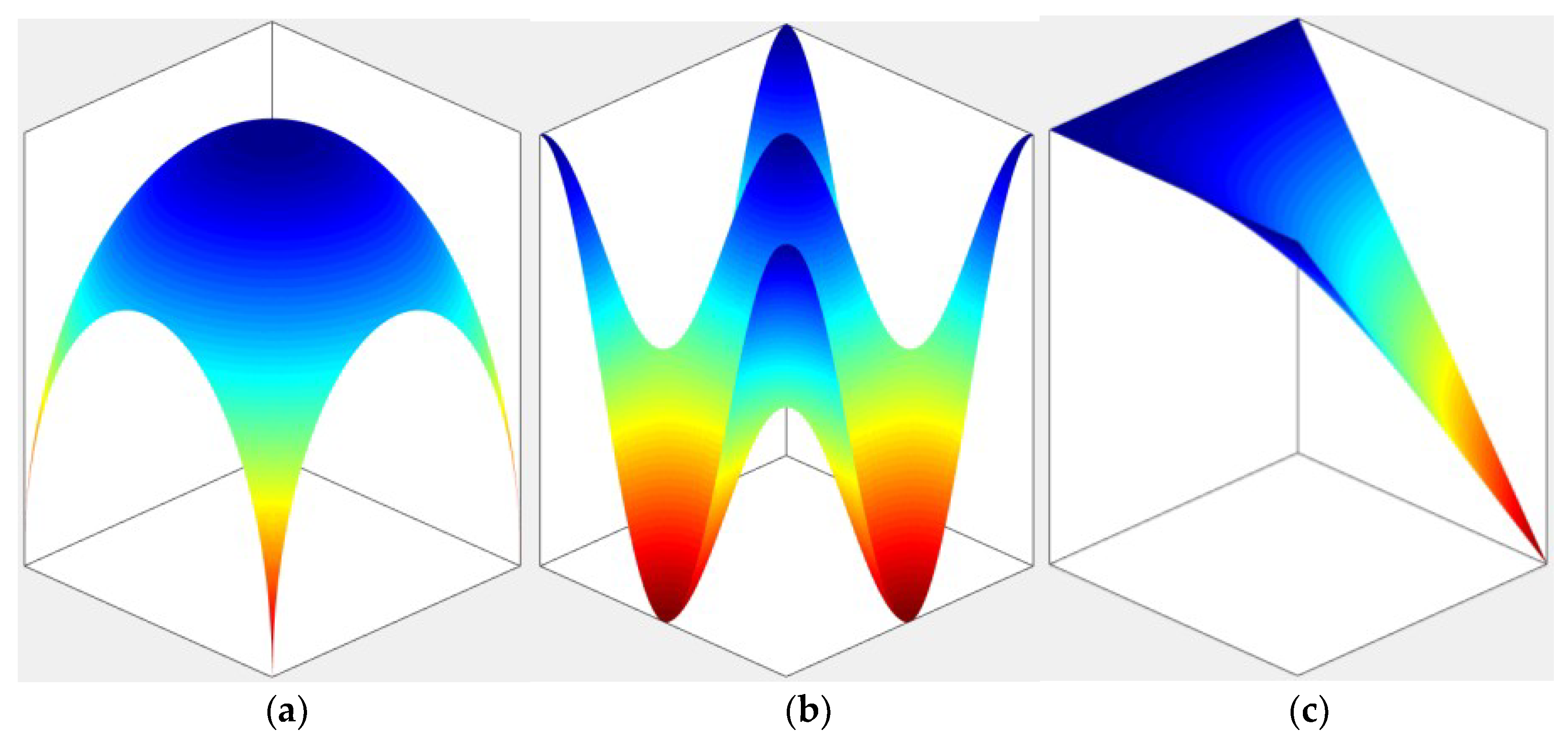
Test virtual objects: (a) Spherical surface; (b) Complex surface; (c) Simple surface.

Figure 15.
Initial depth map of the three models reconstructed using different evaluation windows of FSML.
Figure 15.
Initial depth map of the three models reconstructed using different evaluation windows of FSML.

Figure 16.
Initial depth map of the three models reconstructed using different evaluation windows of FTEN.
Figure 16.
Initial depth map of the three models reconstructed using different evaluation windows of FTEN.

Figure 17.
Initial depth map of the three models reconstructed using different evaluation windows of FGLV.
Figure 17.
Initial depth map of the three models reconstructed using different evaluation windows of FGLV.

Figure 18.
Test object and 3D model: (a) an actual entity of sprocket teeth; (b) 3D model of the sprocket teeth.
Figure 18.
Test object and 3D model: (a) an actual entity of sprocket teeth; (b) 3D model of the sprocket teeth.

Figure 19.
Image processing of the test: (a) the partial original images; (b) the partial pre-processed images; (c) the initial depth map; (d) the 3D recovery map.
Figure 19.
Image processing of the test: (a) the partial original images; (b) the partial pre-processed images; (c) the initial depth map; (d) the 3D recovery map.

Figure 20.
3D topographic recovery map reconstructed by FSML focus evaluation operator using different evaluation windows.
Figure 20.
3D topographic recovery map reconstructed by FSML focus evaluation operator using different evaluation windows.

Figure 21.
3D entities using different evaluation windows reconstructed by FSML focus evaluation operator.
Figure 21.
3D entities using different evaluation windows reconstructed by FSML focus evaluation operator.

Figure 22.
FSML focusing evaluation operator adopts different evaluation windows and original 3D entities of public part.
Figure 22.
FSML focusing evaluation operator adopts different evaluation windows and original 3D entities of public part.


Table 1.
Correlation and RMSE values of filtering effects of different filtering methods.
| Test Object | Vegetable | Ball | Human | ||||||
|---|---|---|---|---|---|---|---|---|---|
| Type | Noise Image | Median Filter | Normal Distribution Operator Filtering | Noise Image | Median Filter | Normal Distribution Operator Filtering | Noise Image | Median Filter | Normal Distribution Operator Filtering |
| Correlation | 0.9669 | 0.9977 | 0.9997 | 0.9440 | 0.9854 | 0.9956 | 0.9223 | 0.9842 | 0.9970 |
| RMSE | 58.9862 | 84.9033 | 104.6258 | 60.6358 | 74.1619 | 86.1075 | 46.8312 | 62.4062 | 79.2773 |
Table 2.
Evaluation result of the recovery effect of the three models reconstructed using different evaluation windows of FSML.
Table 2.
Evaluation result of the recovery effect of the three models reconstructed using different evaluation windows of FSML.
| Size | Cor | RMSE | ||||
|---|---|---|---|---|---|---|
| Spherical Surface | Complex Surface | Simple Surface | Spherical Surface | Complex Surface | Simple Surface | |
| 3 × 3 | 0.9823 | 0.9897 | 0.9972 | 0.0129 | 0.0323 | 0.0167 |
| 5 × 5 | 0.9899 | 0.9927 | 0.9978 | 0.0100 | 0.0302 | 0.0157 |
| 7 × 7 | 0.9942 | 0.9930 | 0.9979 | 0.0074 | 0.0286 | 0.0149 |
| Adaptive window | 0.9985 | 0.9936 | 0.9981 | 0.0036 | 0.0256 | 0.0121 |
Table 3.
Evaluation result of the recovery effect of the three models reconstructed using different evaluation windows of FTEN.
Table 3.
Evaluation result of the recovery effect of the three models reconstructed using different evaluation windows of FTEN.
| Size | Cor | RMSE | ||||
|---|---|---|---|---|---|---|
| Spherical Surface | Complex Surface | Simple Surface | Spherical Surface | Complex Surface | Simple Surface | |
| 3 × 3 | 0.9983 | 0.9947 | 0.9985 | 0.0075 | 0.0315 | 0.0165 |
| 5 × 5 | 0.9989 | 0.9954 | 0.9987 | 0.0058 | 0.0296 | 0.0156 |
| 7 × 7 | 0.9990 | 0.9954 | 0.9988 | 0.0045 | 0.0280 | 0.0148 |
| Adaptive window | 0.9994 | 0.9981 | 0.9991 | 0.0023 | 0.0209 | 0.0131 |
Table 4.
Evaluation result of the recovery effect of the three models reconstructed using different evaluation windows of FGLV.
Table 4.
Evaluation result of the recovery effect of the three models reconstructed using different evaluation windows of FGLV.
| Size | Cor | RMSE | ||||
|---|---|---|---|---|---|---|
| Spherical Surface | Complex Surface | Simple Surface | Spherical Surface | Complex Surface | Simple Surface | |
| 3 × 3 | 0.9940 | 0.9934 | 0.9803 | 0.0095 | 0.0337 | 0.0198 |
| 5 × 5 | 0.9990 | 0.9972 | 0.9859 | 0.0073 | 0.0312 | 0.0171 |
| 7 × 7 | 0.9990 | 0.9976 | 0.9933 | 0.0059 | 0.0295 | 0.0158 |
| Adaptive window | 0.9992 | 0.9981 | 0.9966 | 0.0028 | 0.0280 | 0.0128 |
Table 5.
Volume evaluation results of metal cones reconstructed by FSML at different evaluation windows/mm3.
Table 5.
Volume evaluation results of metal cones reconstructed by FSML at different evaluation windows/mm3.
| Evaluation Window | 3 × 3 | 5 × 5 | 7 × 7 | Adaptive Window |
|---|---|---|---|---|
| Vi | 32,021.26 | 32,037.06 | 32,089.74 | 32,056.08 |
| V0i | 31,468.01 | 31,488.91 | 31,550.28 | 31,833.45 |
| β | 95.09% | 95.17% | 95.38% | 97.23% |
© 2019 by the authors. Licensee MDPI, Basel, Switzerland. This article is an open access article distributed under the terms and conditions of the Creative Commons Attribution (CC BY) license (http://creativecommons.org/licenses/by/4.0/).
Share and Cite
MDPI and ACS Style
Ding, H.; Liu, Y.; Liu, J. Volumetric Tooth Wear Measurement of Scraper Conveyor Sprocket Using Shape from Focus-Based Method. Appl. Sci. 2019, 9, 1084. https://doi.org/10.3390/app9061084
AMA Style
Ding H, Liu Y, Liu J. Volumetric Tooth Wear Measurement of Scraper Conveyor Sprocket Using Shape from Focus-Based Method. Applied Sciences. 2019; 9(6):1084. https://doi.org/10.3390/app9061084
Chicago/Turabian StyleDing, Hua, Yinchuan Liu, and Jiancheng Liu. 2019. "Volumetric Tooth Wear Measurement of Scraper Conveyor Sprocket Using Shape from Focus-Based Method" Applied Sciences 9, no. 6: 1084. https://doi.org/10.3390/app9061084
Note that from the first issue of 2016, this journal uses article numbers instead of page numbers. See further details here.