A CNN Model for Human Parsing Based on Capacity Optimization

Department of Electronic and Information Engineering, The Hong Kong Polytechnic University, Hong Kong 999077, China
*
Author to whom correspondence should be addressed.
Appl. Sci. 2019, 9(7), 1330; https://doi.org/10.3390/app9071330
Submission received: 28 February 2019
/
Revised: 21 March 2019
/
Accepted: 21 March 2019
/
Published: 29 March 2019
(This article belongs to the Special Issue Intelligent Imaging and Analysis)
Abstract
:Although a state-of-the-art performance has been achieved in pixel-specific tasks, such as saliency prediction and depth estimation, convolutional neural networks (CNNs) still perform unsatisfactorily in human parsing where semantic information of detailed regions needs to be perceived under the influences of variations in viewpoints, poses, and occlusions. In this paper, we propose to improve the robustness of human parsing modules by introducing a depth-estimation module. A novel scheme is proposed for the integration of a depth-estimation module and a human-parsing module. The robustness of the overall model is improved with the automatically obtained depth labels. As another major concern, the computational efficiency is also discussed. Our proposed human parsing module with 24 layers can achieve a similar performance as the baseline CNN model with over 100 layers. The number of parameters in the overall model is less than that in the baseline model. Furthermore, we propose to reduce the computational burden by replacing a conventional CNN layer with a stack of simplified sub-layers to further reduce the overall number of trainable parameters. Experimental results show that the integration of two modules contributes to the improvement of human parsing without additional human labeling. The proposed model outperforms the benchmark solutions and the capacity of our model is better matched to the complexity of the task.
1. Introduction
Semantic segmentation and human parsing are critical tasks in visually describing humans under various scenes. Deep Convolutional Neural Networks (CNNs) have brought significant improvements to human parsing tasks [1,2,3] thanks to the availability of an increased amount of training data. Existing works in this field include Path Aggregation (PA) [4], Large Kernel Matters (LKM) [5], Mask RCNN (MRCNN) [6], holistic models for human parsing [7], and joint pose estimation and part segmentation [8] with spatial pyramid pooling [9]. Moreover, human parsing aligns well with other tasks such as group behavior analysis [10], person re-identification [11], e-commerce [12], image editing [13], video surveillance [14], autonomous driving [3], and virtual reality [15].
However, the performance of existing human parsing methods is still far from robust due to the heavy reliance on the limited training data. In real-world scenarios, one image is very likely to contain multiple people with various human interactions, poses, and occlusion. However, very few of the scenarios can be included in common datasets. For instance, the Pascal Person Part Dataset [7] contains annotations of less than 10 classes and no more than 4,000 images for training and validation, which is far from enough to train complex CNNs [16,17] with over 100 layers. What is worse, is that data augmentation is challenging because labeling an image pixel-by-pixel takes 239.7 s on average [18].
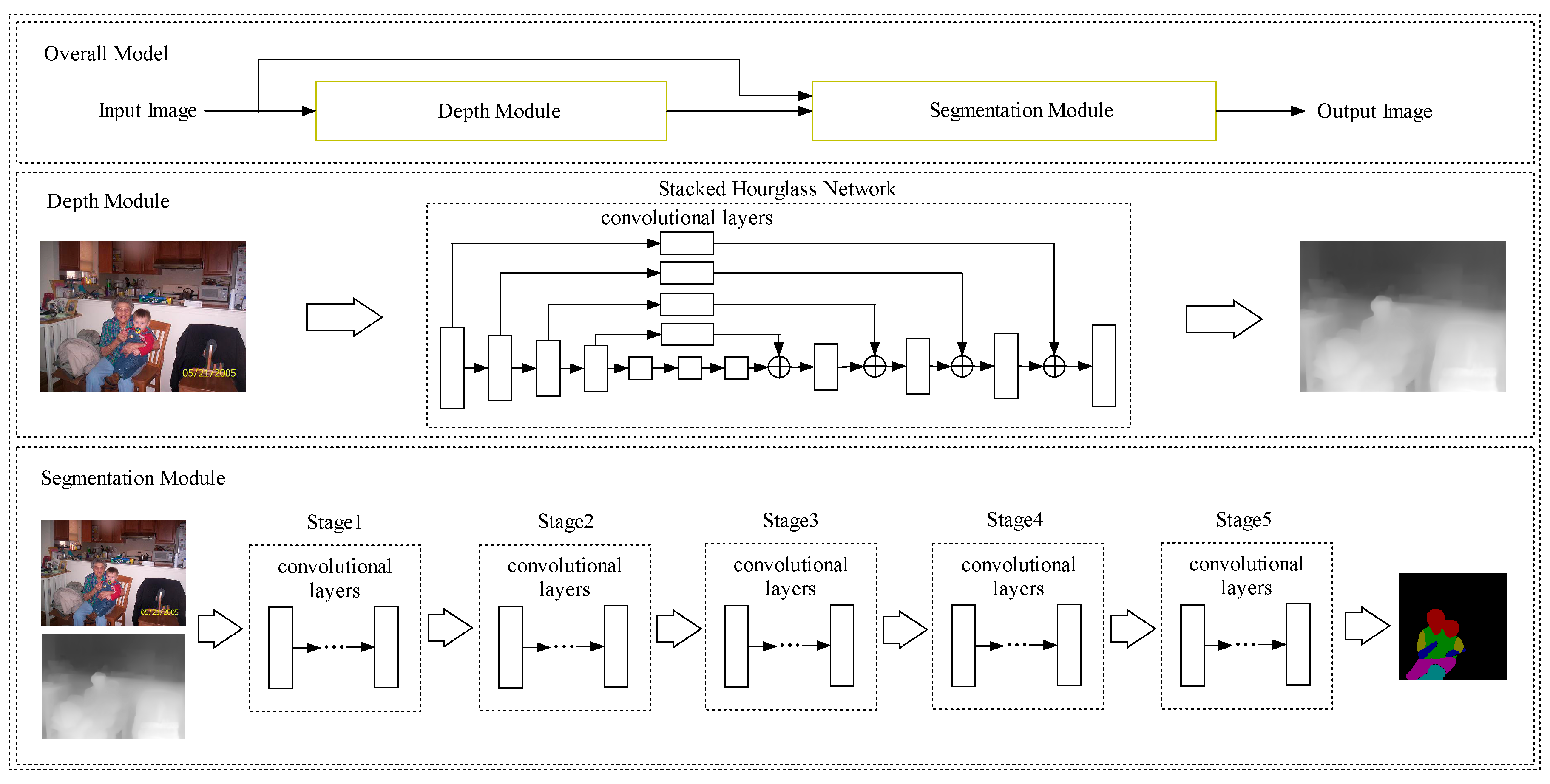
To reduce the cost in labelling, image-level annotations and bounding boxes have been adopted by weakly supervised methods to improve segmentation [19,20,21]. Additionally, scribbles and points have been introduced in [18,22] as auxiliary supervision. Unlike most weakly supervised methods, depth information is utilized in this paper as guidance to help distinguish foregrounds from backgrounds and use the limited capacity of a CNN model more on foreground areas. A module for depth estimation was trained firstly, then the concatenation of the depth predictions and RGB images composed the input to the segmentation module during both training and testing processes. For simplicity, we used the Depth-Module (DM) and Segmentation-Module (SM) to represent the two modules. The depth annotations from RGB image pairs with overlapping viewpoints could be obtained automatically [23] with multi-view stereo (MVS). The two modules composed the Overall Model (OM).
The advantage of integrating a Depth-Model with Segmentation-Module comes in two ways. Firstly, the training data for depth estimation can cover the variations which seldomly appear in the training data for human parsing. Robustness is improved in this way. Secondly, depth estimation and segmentation are closely correlated. The former assigns continuous depth values to pixels while the latter assigns discrete categorical labels to pixels. The predicted depth maps facilitate hierarchical descriptions of images which are helpful for segmentation. The learning process is divided into two stages: (1) To train the DM on the large-scale MegaDepth Dataset [24] collected from Internet photos. (2) Both the training and testing of SM were based on the predictions from the DM and original RGB images [2,7]. The strategy introduced in Section 3.3 was applied. As is shown in Figure 1, DM helped to focus the SM’s limited capacity on the qualified regions and boost the performance of segmentation. Each input image of the SM had four channels, RGB and the depth prediction from DM.
Existing works on optimizing the capacity of CNNs are divided into three categories. The first type of work [27,28] explores the sparseness of feature representations within a CNN and keeps only branches which are useful to tasks. The second type of work [29] makes use of the favorable properties of a shallow network and improves the performance of the CNN based on novel training strategies. The third type of work [30] maximizes the representational power of a CNN by maximizing the number of inter-connections between the features in different levels. Although the existing methods have improved computational efficiency, none of them has explored the relationship between depth and accuracy. This paper proposes a way to match the representational power and capacity of a CNN to a task by adjusting the depth and width of the CNN and training the CNN with a novel scheme. Both quantitative and qualitative experiments are conducted on the LIP Dataset [26] and the Pascal Person Part Dataset [7] to show that the proposed model conducts human parsing in a more effective and time-efficient manner.
In summary, the contributions of this paper are in three aspects: (1) A model for human parsing is proposed with integrated DM and SM modules. Moreover, a novel scheme is proposed for training the modules. The DM is trained on a large amount of automatically labeled images and provides information which is complementary to the features in the SM. As a result, the OM outperforms the SM only, especially at the boundaries. (2) A new algorithm is proposed to train the SM with 24 layers, achieving a similar performance as the baseline model with over 100 layers trained on the currently largest dataset for human parsing. (3) The influences of depth and width on capacity are studied. Two methods are proposed to build a SM which is deeper with performance improvement but uses less parameters. As a result, the performance-complexity ratio is improved and the capacity of the CNN model is better utilized.
The rest of the paper is organized as follows. Section 2 introduces related work. Section 3 discusses the details of our proposed model and the method for adjusting the CNN’s capacity. Section 4 shows the details of implementation as well as experimental results. Concluding remarks are drawn in Section 5.
2. Related Work
Human Parsing Approaches. Human parsing has become an active research topic in the last few years [7,9,21,26,31,32,33]. The JPPNet [8] and the Nested Adversarial Network [34] represent the current state-of-the-art methods. The improvements in the methods, such as those in Reference [8,23], over traditional methods [9] are achieved by combining pose estimation with semantic part segmentation. The estimated poses provide the shape prior, which is necessary for segmentation. Similarly, the authors of Reference [35] proposed to integrate parsing with optical flow estimation. The authors of Reference [36] incorporated a self-supervised joint loss to ensure the consistency between parsing and pose. However, the guidance from poses cannot improve borders. As a result, it is still quite difficult to delineate the boundaries. In our proposed method, it is shown that depth information can improve the classification of pixels near boundaries. Other work, such as Reference [34], proposed to integrate three sub-nets which perform semantic saliency prediction, instance-agnostic parsing, and instance-aware clustering, respectively. The authors of Reference [37] proposed a framework integrating a human detector and a category-level segmentation module. However, both methods involve multiple stages. The outputs from earlier stages compose the only inputs to later stages and misleading outputs from the earlier stages disable the later stages. In our proposed method, the input to the SM composes not only the output from the DM, but also the original RGB images. The SM is less dependent on the DM and can function even when the DM fails.
Weakly Supervised Methods. To tackle the lack in training data, three types of research works have been conducted. The first type involves learning based on bounding boxes, scribbles, image tags or mixing multiple types of annotations. The labels in the form of bounding boxes and scribbles indicate the locations and sizes of objects. The BoxSup proposed in [20] and DeepCut proposed in [38] trained the segmentation model based on iterating between bounding box generation and training the CNN. The 3D U-Net proposed in Reference [39] performed volumetric segmentation with a semi-automated setup or a fully-automated setup. The multi-task learning proposed in Reference [40] adopted image-level and point-level supervision. Image-level supervision shows whether certain objects are present in an image. Point-level supervision indicates the locations and rough boundaries of objects. Bounding boxes and scribbles were mixed in Reference [21,41] to facilitate better training. However, the methods cannot deal with images containing multiple people or those with complex backgrounds.
The second type of work focuses on predicting the weights of a model in a target task, such as image classification using the weights from a source task, such as natural language descriptions or few-shot examples [42,43,44]. Among vision tasks, the authors of Reference [45] proposed to transform the weights in a detection model to those in a segmentation model. Similarly, the LSDA (Large Scale Detection Through Adaptation) proposed in Reference [46] introduced a way to transform a classification model to a detection model. The rationality lies in the fact that more training data are available in source domains. However, the transformation of weights is based on a parameterized function which is learned on the limited annotations from a target domain. The taskonomy proposed in Reference [47] re-used the supervision among related tasks. It trains higher-order transfer functions to map the feature representations from a source task to a target task. However, different types of annotations need to be present on the same set of images. The requirements on annotations limits the scale of training data. Different from the above-mentioned methods, our proposed human parsing model utilizes depth information without learning a parameterized function. The DM can be trained on large datasets with only depth annotations and provide robust predictions on images with multiple people or those with complex backgrounds. The SM benefits from the complementary features provided by the DM and the segmentation performance is improved.
Capacity Optimization. The definition of capacity is introduced in Reference [48]. The term capacity tends to relate to volumes, quantities or memorization. It measures how complex a function a neural network can model. Existing work on capacity optimization includes pruning feature representations [49,50,51], exploring favorable properties of a shallow network [29], and maximizing the expressive power of a fixed-size network [16,30]. The first type of work focuses on pruning convolutional kernels to obtain the most compressed sets of feature representations required for a task. However, most of the related methods improved the processing speed at the cost of accuracy. The second type of method replaces the end-to-end training scheme by a sequentially training scheme. Accuracy is improved without increasing depth. However, the depth of a CNN is not yet well matched to a task. Our proposed training scheme outperforms the scheme in Reference [29], as will be shown in Section 4.3. The third type of work [30] tried to improve the performance-complexity ratio, but the added connections significantly reduced the efficiency in memory accessing. In our proposed scheme, the depth of a CNN is better matched to the complexity of a human parsing task. Moreover, a deeper but more efficient module is built to optimize the capacity of a CNN without dropping in accuracy. Experimental results will demonstrate the superiority of our proposed methods.
3. Methodology
Our proposed model is shown in Figure 1. The complementary nature of the SM and DM is explored. Besides color, the depth prediction provided by the DM facilitates an extra way to understand images to improve segmentation. To be more specific, nearby regions belonging to different instances are predicted to share the same label by the SM because of similar colors and textures. However, the regions can be differentiated from each other by the DM because of the difference in their depth values.
As is shown in Figure 2, the results of using the SM only for segmentation and those of integrating the SM with the DM are compared. It is shown in the first row that the heads of different identities cannot be distinguished because of the similarity in colors. However, the depth predictions help to differentiate the instances. In the second row, foreground instances share the same color as backgrounds. The depth predictions help to segment out foreground instances. Similarly, the lower arms in the third row can hardly be distinguished from the background with color information only. Successful segmentation results from depth predictions.
3.1. Depth Module
Similar to other network models which output the same resolution as the inputs [37,52], the DM is also trained end-to-end. It processes and passes information across multiple scales. The design of the DM is based on the stacked hour-glass network proposed in Reference [25,53]. The symmetric structure consists of convolutions, pooling layers which are followed by up-sampling layers and convolutions. The detailed structure was discussed in Reference [54].
The loss function for training the network is the weighted sum of three terms. The first term denotes the mean square error of predicted depth values.
where denotes the difference between the prediction at the -th pixel and the corresponding ground truth depth value. denotes the number of pixels. The training images are from the large-scale MegaDepth dataset [24]. is invariant to the shifts on the mean values of images. The second term takes into consideration the gradients on the difference map:
This term improves the performance on sharp discontinuities and makes depth predictions smoother. The third term enforces the ordinal depth relations between foreground super-pixels and background super-pixels:
pairs of points are sampled from the depth predictions and ground truth depth maps. denotes the -th point sampled from the largest foreground super-pixel while denotes the -th point sampled from the surrounding background super-pixels. denotes the depth at point and the depth at point . The weight of in the loss function is set to 0.5 while the weight of is set to 0.1. The existence of term Equation (3) enforces the predicted depth values of neighboring instances to be different and ordered. The overall lost function is defined as
3.2. Segmentation Module
In this section, an SM with 24 layers is introduced, which is compared with the baseline model Deeplab-V2 [9] on the segmentation task.
3.3. Strategy of Combining DM with SM
Solely integrating the predictions from the DM with RGB images during training and testing the SM only brings slight improvements. However, better strategies can be adopted to fully explore the complementary nature of color and depth information to contribute more to performance improvement. In this section, we propose a strategy to better utilize depth information. The strategy is divided into two steps. An example is shown in Figure 4.
In the first step, the DM is trained and used to augment the training data and test data of the SM. OM segments out foreground objects as one class. To reduce false negatives, dilation is conducted on the masks produced by the OM. In the second step, the regions which are predicted by Step 1 as foregrounds are kept unchanged, with remaining parts set to zero. The images produced by Step 2 are then used for re-training and testing SM. Table 1 compares the performance of three cases: Only using the SM, direct training and testing of the SM based on the predictions from the DM and applying the strategy in this section to combine DM with the SM.
3.4. Capacity Optimization of SM
Each input image is mapped by a CNN from the image space to the feature space , a CNN learns the low-dimensional structures of data and represents them using a parametric polyhedral manifold which is then partitioned into pieces [60]. The more pieces there are, the higher the representation capability of the CNN becomes. For a ReLU deep neural network, each neuron functions as a hyperplane and partitions the input manifold into multiple polyhedra. As a result, the number of pieces is decided by the number of ReLU operations. The bound of the encoding or representation capability of a ReLU DNN is measured by Rectified Linear Complexity (RL Complexity) . For a neural network with hidden layers of widths , the upper bound of RL Complexity is given by
where
Only when the RL complexity of a neural network is no less than that of the manifold can the data be encoded by the neural network. It can be inferred from Equations (5) and (6) that the depth of neural network contributes much more significantly to the capacity of a neural network than width. As a result, we have made the CNN in Figure 3a deeper than the backbone [55]. The contribution to performance improvement from additional depth will be shown in Section 4.2 and Section 4.4.
Moreover, we have also developed a scheme for training the CNN in Figure 3a, as is shown in Algorithm 1. The training is conducted layer by layer because it was discussed in Reference [29] that a CNN with a fixed number of layers can perform better if it is built sequentially layer by layer instead of trained end-to-end.
| Algorithm 1: Scheme of training SM | |
| Step 1 | Train the backbone network [55] without layers conv3, conv6, conv10, conv14, conv18 until convergence. |
| Step 2 | Add layer conv18 which is initialized with Gaussian weight matrices. |
| Step 3 | Use the pre-trained layers conv1-conv17 to extract the feature vectors from images and use the feature vectors as the input to train conv18. |
| Step 4 | Freeze the weights in all layers in Stage 6 and Stage 7 and train conv18 until convergence. |
| Step 5 | Re-train SM until convergence with all layers un-frozen. |
| Step 6 | Add layer conv14, conv10, conv6, conv3 and go through the same operations from Step 2 to Step 5. |
Different from Reference [29] which only trained the added layer each time, for each added layer in Algorithm 1, the network is trained for two times. In the first time the added layer only is trained while in the second time, the overall network is trained. As will be shown in Section 4.3 the strategy of our adding layers has an advantage over both adding all layers together at once and applying the method in Reference [29]. Moreover, the involvement of the five additional layers has brought significant improvements in accuracy over the backbone network, as will be shown in Section 4.2.
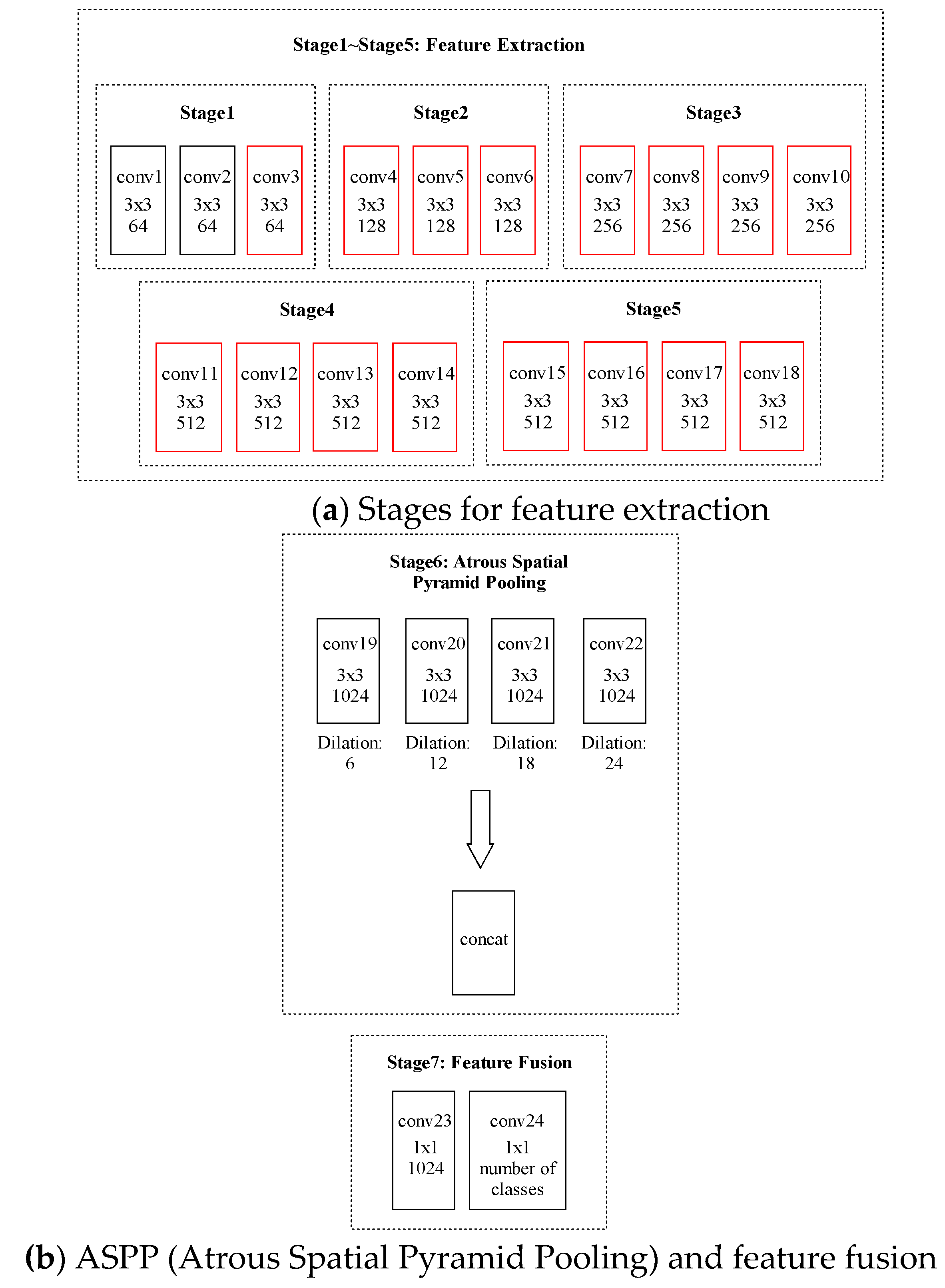
Different from traditional segmentation models, the feature representations at Stage 6 which correspond to 4 point-of-views are concatenated and fused by the 1 × 1 convolutions at Stage 7, as compared to the direct summation in Reference [8]. Feature fusion offers a much more flexible scheme of combining the features from different point-of-views. The network can learn to add up the features or combine the features in more complex ways.
Besides improving depth which leads to the increase in computational complexity, we also propose to exchange width for depth to obtain further improvements in accuracy while reducing the number of parameters. Two methods have been proposed to reduce the complexity of convolutional layers by replacing one conventional convolutional layer with a stack of simplified layers. The overall complexity of stacked simplified layers is less than that of one original convolutional layer. The mechanism is shown in Figure 5. Figure 5b shows our first proposed way of exchanging width for depth. In one conventional layer, independent 3 × 3 convolutional kernels function on channels to obtain one output channel. In one simplified sub-layer, () kernels function on each of the input channels and the intermediate representation has output channels which are processed by 1 × 1 convolutions. is the number of sub-layers which are stacked to replace one conventional layer. Even if one sub-layer is less expressive than one conventional layer with the same and , the stack of sub-layers achieves a higher expressive power than one conventional layer without increasing the overall number of parameters for proper choices of and . In Figure 5c, the second way of exchanging width for depth is introduced. Each conventional layer is replaced by two sub-layers. The difference lies in that Figure 5b uses 4 sub-layers to replace one conventional layer, while Figure 5c uses two sub-layers.
The structures introduced in Figure 5b and c will be used to simplify conv17 and conv18 shown in Figure 3. As will be shown in the experiments, accuracy is kept almost the same with the overall computational complexity reduced. Deeplab-V2 [9] and joint pose estimation and part segmentation [8] which is based on Resnet-101 [9] are also trained on the segmentation datasets for comparison.
The initialization of weights in Figure 5b was discussed in Reference [61] and the initializations of weights in Figure 5c is based on minimizing the reconstruction error:
where denotes the weights matrix in one layer shown in Figure 5a with size , with denoting the -th row of . denotes the weights in Sub-layer 1 with being the -th row of the matrix. denotes the weights in Sub-layer 2 with being the -th entry of the matrix.
3.5. Domain Randomization
To reduce the generalization error, it is necessary to bridge the gap between the source domain (training data) and the target domain (test data). Some methods have been proposed to discuss the problem [62]. However, these methods mainly focus on other tasks, such as object detection [62], in which all types of simulated variability at training time are utilized, including positions, textures, orientations, field-of-views, and lightening conditions. Too many variations may result in a low convergence rate.
The LIP dataset includes the variations in poses and lightening conditions in the training set. As a result, we are only concerned with the variations in backgrounds which contribute to the divergence between domains. We propose to crop the predicted backgrounds from test images, which are then used to fill the background regions in training images. In this way, an augmented training dataset is produced to help the SM develop more generalizable representations. The detailed scheme is introduced in Algorithm 2.
| Algorithm 2: Scheme of domain randomization | |
| Step 1 | Train SM until convergence and use it to segment out the background regions of test images. |
| Step 2 | For each training image, find the image from test set with the most similar aspect ratio. Resize the test image to be with the same size as the training image. |
| Step 3 | Crop the background regions from the test image and replace the background regions on the training image with those from the test image. |
| Step 4 | Re-train SM and return to Step 1. (Two iterations are adopted.) |
Figure 6 shows two examples of domain randomization. The backgrounds in training images are replaced by those in test images.
4. Results
4.1. Datasets and Implementation Details
The two modules in our proposed model were trained on two datasets. The DM was trained on the MegaDepth Dataset [24] which involves 130K images from 200 different landmarks. The depth information in images with over-lapping viewpoints is automatically obtained with SFM (Structure from Motion) and MVS (Multi-View Stereo). The SM was trained on the images from the PASCAL VOC 2010 Person Part Dataset for body part segmentation [2,63]. The Person Part Dataset includes annotations on 3,533 images where 1,716 images are used for training while the other 1,817 images are for testing. The ground truth labels are in the form of segmentation masks. There are six annotated semantic types, that is, head, torso, upper arm, lower arm, upper leg, lower leg, and background. To evaluate on larger datasets and to demonstrate the improvement on capacity, the SM was also trained on the LIP (Look into Person) Dataset [26] with 30,462 images for training, 10,000 images for validation and 10,000 test images. There are 19 annotated semantic types, that is, face, upper clothes, hair, right arm, pants, left arm, right shoe, left shoe, hat, coat, right leg, left leg, glove, socks, sunglasses, dress, skirt, jumpsuits, scarf. The capacity of the SM was optimized using the two methods shown in Figure 5.
4.2. Integration of the Two Modules
As is shown in Figure 1, the DM is used to preprocess an image and predict depth masks. The predicted masks are concatenated with corresponding input RGB images to produce the input of the SM during both training and testing. The experiments were conducted to show that the combination of color and depth information during training and inference improves the performance of human parsing. The metric for evaluating the performance of human parsing is mean Intersection Over Union (mIOU) which is proposed in [7]. mIOU is computed by dividing the number of true positive samples by the summation of true positive, false negative, and false positive samples:
where is the number of pixels of class which are predicted to class , and is the total number of pixels belonging to class . The metric takes into account both false positives and false negatives. For the Pascal VOC 2010 Person Part Dataset, mIOU is computed for each of the seven classes and averaged. For instance, the mIOU of head is obtained by regarding head as the foreground and other six types as the backgrounds. Table 1 shows the results on the test set.
For the LIP Dataset, mIOU is computed in the same way and the experimental results are shown in Table 2.
By comparing the last three rows in Table 1 and the last two rows in Table 2, it can be inferred that the integration of the DM and the SM outperforms the SM on both large and small datasets. Table 1 shows that the contribution is mainly attributed to the scheme proposed in III-C, which fully explores the complementary nature of the DM and the SM.
Moreover, it is discussed in Section 3.2 that the backbone of the SM is Deep Lab-V2 (VGG-16) [9] with 18 layers. Figure 7 shows the changes in accuracy upon increasing the depth of SM from 18 to 24. With the six added layers, the SM not only outperforms the backbone, but also performs as well as the baseline model with over 100 layers which is shown in the second row in Table 2. Note that the number of parameters in the OM is less than that in the baseline model [9]. More importantly, LIP is the currently largest dataset for human parsing and the number of parameters in SM is much less than that in the baseline model. The improvement demonstrates that by adjusting the depth of a CNN model, its capacity is better matched to a task than Reference [8,9].
4.3. The Advantage of Layer-Wise Training
As is demonstrated by the second and third rows in Table 2, the SM can perform as well as a model that is much more complex. The advantage results from the layer-wise training scheme which is proposed in Section 3.4 and shown in Algorithm 1. To demonstrate the advantage of Algorithm 1 over adding all the layers to the backbone at once, we compare the performance of the SMs trained with the two schemes and show the results in Table 3. In the scheme where all the layers are added at once and the SM was trained for one time, the number of iterations during training is 600,000. In the scheme proposed in Algorithm 1, the SM was trained for 100,000 iterations upon the addition of each layer. The overall time cost during training is the same. The performance is evaluated on the LIP Dataset.
It can be inferred from Table 3, that layer-wise training significantly outperforms direct training all layers at once. Different from the layer-wise training in Reference [29], we firstly train each added layer while keeping other layers fixed for 50,000 iterations and then re-training all layers for another 50,000 iterations. Compared with training each added layer for 100,000 iterations, Algorithm 1 performs better, as is shown by the last two rows in Table 3.
4.4. The Exchange Between Width and Depth for Capacity Optimization
We have also tried to replace traditional convolutional layers with the stacking of simplified convolutional layers shown in Figure 5b,c. The in Figure 5b is chosen to be 3 and the number of sub-layers is selected to be 4. We have replaced conv18 in Figure 3 with the stacked simplified layers. Upon replacing the layer, the SM is re-trained for 100,000 iterations. The changes in performance and the drop in computational burden is shown in Table 4. The performance is evaluated on the LIP dataset.
The initializations of the weights in the layers in Figure 5b,c are discussed in Section 3.4.
4.5. Domain Randomization
We augmented the training data with domain randomization where the backgrounds in training images were replaced by the counterparts in test images. In the implementation of Algorithm 2, we cropped the backgrounds from two test images to replace the background of each training image. As a result, the augmented dataset includes 60,924 images.
It can be inferred from Table 5 that iterative domain randomization improves the generalization of the SM.
4.6. Examples of Segmentation Results
Besides objective results, some results are shown in Figure 8 and Figure 9 to show the advantages of integrating the DM with the SM which can be judged subjectively. A comparison between the SM and the OM is made on multiple cases, including samples with complex gestures in identities, images with occlusions, and those suffering from darkness.
5. Discussion
In this paper, depth information is combined with color using a novel strategy. The performance of human parsing is significantly improved. Moreover, depth information is obtained by a module which is trained on automatically acquired labels, thus saving human labor cost. Secondly, the SM with 24 layers, which is trained using the scheme in Algorithm 1 achieves a similar performance as the baseline model with over 100 layers on the currently largest dataset for human parsing. The number of parameters in the OM is less than that in the baseline model. Thirdly, two methods have been proposed to optimize the capacity of the SM by increasing depth while reducing parameters, achieving a more efficient solution with a better performance. Both quantitative and subjective results have shown the effectiveness of our proposed methods.
Author Contributions
Conceptualization, Y.J. and Z.C.; methodology, Y.J.; software, Y.J.; writing—original draft preparation, Y.J.; writing—review and editing, Y.J. and Z.C.; supervision, Z.C.
Acknowledgments
The work described in this paper was partially supported by a Natural Science Foundation of China (NSFC) grant (Project Code: 61473243). Yalong Jiang would like to acknowledge the financial support from The Hong Kong Polytechnic University for his PhD study.
Conflicts of Interest
The authors declare no conflict of interest.
References
- Lin, T.; Maire, M.; Belongie, S.; Hays, J. Microsoft coco: Common objects in context. In Proceedings of the European Conference on Computer Vision, Zurich, Switzerland, 6–12 September 2014. [Google Scholar]
- Everingham, M.; Eslami, S.A.; Van Gool, L. The pascal visual object classes challenge a retrospective. Int. J. Comput. Vis. 2015, 111, 98–136. [Google Scholar] [CrossRef]
- Cordts, M.; Omran, M.; Ramos, S.; Rehfeld, T. The cityscapes dataset for semantic urban scene understanding. In Proceedings of the IEEE Conference on Computer Vision and Pattern Recognition, Las Vegas, NV, USA, 26 June–1 July 2016. [Google Scholar]
- Liu, S.; Qi, L.; Qin, H.; Shi, J.; Jia, J. Path aggregation network for instance segmentation. arXiv, 2018; arXiv:1803.01534. [Google Scholar]
- Peng, C.; Zhang, X.; Yu, G.; Luo, G.; Sun, J. Large Kernel Matters—Improve Semantic Segmentation by Global Convolutional Network. arXiv, 2017; arXiv:1703.02719. [Google Scholar]
- He, K.; Gkioxari, G.; Dollár, P.; Girshick, R. Mask r-cnn. arXiv, 2017; arXiv:1703.06870. [Google Scholar]
- Chen, X.; Mottaghi, R.; Liu, X.; Fidler, S. Detect what you can: Detecting and representing objects using holistic models and body parts. In Proceedings of the IEEE Conference on Computer Vision and Pattern Recognition (CVPR), Columbus, OH, USA, 24–27 June 2014. [Google Scholar]
- Xia, F.; Wang, P.; Chen, X.; Yuille, A. Joint Multi-person Pose Estimation and Semantic Part Segmentation. In Proceedings of the IEEE Conference on Computer Vision and Pattern Recognition, Honolulu, HI, USA, 22–25 July 2017. [Google Scholar]
- Chen, L.C.; Papandreou, G.; Kokkinos, I. Deeplab: Semantic image segmentation with deep convolutional nets, atrous convolution, and fully connected crfs. IEEE Trans. Pattern Anal. Mach. Intell. 2018, 40, 834–848. [Google Scholar] [CrossRef] [PubMed]
- Gan, C.; Lin, M.; Yang, Y.; de Melo, G. Concepts not alone: Exploring pairwise relationships for zero-shot video activity recognition. In Proceedings of the AAAI 2016, Phoenix, AZ, USA, 12–17 February 2016. [Google Scholar]
- Zhao, R.; Ouyang, W.; Wang, X. Unsupervised salience learning for person re-identification. In Proceedings of the IEEE Conference on Computer Vision and Pattern Recognition, Portland, OR, USA, 25–27 June 2013. [Google Scholar]
- Turban, E.; King, D.; Lee, J.; Viehland, D. Electronic Commerce: A Managerial Perspective 2002; Prentice Hall: Upper Saddle River, NJ, USA, 2002; Volume 2. [Google Scholar]
- Xu, N.; Price, B.; Cohen, S.; Yang, J.; Huang, T. Deep interactive object selection. In Proceedings of the IEEE Conference on Computer Vision and Pattern Recognition, Las Vega, NV, USA, 26 June–1 July 2016. [Google Scholar]
- Collins, R.; Lipton, A.; Kanade, T. A System for Video Surveillance and Monitoring; VSAM Final Report; Robotics Institute, Carnegie Mellon University: Pittsburgh, PA, USA, 2000; Volume 2, pp. 1–68. [Google Scholar]
- Lin, J.; Guo, X.; Shao, J.; Jiang, C.; Zhu, Y. A virtual reality platform for dynamic human-scene interaction. In Proceedings of the SIGGRAPH, San Jose, CA, USA, 24–28 July 2016. [Google Scholar]
- He, K.; Zhang, X.; Ren, S.; Sun, J. Deep residual learning for image recognition. Comput. Vis. Pattern Recognit. arXiv, 2016; arXiv:1512.03385. [Google Scholar]
- Szegedy, C.; Ioffe, S.; Vanhoucke, V.; Alemi, A. Inception-v4, inception-resnet and the impact of residual connections on learning. In Proceedings of the AAAI, San Francisco, CA, USA, 4–9 February 2017. [Google Scholar]
- Bearman, A.; Russakovsky, O.; Ferrari, V.; Li, F. What’s the point: Semantic segmentation with point supervision. In Proceedings of the European Conference on Computer Vision, Amsterdam, The Netherlands, 8–16 October 2016. [Google Scholar]
- Pathak, D.; Krahenbuhl, P.; Darrell, T. Constrained convolutional neural networks for weakly supervised segmentation. In Proceedings of the IEEE International Conference on Computer Vision, Santiago, Chile, 11–18 December 2015. [Google Scholar]
- Dai, J.; He, K.; Sun, J. Boxsup: Exploiting bounding boxes to supervise convolutional networks for semantic segmentation. In Proceedings of the IEEE International Conference on Computer Vision, Santiago, Chile, 11–18 December 2015. [Google Scholar]
- Papandreou, G.; Chen, L.; Murphy, K.; Yuille, A. Weakly-and semi-supervised learning of a DCNN for semantic image segmentation. arXiv, 2015; arXiv:1502.02734. [Google Scholar]
- Sun, J.; Lin, D.; Dai, J.; Jia, J.; He, K. Scribblesup: Scribble-supervised convolutional networks for semantic segmentation. In Proceedings of the IEEE Conference on Computer Vision and Pattern Recognition, Las Vegas, NV, USA, 26 June–1 July 2016. [Google Scholar]
- Snavely, N.; Seitz, S.; Szeliski, R. Photo tourism: Exploring photo collections in 3D. ACM Trans. Graph. 2006, 25, 835–846. [Google Scholar] [CrossRef]
- Snavely, N.; Li, Z. MegaDepth: Learning Single-View Depth Prediction from Internet Photos. In Proceedings of the IEEE Conference on Computer Vision and Pattern Recognition, Salt Lake City, UT, USA, 19–21 June 2018. [Google Scholar]
- Newell, A.; Yang, K.; Deng, J. Stacked hourglass networks for human pose estimation. In Proceedings of the European Conference on Computer Vision, Amsterdam, The Netherlands, 8–16 October 2016. [Google Scholar]
- Liang, X.; Gong, K.; Shen, X.; Lin, L. Look into Person: Joint Body Parsing & Pose Estimation Network and A New Benchmark. arXiv, 2018; arXiv:1804.01984v1. [Google Scholar]
- Ierusalem, A. Catastrophic Importance of Catastrophic Forgetting. arXiv, 2018; arXiv:1808.07049. [Google Scholar]
- He, Y.; Lin, J.; Liu, Z.; Wang, H. Amc: Automl for model compression and acceleration on mobile devices. In Proceedings of the European Conference on Computer Vision (ECCV), Munich, Germany, 8–14 September 2018. [Google Scholar]
- Shallow learning for deep networks. Int. Conf. Learn. Represent. 2019. Under review.
- Huang, G.; Liu, Z.; Van Der Maaten, L. Densely Connected Convolutional Networks. In Proceedings of the IEEE Conference on Computer Vision and Pattern Recognition, Honolulu, HI, USA, 22–25 July 2017. [Google Scholar]
- Ronneberger, O.; Fischer, P.; Brox, T. U-net: Convolutional networks for biomedical image segmentation. In Proceedings of the International Conference on Medical Image Computing and Computer-Assisted Intervention, Munich, Germany, 5–9 October 2015. [Google Scholar]
- Pohlen, T.; Hermans, A.; Mathias, M.; Leibe, B. Full-resolution residual networks for semantic segmentation in street scenes. arXiv, 2017; arXiv:1611.08323. [Google Scholar]
- Chen, L.; George, P.; Florian, S.; Hartwig, A. Rethinking atrous convolution for semantic image segmentation. arXiv, 2017; arXiv:1706.05587. [Google Scholar]
- Zhao, J.; Li, J.; Cheng, Y.; Zhou, L.; Sim, T. Understanding Humans in Crowded Scenes: Deep Nested Adversarial Learning and A New Benchmark for Multi-Human Parsing. arXiv, 2018; arXiv:1804.03287. [Google Scholar]
- Liu, S.; Wang, C.; Qian, R.; Yu, H.; Bao, R. Surveillance video parsing with single frame supervision. In Proceedings of the IEEE Conference on Computer Vision and Pattern Recognition, Honolulu, HI, USA, 22–25 July 2017. [Google Scholar]
- Zhao, J.; Li, J.; Nie, X.; Zhao, F.; Chen, Y.; Wang, Z.; Feng, J.; Yan, S. Self-supervised neural aggregation networks for human parsing. In Proceedings of the IEEE Conference on Computer Vision and Pattern Recognition, Honolulu, HI, USA, 22–25 July 2017. [Google Scholar]
- Li, Q.; Arnab, A.; Torr, P. Holistic, instance-level human parsing. arXiv, 2017; arXiv:1709.03612. [Google Scholar]
- Oktay, O.; Kamnitsas, K.; Passerat-Palmbach, J. Deepcut: Object segmentation from bounding box annotations using convolutional neural networks. IEEE Trans. Med. Imag. 2017, 36, 674–683. [Google Scholar]
- Çiçek, Ö.; Abdulkadir, A.; Lienkamp, S.; Brox, T. 3D U-Net: Learning dense volumetric segmentation from sparse annotation. In Proceedings of the International Conference on Medical Image Computing and Computer-Assisted Intervention, Athens, Greece, 17–21 October 2016. [Google Scholar]
- Vezhnevets, A.; Buhmann, J. Towards weakly supervised semantic segmentation by means of multiple instance and multi-task learning. In Proceedings of the IEEE Conference on Computer Vision and Pattern Recognition, San Francisco, CA, USA, 13–18 June 2010. [Google Scholar]
- Xu, J.; Schwing, A.G.; Urtasun, R. Learning to segment under various forms of weak supervision. In Proceedings of the IEEE Conference on Computer Vision and Patter Recognition, Boston, MA, USA, 7–12 June 2015. [Google Scholar]
- Ha, D.; Dai, A.; Le, Q. Hypernetworks. arXiv, 2016; arXiv:1609.09106. [Google Scholar]
- Elhoseiny, M.; Saleh, B.; Elgammal, A. Write a classifier: Zero-shot learning using purely textual descriptions. In Proceedings of the IEEE International Conference on Computer Vision, Sydney, Australia, 1–8 December 2013. [Google Scholar]
- Wang, Y.; Hebert, M. Learning to learn: Model regression networks for easy small sample learning. In Proceedings of the European Conference on Computer Vision, Amsterdam, The Netherlands, 8–16 October 2016. [Google Scholar]
- Hu, R.; Dollár, P.; He, K.; Darrell, T. Learning to Segment Every Thing. arXiv, 2017; arXiv:1711.10370. [Google Scholar]
- Hoffman, J.; Guadarrama, S.; Tzeng, E.; Hu, R. LSDA: Large scale detection through adaptation. In Proceedings of the Advances in Neural Information Processing Systems, Montreal, Canada, 8–12 December 2014. [Google Scholar]
- Zamir, A.; Sax, A.; Shen, W.; Guibas, L.; Malik, J. Taskonomy: Disentangling Task Transfer Learning. In Proceedings of the IEEE Conference on Computer Vision and Pattern Recognition, Salt Lake City, UT, USA, 19–21 June 2018. [Google Scholar]
- Goodfellow, I.; Bengio, Y.; Courville, A. Deep Learning; MIT Press: Cambridge, MA, USA, 2016. [Google Scholar]
- He, Y.; Zhang, X.; Sun, J. Channel pruning for accelerating very deep neural networks. In Proceedings of the International Conference on Computer Vision, Honolulu, HI, USA, 22–25 July 2017. [Google Scholar]
- Ma, N.; Zhang, X.; Zheng, H.T.; Sun, J. Shufflenet v2: Practical guidelines for efficient cnn architecture design. arXiv, 2018; arXiv:1807.11164. [Google Scholar]
- Sandler, M.; Howard, A.; Zhu, M.; Zhmoginov, A. MobileNetV2: Inverted Residuals and Linear Bottlenecks. In Proceedings of the IEEE Conference on Computer Vision and Pattern Recognition, Salt Lake City, UT, USA, 19–21 June 2018. [Google Scholar]
- Long, J.; Shelhamer, E.; Darrell, T. Fully convolutional networks for semantic segmentation. In Proceedings of the IEEE Conference on Computer Vision and Pattern Recognition, Boston, MA, USA, 7–12 June 2015. [Google Scholar]
- Chen, W.; Fu, Z.; Yang, D.; Deng, J. Single-image depth perception in the wild. In Proceedings of the Advances in Neural Information Processing Systems, Barcelona, Spain, 5–10 December 2016. [Google Scholar]
- Szegedy, C.; Liu, W.; Jia, Y.; Rabinovich, A. Going deeper with convolutions. In Proceedings of the IEEE Conference on Computer Vision and Pattern Recognition, Boston, MA, USA, 7–12 June 2015. [Google Scholar]
- Simonyan, K.; Zisserman, A. Very deep convolutional networks for large-scale image recognition. In Proceedings of the ICLR 2015, San Diego, CA, USA, 7–9 May 2015. [Google Scholar]
- Oliveira, G.; Valada, A.; Bollen, C.; Burgard, W. Deep Learning for human part discovery in images. In Proceedings of the IEEE International Conference on Robotics and Automation (ICRA), Stockholm, Sweden, 17–20 May 2016. [Google Scholar]
- Chen, L.; Yang, Y.; Wang, J.; Yuille, A. Attention to scale: Scale-aware semantic image segmentation. In Proceedings of the IEEE Conference on Computer Vision and Pattern Recognition (CVPR), Las Vegas, NV, USA, 26 June–1 July 2016. [Google Scholar]
- Xia, F.; Wang, P.; Chen, L.C.; Yuille, A. Zoom better to see clearer: Human part segmentation with auto zoom net. In Proceedings of the European Conference on Computer Vision, Amsterdam, The Netherlands, 8–16 October 2016. [Google Scholar]
- Liang, X.; Shen, X.; Xiang, D.; Feng, J.; Lin, L. Semantic object parsing with local-global long short-term memory. In Proceedings of the IEEE Conference on Computer Vision and Pattern Recognition, Las Vegas, NV, USA, 26 June–1 July 2016. [Google Scholar]
- Deng, J.; Berg, A.; Satheesh, S.; Su, H. Large Scale Visual Recognition Challenge 2012 (ILSVRC2012). 2012. Available online: http://www.image-net.org/challenges/LSVRC/2012/ (accessed on 1 September 2012).
- Lei, N.; Luo, Z.; Yau, S.; Gu, D. Geometric Understanding of Deep Learning. arXiv 2018, arXiv:1805.10451. [Google Scholar]
- Jiang, Y.; Chi, Z. A CNN Model for Semantic Person Part Segmentation with Capacity Optimization. IEEE Trans. Image Process. 2018. [Google Scholar] [CrossRef] [PubMed]
- Tobin, J.; Fong, R.; Ray, A.; Schneider, J. Domain Randomization for Transferring Deep Neural Networks from simulation to the real world. In Proceedings of the IEEE/RSJ International Conference on Intelligent Robots and Systems (IROS), Vancouver, BC, Canada, 24–28 September 2017. [Google Scholar]
Figure 1.
The proposed model for human parsing. The Overall Model (OM) is composed of a Depth Module (DM) and a Segmentation Module (SM). The DM is based on the hourglass network proposed in [25] and is trained on the MegaDepth Dataset proposed in [24]. The trained DM is used to pre-process the training and test images. The training data includes the Pascal Person Part Dataset [7] and the LIP Dataset [26]. The SM is composed of five stages of convolutional layers.

Figure 2.
The improvement on segmentation is brought by the DM: (a) RGB images which are the input to both DM and SM; (b) The results of using the SM only for segmentation; (c) The predictions from the DM; (d) The results of integrating the SM with the DM for segmentation.
Figure 2.
The improvement on segmentation is brought by the DM: (a) RGB images which are the input to both DM and SM; (b) The results of using the SM only for segmentation; (c) The predictions from the DM; (d) The results of integrating the SM with the DM for segmentation.

Figure 3.
Architecture of an SM. Each block denotes one convolutional layer. ReLU nonlinearities are used throughout, and max pooling occurs between adjacent groups of convolutional layers. The first line within each block denotes the name of the layer, the second line shows the kernel size, and the third line shows the number of output channels. (a) The five stages for extracting basic features. (b) Task-specific stages. A mechanism known as ASPP [9] is adopted to enable 3 × 3 filters to have different field-of-views. Four parallel filters with different field-of-views are adopted to extract the features for pixel classification. The kernels in the layers from conv19 to conv22 are with size but differ in the distance between weights in the kernels. The heat-maps generated by the four parallel convolutional layers are fused in Stage 7.

Figure 4.
The procedure for combining DM with SM.

Figure 5.
The proposed way of exchanging width for depth: (a) A conventional convolutional layer; (b) simplify one conventional layer to sub-layers and concatenate sub-layers to replace one conventional layer. Each sub-layer is obtained by decomposing one conventional layer and increasing the dependency between convolutional kernels; (c) simplify one conventional layer to sub-layers and stack 2 sub-layers to replace one conventional layer.


Figure 6.
Two examples of domain randomization. In each row, the left image denotes the original image, the middle and the right ones show two modified images with different backgrounds.
Figure 6.
Two examples of domain randomization. In each row, the left image denotes the original image, the middle and the right ones show two modified images with different backgrounds.

Figure 7.
The changes in accuracy upon increasing the depth of SM.

Figure 8.
Performance comparison between the OM and the SM on the validation set. From the top row to the bottom row are input images, predictions from the SM, predictions from the OM and the ground truth labels.
Figure 8.
Performance comparison between the OM and the SM on the validation set. From the top row to the bottom row are input images, predictions from the SM, predictions from the OM and the ground truth labels.

Figure 9.
Performance comparison between the OM and the SM on the test set. From the top row to the bottom row are input images, predictions from the SM and predictions from the OM.
Figure 9.
Performance comparison between the OM and the SM on the test set. From the top row to the bottom row are input images, predictions from the SM and predictions from the OM.


Table 1.
Mean pixel IOU (mIOU) of human parsing on the PASCAL Person Part Dataset.
| Method | mIOU (%) |
|---|---|
| Attention [56] | 56.39% |
| HAZN [57] | 57.54% |
| LG-LSTM [58] | 57.97% |
| Joint pose estimation and part segmentation (with Resnet-101 as backbone) [8] | 64.39% |
| SM pre-trained on ImageNet [59] | 61.57% |
| Our overall model (OM) pre-trained on ImageNet [59]. Directly concatenate DM’s predictions with RGB images for training and test SM. | 62.49% |
| Our overall model (OM) pre-trained on ImageNet [59]. Combine DM with SM based on the strategy introduced in Section 3.3. | 65.03% |
Table 2.
Mean pixel IOU (mIOU) of human parsing on Look into Person (LIP) Dataset.
| Method | mIOU (%) |
|---|---|
| Deep Lab-V2 (VGG-16) [9] | 41.56% |
| Deep Lab-V2 (Resnet-101) [9] | 44.96% |
| SM (24 layers) pre-trained on ImageNet [59] | 44.89% |
| Our overall model (OM) pre-trained on ImageNet [59]. The scheme introduced in Section 3.3 is applied. | 46.73% |
Table 3.
Mean pixel IOU (mIOU) of the Segmentation Module (SM) trained with different schemes.
| Scheme | mIOU (%) |
|---|---|
| Directly adding layers to SM and train at once | 42.76% |
| Train using the layer-wise scheme in [29] | 44.37% |
| Train SM with Algorithm 1 | 44.89% |
Table 4.
The influence of exchanging width for depth on the SM. Performance is evaluated with mIOU.
| Method | mIOU (%) | Deduction on the Number of Floating-Point Multiplications (%) |
|---|---|---|
| SM shown in Figure 3 | 46.73% | - |
| SM with conv18 converted to the stack of layers shown in Figure 5b | 46.85% | 1.75% |
| SM with conv18 converted to the stack of layers shown in Figure 5c | 46.79% | 2.42% |
| SM with conv18 and conv17 converted to the stack of layers shown in Figure 5b | 46.89% | 3.51% |
| SM with conv18 and conv17 converted to the stack of layers shown in Figure 5c | 46.54% | 4.85% |
Table 5.
The influence of domain randomization on the SM.
| Method | mIOU (%) |
|---|---|
| SM trained on the original images from the LIP Dataset | 46.73% |
| SM trained on the augmented LIP Dataset | 47.21% |
© 2019 by the authors. Licensee MDPI, Basel, Switzerland. This article is an open access article distributed under the terms and conditions of the Creative Commons Attribution (CC BY) license (http://creativecommons.org/licenses/by/4.0/).
Share and Cite
MDPI and ACS Style
Jiang, Y.; Chi, Z. A CNN Model for Human Parsing Based on Capacity Optimization. Appl. Sci. 2019, 9, 1330. https://doi.org/10.3390/app9071330
AMA Style
Jiang Y, Chi Z. A CNN Model for Human Parsing Based on Capacity Optimization. Applied Sciences. 2019; 9(7):1330. https://doi.org/10.3390/app9071330
Chicago/Turabian StyleJiang, Yalong, and Zheru Chi. 2019. "A CNN Model for Human Parsing Based on Capacity Optimization" Applied Sciences 9, no. 7: 1330. https://doi.org/10.3390/app9071330
Note that from the first issue of 2016, this journal uses article numbers instead of page numbers. See further details here.