A Novel Adaptive State Detector-Based Post-Filtering Active Control Algorithm for Gaussian Noise Environment with Impulsive Interference

Featured Application

This work is proposed for air-conditioner systems in a metro line train cabin. More exactly, the noise produced by rotating machines is the main Gaussian noise. While the train is moving, the friction between wheels and rails provide impulsive noise. The impulsive interference will also influence the active noise control ANC system in air-conditioner systems.

Abstract

For Gaussian noise with random or periodic impulsive interference, the conventional active noise control (ANC) methods with finite second-order moments may fail to converge. Furthermore, the intensity of impulsive noise typically varies over time in the actual application, which also decreases the performance of conventional active impulsive noise control methods. To address these problems, a novel adaptive state detector based post-filtering active control algorithm is proposed. In this work, information entropy with adaptive kernel size is first introduced into the cost function of a post-filtering algorithm to improve its tracking. To enhance the robust performance of adaptive filters when impulsive interference happens, a recursive optimal threshold selecting method is also developed and analyzed by statistical theories. Simulations show that the new method has fast tracking ability in non-impulsive noise environment and keeps robust when impulsive interference happens. It also works well for the impulsive noise of different degrees. Experiment results confirm the effectiveness of the proposed algorithm.

1. Introduction

Active noise control (ANC) is a method of attenuating unwanted noise. Since the development of digital signal processing (DSP) technology and adaptive filter theory, various ANC technologies have been widely used in the industrial field, and the filtered-x least mean square (FxLMS) is the most representative one [1]. However, this algorithm is based on the minimization theory of the mean square error, which may become unstable when exposed to the impulsive interference. Impulsive interference is usually manifested by power line communication noise, atmospheric noise and mechanical noise [2,3]. As impulsive noise is non-Gaussian, the signals with outliers that are produced can be described as symmetric $\alpha$ stable (S$\alpha$S) distributions [4]. More importantly, the process of burst interference cannot be described by limited second order moments.

To solve these problems, many algorithms have been proposed, where the algorithms using off-line $\alpha$-estimation are applied earliest [5,6,7]. However, the parameter $\alpha$ is variable in the natural process, which may lead these methods to fail to converge. Therefore, M-estimate functions are developed for active impulsive noise control in [8,9,10,11]. These functions are non-linear transformation methods with different thresholds that are calculated by using prior information. In this circumstance, the methods based on the combination of normalized FxLMS (FxNLMS) algorithm and parameter selection using prior pieces of knowledge have also been proposed [12,13]. Unfortunately, their constant thresholds and parameters may limit the convergence rate of adaptive filters and degrade the performance of the algorithms. For example, in [8], if the absolute value of the n-th iteration of the error signal is less than a certain constant, the M-estimate function restrains the updating rate of the FxLogLMS algorithm in the non-impulsive noise environment. Consequently, the FxlogLMS could only works well in strong impulsive noise environment. To enhance the effectiveness of active impulse noise control using M-estimate techniques, some algorithms based on on-line detection without certain thresholds are proposed for the variable-$\alpha$ impulsive noise environment. In [14], Marco Bergamasco et al. proposed an on-line estimation method for ANC systems to get better attenuation level in variable-$\alpha$ impulsive noise environments. Nevertheless, the replacement of outliers remains the principle strategy of it for overcoming the interference of impulsive noise, which prevents the tracking process of adaptive filters. A recent method proposed by Lu and Zhao using maximum correntropy with adaptive kernel size is demonstrated to perform better than conventional methods on noise attenuation [15]. For this algorithm, the information entropy is used to overcome the influence of impulsive noise. In practical applications, the computational complexity of it is the main barrier to achieve real time noise attenuation.

In fact, these mentioned methods are applied in an absolutely impulsive noise environment, which neglects the fact that most ANC systems are working in Gaussian noise with variable-$\alpha$ impulsive interference environment. To solve these mentioned problems, in this paper, a novel adaptive state detector based post-filtering active control algorithm is proposed. The proposed algorithm uses information entropy method to change the updating of the weight vector, which enhances the tracking abilities compared with conventional method in [13]. By applying the improved version of the optimal detection method of image processing in [16,17], the proposed method is also able to select parameters to achieve robust or fast-tracking automatically for impulsive interference and Gaussian noise environment. Furthermore, the computational load of the detection method is easy to control because its complexities are determined independently and not related to the length of the weight vector.

The rest of this paper is organized as follows. In Section 2, a standard model of active impulsive noise control system is briefly reviewed, and the proposed post-filtering algorithm with M-estimate function is also discussed. Moreover, the new state detector is also introduced and analyzed by statistical analysis in this section. In Section 3 and Section 4, simulation and experiments are conducted to evaluate the performance of the proposed method, respectively. Finally, conclusions and discussions are presented in Section 5.

2. Proposed Algorithms

2.1. Preliminary

The best-known single channel or one-dimensional ANC system uses a secondary signal to attenuate the primary noise in a duct. In this paper, this is the fundamental model to test the performance of the proposed method. The diagram of the standard ANC system is shown in Figure 1, where $P\left(z\right)$ denotes the primary path from the reference signal $x\left(n\right)$ to the error sensor $e\left(n\right)$. $S\left(z\right)$ denotes the secondary path from the secondary source to the error sensor. $\widehat{S}\left(z\right)$ is the estimate one of $S\left(z\right)$, which can be estimated using either on-line or off-line techniques [1]. $\mathsf{\Theta }\left(n\right)$ is the weight vector of the adaptive filter and $y\left(n\right)$ is the output of adaptive filter.

Based on this structure, several methods of M-estimate have been introduced into active impulsive noise control [6,7,8,9,10,11,12,13]. However, the main problem of applications of these methods is that it cannot works well in the variable-$\alpha$ impulsive noise environment, because these methods use a nonlinear transform function with a certain threshold. Especially for the post normalized filtered–x least mean square (PFxNLMS) algorithm in [13], it must select a proper value of $\rho$($-1<\rho <1$) for a certain environment.

2.2. PFxNLMS with M-Estimate Function

For automation selection of an appropriate value of $\rho$ to enhance the tracking of conventional method in [13], PFxNLMS with M-estimate function (MPFxNLMS) algorithm is proposed in this section. A Gaussian kernel of information entropy criterion is used in PFxNLMS to act as the new M-function. Referring to [15], the adaptive Gaussian kernel of information entropy criterion is defined as

$$\kappa \left(n\right)=exp\left(-\frac{e^2\left(n\right)}{2{\sigma }^2\left(n\right)}\right).$$

(1)

Apparently, the Gaussian kernel of information entropy criterion is an M-estimate function with adaptive adjustment threshold.

To calculate $\sigma \left(n\right)$ recursively, the on-line power is estimated as

$${\sigma }^2\left(n+1\right)={\sigma }^2\left(n\right)+\frac{1}{N_q}{\left[e\left(n\right)\right]}^2-\frac{1}{N_q}{\left[e\left(n-N_q+1\right)\right]}^2,$$

(2)

where $N_q$ is used to represent the length of sliding window for $\sigma \left(n\right)$ estimation.

Thus, the cost function of the proposed method could be written as

$$\begin{array}{c}\underset{\mathsf{\Theta }\left(n+1\right)}{min}{\displaystyle \sum _{k=1}^{\infty }}{\left(\epsilon \left(n\right)\right)}^{k-1}{∥\mathsf{\Theta }\left(n+1\right)-\mathsf{\Theta }\left(n+1-k\right)∥}^2,\hfill \\ subjecttod\left(n\right)+{\mathbf{u}}_f^T\mathsf{\Theta }\left(n+1\right)=0\hfill \end{array},$$

(3)

where $\epsilon \left(n\right)$ is the forgetting coefficient defined as

$$\epsilon \left(n\right)=\kappa \left(n\right)-1.$$

(4)

Because the forgetting coefficient is variable rather than constant, the convergence rate may change in different iterations.

By applying Lagrange multiplier which is denoted as $\lambda$, the minimization criterion in Equation (3) can be rewritten as follows

$$J=\sum _{k=1}^{\infty }{\left(\epsilon \left(n\right)\right)}^{k-1}{∥\mathsf{\Theta }\left(n+1\right)-\mathsf{\Theta }\left(n+1-k\right)∥}^2+\lambda \left(d\left(n\right)+{\mathbf{u}}_f^T\mathsf{\Theta }\left(n+1\right)\right).$$

(5)

Using the least mean square (LMS) algorithm, it follows from Equation (5) that the weight vector $\mathsf{\Theta }\left(n\right)$ is calculated recursively as

$$\mathsf{\Theta }\left(n+1\right)=\frac{1}{{\displaystyle \sum _{k=1}^{\infty }}{\left(\epsilon \left(n\right)\right)}^{k-1}}{\displaystyle \sum _{k=1}^{\infty }}{\left(\epsilon \left(n\right)\right)}^{k-1}\mathsf{\Theta }\left(n+1-k\right)-\frac{1}{{\displaystyle \sum _{k=1}^{\infty }}{\left(\epsilon \left(n\right)\right)}^{k-1}}\lambda {\mathbf{u}}_f\left(n\right).$$

(6)

According to the theorem of progression in mathematics that $1/{\sum }_{k=1}^{\infty }{\left(\epsilon \left(n\right)\right)}^{k-1}=1-\epsilon \left(n\right)$, Equation (6) is rewritten as

$$\mathsf{\Theta }\left(n+1\right)=\left(1-\epsilon \left(n\right)\right)\left[\sum _{k=1}^{\infty }{\left(\epsilon \left(n\right)\right)}^{k-1}\mathsf{\Theta }\left(n+1-k\right)\right]-\left(1-\epsilon \left(n\right)\right)\lambda {\mathbf{u}}_f\left(n\right).$$

(7)

Considering the limit condition in Equation (3), the $\lambda$ could be calculated as

$$\lambda =\frac{d\left(n\right)+\left(1-\epsilon \left(n\right)\right){\mathbf{u}}_f^T\sum _{k=1}^{\infty }{\left(\epsilon \left(n\right)\right)}^{k-1}\mathsf{\Theta }\left(n+1-k\right)}{\left(1-\epsilon \left(n\right)\right){\mathbf{u}}_f^T\left(n\right){\mathbf{u}}_f\left(n\right)}.$$

(8)

To simplify, we define

$$\tilde{\mathsf{\Theta }}\left(n\right)=\left(1-\epsilon \left(n\right)\right)\sum _{k=1}^{\infty }{\left(\epsilon \left(n\right)\right)}^{k-1}\mathsf{\Theta }\left(n+1-k\right).$$

(9)

Substituting Equations (8) and (9) into Equation (6) to yields

$$\mathsf{\Theta }\left(n+1\right)=\tilde{\mathsf{\Theta }}\left(n\right)-\frac{{\mathbf{u}}_f\left(n\right)}{{\mathbf{u}}_f^T\left(n\right){\mathbf{u}}_f\left(n\right)}e\left(n\right),$$

(10)

where the error signal is given by

$$e\left(n\right)=d\left(n\right)+{\mathbf{u}}_f^T\left(n\right)\tilde{\mathsf{\Theta }}\left(n\right).$$

(11)

Using the small step-size assumption $\epsilon \left(n\right)\approx \epsilon \left(n-1\right)$, Equation (9) can be calculated recursively, expressed as

$$\tilde{\mathsf{\Theta }}\left(n\right)=\left(1-\epsilon \left(n\right)\right)\mathsf{\Theta }\left(n\right)+\epsilon \left(n\right)\left(1-\epsilon \left(n-1\right)\right)\sum _{k=1}^{\infty }{\left(\epsilon \left(n-1\right)\right)}^{k-1}\mathsf{\Theta }\left(n-k\right).$$

(12)

Thus, the $\tilde{\mathsf{\Theta }}\left(n\right)$ can be calculated recursively as

$$\tilde{\mathsf{\Theta }}\left(n\right)=\left(1-\epsilon \left(n\right)\right)\mathsf{\Theta }\left(n\right)+\epsilon \left(n\right)\tilde{\mathsf{\Theta }}\left(n-1\right).$$

(13)

The MPFxNLMS algorithm discussed in this section adjusts the convergence rate more quickly than the other conventional normalized least mean square (NLMS)-based algorithms, therefore, it is defined as fast tracking mode. In order to better adapt to the noise environment, the adaptive switching between fast tracking mode and robust mode can be achieved by using the recursive detection method in next section.

2.3. Novel Recursive State Detector

In the MPFxNLMS algorithm, the detection factor $\epsilon \left(n\right)$ of is bounded by $-1<\epsilon \left(n\right)\le 0$. For a constant detection factor, the mismatch may have arisen in the output signals of the adaptive filter if the input signal changed drastically. Therefore, the forgetting factor should be automatically adjusted to ensure that the adaptive algorithm works in robust modes under severe noise conditions [16]. To solve this problem, an on-line detection method is combined with the MPFxNLMS algorithm to enhance the robust performance, called the detector based M-estimate function post normalized filtered-x least mean square (DMPFxNLMS) algorithm, where “D” represents the new state detector. The block diagram of the DMPFxNLMS algorithm is shown in Figure 2.

In the DMPFxNLMS, the forgetting coefficient in Equation (3) is redefined as

$$\epsilon \left(n\right)=\left\{\begin{array}{ll}\kappa \left(n\right)-1,& if\mathbf{fast}\mathbf{tracking}\mathbf{mode}\\ 1-\kappa \left(n\right),& if\mathbf{robust}\mathbf{mode}\end{array}\right.,$$

(14)

where $\epsilon \left(n\right)<0$ is defined as the fast tracking mode and $0\le \epsilon \left(n\right)<1$ is defined as the robust mode. Inspired by [17] combining the statistical theories and the two-class division method to select an interested target for two-dimensional digital graphics, we developed a novel recursive impulsive noise detection method for the ANC system. The detection factor is calculated as follows

$$\eta \left(n\right)=\frac{k\left[1-\kappa \left(n\right)\right]}{L},if\frac{k}{L}\le \eta \left(n\right)<\frac{k+1}{L}\left(k=0,1,\cdots ,L-1\right),$$

(15)

where $\eta \left(n\right)$ is divided into L levels $\left[1,2,\cdots ,L\right]$. A sliding window of length $N_w$ is used to restore the quantization value of $\eta \left(n\right)$. To illustrate the adaptive detection process more briefly, define

$${\mathsf{\Phi }}_1=\eta \left(n\right)$$

(16)

$${\mathsf{\Phi }}_2=\eta \left(n-N_w+1\right)$$

(17)

where ${\mathsf{\Phi }}_1$ represents the input value of detection factor, and ${\mathsf{\Phi }}_2$ represents the output value of detection factor. Based on [17], the optimal threshold is calculated as follows. Assuming that the values of L levels of $\eta \left(n\right)$ can be divided into two groups as non-impulsive and impulsive noise, the number of amplitudes at level i is denoted by $n_i$, and the total number of amplitudes is denoted by $N_w=n_1+n_2+\cdots +n_L$. The probability at the i-th level is normalized and expressed by

$$p_i=\frac{n_i}{N_w}$$

(18)

and

$$p_i\ge 0,\sum _{i=1}^L{p}_i=1.$$

(19)

On the basis of the different impulsiveness of amplitudes, the data is split into two classes $C_0$ and $C_1$ with a threshold at level k. $C_0$ represents amplitudes with levels $\left[1,\cdots ,k\right]$, which denotes the non-impulsiveness class. The parameter $C_1$ represents amplitudes with levels $\left[k+1,\cdots ,L\right]$, which denotes the impulsiveness class. Then the probabilities of occurrence of a class and its mean level are given by Equations (20)–(23):

$$P_{0,k}=Pr\left(C_0\right)=\sum _{i=1}^k{p}_i=P_k$$

(20)

$$P_{1,k}=Pr\left(C_1\right)=\sum _{i=k+1}^L{p}_i=1-P_k$$

(21)

and

$$m_{0,k}=\sum _{i=1}^{k}iPr\left(\begin{array}{c}i\end{array}\left|C_0\right.\right)=\sum _{i=1}^k\frac{i{p}_i}{P_{0,k}}=\frac{m_k}{P_k}$$

(22)

$$m_{1,k}=\sum _{i=k+1}^{L}iPr\left(\begin{array}{c}i\end{array}\left|C_1\right.\right)=\sum _{i=k+1}^L\frac{i{p}_i}{P_{1,k}}=\frac{m_T-m_k}{1-P_k},$$

(23)

where

$$P_k=\sum _{i=1}^k{p}_i$$

(24)

and

$$m_k=\sum _{i=1}^{k}i{p}_i$$

(25)

are the cumulative probability and the expectation of the histogram up to the k-th level, respectively. Define

$$m_T=m_{k=L}=\sum _{i=1}^{L}i{p}_i$$

(26)

as the total mean value of the full data in the sliding window.

Equations (24)–(26) can also be expressed recursively in the following process. The input updating expressions are derived using Equations (27) and (28):

$$P_{ki}=\left\{\begin{array}{c}{P}_k+\frac{1}{N_w},if\left(\frac{k}{L}-{\mathsf{\Phi }}_1\right)\le 0\\ P_k,if\left(\frac{k}{L}-{\mathsf{\Phi }}_1\right)>0\end{array}\right.$$

(27)

$$m_{ki}=\left\{\begin{array}{c}{m}_k+\frac{{\mathsf{\Phi }}_1}{N_w},if\left(\frac{k}{L}-{\mathsf{\Phi }}_1\right)\ge 0\\ m_k,if\left(\frac{k}{L}-{\mathsf{\Phi }}_1\right)<0\end{array}\right..$$

(28)

The output updating equations are given by Equations (29)–(31):

$$P_k=\left\{\begin{array}{c}{P}_{ki}-\frac{1}{N_w},if\left(\frac{k}{L}-{\mathsf{\Phi }}_2\right)\le 0\\ P_{ki},if\left(\frac{k}{L}-{\mathsf{\Phi }}_2\right)>0\end{array}\right.$$

(29)

$$m_k=\left\{\begin{array}{c}{m}_{ki}-\frac{{\mathsf{\Phi }}_2}{N_w},if\left(\frac{k}{L}-{\mathsf{\Phi }}_2\right)\ge 0\\ m_{ki},if\left(\frac{k}{L}-{\mathsf{\Phi }}_2\right)<0\end{array}\right..$$

(30)

The optimal threshold of the k-th level is selected through a sequential search, using

$${\sigma }_{B,k}^2=\frac{{\left(m_T{m}_k-P_k\right)}^2}{m_k\left(1-m_k\right)}$$

(31)

and the optimal threshold is derived as

$${\sigma }_{B,\ast }^2=\underset{1\le k<L}{max}{\sigma }_{B,k}^2.$$

(32)

To change the states of adaptive filters between fast tracking mode and robust mode, in addition to the initiate impulsive threshold ${\sigma }_{B,\ast }^2$, another threshold ${\gamma }_s$ should also be introduced, given by

$${\gamma }_s=tan\left(\theta \left(n\right)\right){\sigma }_{\eta }\left(n\right)$$

(33)

where the average angle is updating as

$$\theta \left(n+1\right)=\xi \theta \left(n\right)+\left(1-\xi \right){\theta }_e\left(n\right)$$

(34)

where $\xi =0.999$, and ${\theta }_e\left(n\right)$ is the feedback angle error for average threshold calculation, expressed as

$${\theta }_e\left(n\right)=\left\{\begin{array}{c}arctan\left(\sqrt{\frac{{\eta }^2\left(n\right)}{{\sigma }_{\eta }^2\left(n\right)}}\right)if{\mathsf{\Phi }}_1\ge {\sigma }_{B,\ast }^2\\ 0else\end{array}\right.$$

(35)

According to [15], the average power of input signal ${\sigma }_{\eta }^2$ is updating as

$${\sigma }_{\eta }^2\left(n+1\right)={\sigma }_{\eta }^2\left(n\right)+\frac{1}{N_w}{\left[\eta \left(n\right)\right]}^2-\frac{1}{N_w}{\left[\eta \left(n-N_w+1\right)\right]}^2$$

(36)

From the analysis above, the fast tracking mode and robust mode are selected as

$$\left\{\begin{array}{c}if{\mathsf{\Phi }}_1\ge max\left[{\sigma }_{B,\ast }^2,{\gamma }_s\right]:\mathbf{robust}\mathbf{mode},\epsilon \left(n\right)=1-\kappa \left(n\right)\\ else:\mathbf{fast}\mathbf{tracking}\mathbf{mode},\epsilon \left(n\right)=\kappa \left(n\right)-1\end{array}\right.$$

(37)

In fast tracking mode ($\epsilon \left(n\right)<0$), the tracking performance of the proposed method could be enhanced, because the new weight vector works as a high-pass filter which enlarges the changing of weight vector of NLMS. In robust mode ($0\le \epsilon \left(n\right)<1$), the value of the input signal rises beyond the threshold in Equation (37) and the new weight vector acts like a low-pass filter, limiting heavy fluctuation of coefficients of weight vector. It means that if the burst extents of noise become unacceptable, the robust mode can restrain the updating process of the adaptive filter, stabilizing the performance.

2.4. Statistical Analysis of the Proposed Recursive Detection Method

To give further explanation of the recursive state detector in Section 2.3, the probability problem analysis is shown in this section. To explain the detection problem briefly, we use the binary detection mode to describe it. Assuming that the impulsive signal $tan\left(\theta \right)s\left(n\right)$ follows the Gaussian distribution with mean $a_1=E\left[tan\left(\theta \right)s\left(n\right)+\varpi \left(n\right)\right]$ and variance ${\sigma }_{\eta }^2$. For the smaller amplitude Gaussian noise $\varpi \left(n\right)$, its mean value is $a_0=E\left[\varpi \left(n\right)\right]$ and variance is also ${\sigma }_{\eta }^2$. The hypotheses ${\mathrm{H}}_0$ means that is no impulsive noise exists, and ${\mathrm{H}}_1$ for impulsive noise to occur. The data length is N. The binary detection problem is expressed as

$$\left.\begin{array}{c}{\mathrm{H}}_0:x\left(n\right)=\varpi \left(n\right)\hfill \\ {\mathrm{H}}_1:x\left(n\right)=tan\left(\theta \right)s\left(n\right)+\varpi \left(n\right)\hfill \end{array}\right\}\forall n\in \left[1,2,\cdots ,N\right]$$

(38)

Define $P_{FA}$ is false alarm probability as

$$P_{FA}=P\left(T\left(x\right)>{\gamma }_s;{\mathrm{H}}_0\right)$$

(39)

and define $P_D$ is the detection probability as

$$P_D=P\left(T\left(x\right)>{\gamma }_s;{\mathrm{H}}_1\right).$$

(40)

To minimize $P_{FA}$ and maximize $P_D$, using the method in [16], the statistic threshold for the impulsive noise detection is set as

$$T\left(x\right)=\frac{1}{N_w}\sqrt{\sum _{n=1}^{N_w}{\left[x\left(n\right)\right]}^2-\sum _{n=1}^{N_w}{\left[x\left(n\right)-tan\left(\theta \right)s\left(n\right)\right]}^2}.$$

(41)

But to minimize the computational load, the threshold in Equation (41) is calculated recursively as mentioned in [15]. It means the threshold ${\sigma }_{B,\ast }^2$ is the same one as $T\left(x\right)$ in theory.

For the second threshold ${\gamma }_s$, it is calculated using the maximum the posteriori estimation of the Bayes method. Based on the assumption that $tan\left(\theta \right)s\left(n\right)$ and $\varpi \left(n\right)$ follows the Gaussian distribution, the probability distribution function (PDF) is shown as follows

$$p\left(x|{\mathrm{H}}_k\right)={\left(2\pi {\sigma }_{\eta }^2\right)}^{-N_w/2}exp\left(-\sum _{i=1}^{N_w}\frac{{\left(x_i-a_k\right)}^2}{2{\sigma }_{\eta }^2}\right)\left(k=0,1\right).$$

(42)

Therefore, the likelihood ratio function is written as

$$\Lambda \left(x\right)=\frac{p\left(\left.x\right|{\mathrm{H}}_1\right)}{p\left(\left.x\right|{\mathrm{H}}_0\right)}=exp\left[\frac{\left(a_1-a_0\right)}{{\sigma }_{\eta }^2}\sum _{i=1}^{N_w}{x}_i-\frac{N\left(a_1^2-a_0^2\right)}{2{\sigma }_{\eta }^2}\right]$$

(43)

and the posterior probability threshold is given by

$${\gamma }_s=\frac{\left(a_1+a_0\right)}{2}+\frac{{\sigma }^{2}ln{\Lambda }_0}{N_w\left(a_1-a_0\right)},$$

(44)

where the ${\Lambda }_0$ is the optimal likelihood ratio threshold.

It is clear that if the data length N is long enough, then ${\gamma }_s\to \left(a_1+a_0\right)/2$, which means that the $P_{FA}$ is decreasing as the increasing of length $N_w$. To calculate the ${\gamma }_s$ recursively, Equations (33)–(36) are used in the proposed DMPFxNLMS algorithm.

3. Simulations

Using MATLAB, the performance of DMPFxNLMS algorithm was compared with that of the other standard ANC methods. The sampling frequency was set to $8000$ Hz. The primary path $P\left(z\right)$ and the secondary path $S\left(z\right)$ were modelled as FIR filters with lengths of 256 and 128, respectively. To avoid the influence of a secondary path, the estimated secondary path $\widehat{S}\left(z\right)$ was assumed to be identified as $S\left(z\right)$ in simulation work. The frequency response of the primary path and secondary path of a real duct are shown in Figure 3. The weight vector $\mathsf{\Theta }\left(n\right)$ was modelled as a FIR filter with 256 taps. Referring to [13], the averaged noise reduction (ANR) was used to compare the performance, defined as

$$ANR\left(n\right)=20log\left(\frac{A_e\left(n\right)}{A_d\left(n\right)}\right),$$

(45)

where

$$\begin{array}{c}{A}_e\left(n\right)=\xi A_e\left(n-1\right)+\left(1-\xi \right)\left|e\left(n\right)\right|\hfill \\ A_d\left(n\right)=\xi A_d\left(n-1\right)+\left(1-\xi \right)\left|d\left(n\right)\right|\hfill \end{array}.$$

(46)

The brief operation of DMPFxNLMS is shown in

Table 1. Operations of the proposed DMPFxNLMS method.

Initialization and parameter selection

Length of primary path $P\left(z\right)$, length of secondary path $S\left(z\right)$.

Step size of proposed method: $\mu$

Length of weightvector M     Initiate angle $\theta$

Length of sliding windows: $N_q$, $N_w$

Length of quantity levels: L

Brief operations

While $\left\{\mathbf{u}\left(n\right),e\left(n\right)\right\}$ available do

$1.$  $y_f\left(n\right)=\left[{\tilde{\mathsf{\Theta }}}^T\left(n\right)\mathbf{u}\left(n\right)\right]\ast s\left(n\right)$

$2.$  ${\mathbf{u}}_f\left(n\right)=\mathbf{u}\left(n\right)\ast s\left(n\right)$

$3.$  $e\left(n\right)=d\left(n\right)-y_f\left(n\right)$

$4.$  $\kappa \left(n\right)=exp\left(-\frac{e^2\left(n\right)}{2{\sigma }^2}\right)$

$5.$  ${\sigma }^2\left(n+1\right)={\sigma }^2\left(n\right)+\frac{1}{N_q}{\left[e\left(n\right)\right]}^2-\frac{1}{N_q}{\left[e\left(n-N_q+1\right)\right]}^2$

$6.$  $\eta \left(n\right)$, ${\mathsf{\Phi }}_1=\eta \left(n\right)$, ${\mathsf{\Phi }}_2=\eta \left(n-N_w+1\right)$, compare ${\mathsf{\Phi }}_1$ with $max\left[{\sigma }_{B\ast }^2\left(n+1\right),{\gamma }_s\left(n+1\right)\right]$

$7.$  $\epsilon \left(n\right)=\left\{\begin{array}{c}\kappa \left(n\right)-1,\mathrm{if}\mathrm{Fast}\mathrm{tracking}\\ 1-\kappa \left(n\right),\mathrm{if}\mathrm{Robust}\end{array}\right.$

$8.$  $\tilde{\mathsf{\Theta }}\left(n\right)=\left(1-\epsilon \left(n\right)\right)\mathsf{\Theta }\left(n\right)+\epsilon \left(n\right)\tilde{\mathsf{\Theta }}\left(n-1\right)$

$9.$  $\mathsf{\Theta }\left(n+1\right)=\tilde{\mathsf{\Theta }}\left(n\right)-\frac{{\mathbf{u}}_f\left(n\right)}{{\mathbf{u}}_f^T\left(n\right){\mathbf{u}}_f\left(n\right)}e\left(n\right)$

$10.$ Updating $P_k\left(n\right),m_k\left(n\right),P_k\left(n+1\right),m_k\left(n+1\right)$

$11.$ Updating ${\sigma }_{B\ast }^2\left(n+1\right),{\gamma }_s\left(n+1\right)$

end While

, its computational complexity for one iteration is summarized in

Table 2. Computational complexity of the mentioned algorithms in one iteration. ($M=256,L=10$).

Algorithms	Additions/Subtractions	Multiplications	Divisions	Exponential Operations
FxLMS	$2M\left(512\right)$	$2M+1\left(513\right)$	No	No
FxlogLMS	$2M\left(512\right)$	$2M+2\left(514\right)$	1	1
PFxNLMS	$4M\left(1024\right)$	$5M+1\left(1281\right)$	1	No
FxRMC	$3M^2\left(196,608\right)$	$4M^2+4M+7\left(263,175\right)$	5	1
DMPFxNLMS	$4M+6L+14\left(1098\right)$	$5M+2L+13\left(1313\right)$	$2L+5\left(25\right)$	1

. In Table 2, FxLMS, FxlogLMS [8], PFxNLMS [13] and FxRMC [15] are used as the references to evaluate the computational efficient of DMPFxNLMS. The parameter setting of the mentioned algorithms are shown in

Table 3. Parameters for different methods in this paper.

Algorithms	Parameters
FxLMS	$\mu =2.5\times {10}^{-4}$
FxlogLMS	$\mu =2.5\times {10}^{-4},\Delta =1\times {10}^{-10}$
PFxNLMS	$\mu =0.01,\rho =-0.5$
FxRMC	$\lambda =0.999,N_w=2,\delta =0.02$
DMPFxNLMS	$\mu =0.01,N_q=2,N_w=100,L=10$, initial $\theta =0.4\pi$

.

To provide a fair comparison of these algorithms, the step size was selected as $\mu =0.01$ for NLMS based algorithms, so that they have a similar ANR results in Gaussian noise environment. According to [13], the parameter ($-1<\rho <1$) of PFxNLMS needed to be set manually to fit different environments, and its optimal value was selected by simulations as shown in Figure 4. According to Figure 4b, the optimal value of PFxNLMS was $\rho =-0.5$. Thus, PFxNLMS(Opt) with $\rho =-0.5$ was used to represent the PFxNLMS in the following simulations.

3.1. Random Impulsive Interference

The stable noise environment was simulated by the mixture of sinusoidal signal of 150 Hz, 300 Hz, 450 Hz and additional Gaussian noise. In this simulation, using [18,19], the impulsive interference process was produced by a random noise function of a symmetric $\alpha$-stable (S$\alpha$S) distribution. The probability function of the random noise producer is given by

$$\phi \left(t\right)=exp\left(-{\left|t\right|}^{\alpha }\right).$$

(47)

The $\alpha$ changed with different noise environments. To make comments of the proposed DMPFxNLMS completely, the Gaussian noise ($\alpha =2$) field and the variable-$\alpha$ environment should also be considered. According to this idea, as shown in Figure 5, in the noise interference environment where $\alpha =1.2$ and $\alpha =1.7$, the M-estimation method based FxlogLMS, the PFxNLMS(Opt) and FxRMC were used to compare with DMPFxNLMS. The impulsive interferences began at the $25,000$-th iteration and end with the $31,000$-iteration. The changing process of $\epsilon \left(n\right)$ is also shown to give further information to understand DMPFxNLMS.

In Figure 5a, PFxNLMS(Opt) diverges at about $30,000$ iterations. The FxRMC has the best initiate tracking ability, when impulsive interference is strong enough ($\alpha =1.2$), it diverges at about $25,000$ iterations. The FxlogLMS performs worse on noise reduction level, and it cannot keep steady when interference occurs. The proposed DMPFxNLMS had a lower computational load than FxRMC, and it had similar initial tracking performance and better robust performance when strong interference happened. In Figure 5b, it is noted that in the iterations between $30,000$ and $31,000$, DMPFxNLMS works in robust state, which shows the reason of that DMPFxNLMS dose not diverge at the $30,000$ iterations like the PFxNLMS(Opt).

In a lower degree impulsiveness noise environment as shown in Figure 6a, the DMPFxNLMS had better tracking performance than that of the PFxNLMS(Opt). Although the FxRMC has superior performance than other methods, it has bigger computational load. The Figure 6b reveals that DMPFxNLMS works most of the time in fast tracking mode, which proves the conclusion again that DMPFxNLMS could detect the impulsive degrees and find optimal parameters for adaptive filters.

Based on theory analysis, it is noted that the PFxNLMS used the certain $\rho$ to fit a certain environment. Considering Figure 5a and Figure 6a, the impulsive process always has a variable $\alpha$, which may decrease the performance of PFxNLMS. The FxlogLMS was able to deal with burst interference, but it had lower noise reduction level in Gaussian environment, which was also demonstrated in [9]. For FxRMC, the RLS based algorithm had better tracking capability than DMPFxNLMS, but it cannot be used when severe impulsive interference occurs. Simulations in this section show that the proposed DMPFxNLMS works well in both burst and less-burst noise field.

3.2. Periodic Impulsive Interference

Periodic impulsive noise is also common in acoustic signals [20], to test the tracking and robust performance of DMPFxNLMS in this environment, several simulations are conducted. The 300 Hz sinusoidal wave is added periodically to represent the periodic impulsive noise. The interferences of 300 Hz noise are amplified as 15 dB and 5 dB compared with the reference signal in Figure 4a. The comparisons of ANR performance for the mentioned algorithms are shown in Figure 7a,b.

In Figure 7a, the PFxNLMS(Opt) diverged at about $50,000$ iterations. The FxlogLMS maintains the steady state all the times, but it had bad ANR performance. The FxRMC had the best initial tracking, but its fluctuation became bigger when the impulsive occurred. In fact, the FxRMC had nearly perfect tracking due to the RLS core. But the bigger fluctuation was also led by its perfect tracking. When burst noise occurred, the weight vectors of FxRMC were changing fast. But the impulsive interferences often disappeared quickly, the weight vector needed to be changed again. It changed too fast such that the FxRMC had bigger fluctuations in Figure 7a. However, under the same conditions, the DMPFxNLMS had a good initial tracking rate and remained stable when exposed to periodic burst signals.

As shown in Figure 7b, the periodic impulsive interference was smaller than that in Figure 7a, although the mentioned methods had different tracking rates and ANR performance when interference happens, they all kept steady.

In Section 3.1 and Section 3.2, the simulation results show that the PFxNLMS(Opt) with a certain $\rho$ cannot fit different S$\alpha$S environment. The FxlogLMS had a bad ANR performance. As for the FxRMC, it really had a superior tracking performance due to it’s RLS core, but it cannot fit strong impulsive noise environment. Compared with these mentioned methods, the DMPFxNLMS had comprehensive using. To get further details of robust performance of DMPFxNLMS, the robustness analysis is discussed deeply in the next section.

3.3. Robustness Analysis

In this section, simulations are conducted to investigate the significance of introducing a detection method into the adaptive filtering process. The state detector was mainly used to enhance the robust performance of DMPFxNLMS, therefore, we only considered the performance in completely impulsive noise environments in this section. Considering the robust performance in the Section 3.1 and Section 3.2, only the PFxNLMS, FxlogLMS, and DMPFxNLMS were chosen here for sake of clarity. These methods have been demonstrated to perform robustly above. The signal with $\alpha =1.1$ described by the S$\alpha$S distribution was introduced to simulate the completely impulsive noise environment.

In Figure 8a, the PFxNLMS(Opt) and FxlogLMS had similar ANR performance, but the fluctuation ranges of ANR of them were bigger than the proposed DMPFxNLMS. The Figure 8b is used to show that DMPFxNLMS worked in its robust mode when sever noise happens. More exactly, most values fall in the interval $\left(0,1\right)$, which proves that DMPFxNLMS worked in the robust state. The results demonstrate that DMPFxNLMS was capable of automatic parameter’s setting, which really improves the robustness when burst noise happens.

Figure 8c shows the Euclidean norm of the different methods, which is also used to explain the robust performance of adaptive filters. The FxlogLMS has smaller Euclidean norm values, but its fluctuation range is bigger than DMPFxNLMS. As for the PFxNLMS(Opt), both its Euclidean norm value and fluctuation range were bigger than DMPFxNLMS. It is also confirmed that the burst amplitude signals have little influence on the convergence rate of DMPFxNLMS, suggesting that it is more robust under these conditions.

4. Experiments

To investigate the performance of the proposed method in real applications, experiments of real-time noise control were conducted. In this experiment, the real sound of car horns was used as the reference signal. Recordings were taken in Songbei Area of Harbin, Heilongjiang province, China. An NI 4472 data acquisition card was used for recording, and the horn is that of a Volkswagen car.

In real-time experiments, the FxLMS, FxlogLMS, PFxNLMS, and DMPFxNLMS were applied to Intervalzero RTX 64 real-time system, respectively. The standard FxLMS was introduced to evaluate the performance of the proposed DMPFxNLMS. The FxRMC was deprived in the real-time experiments due to its heavy computational load [21,22,23,24]. The estimated secondary path using off-line LMS algorithm was modelled as a FIR filter with 16 orders [25]. The sampling frequency was 8000 Hz. The length of weight vector was 32 taps. The diagram of the real-time experiment is shown in Figure 9. Figure 10a,b show the analysis of the record sound in the time domain and frequency domain, respectively.

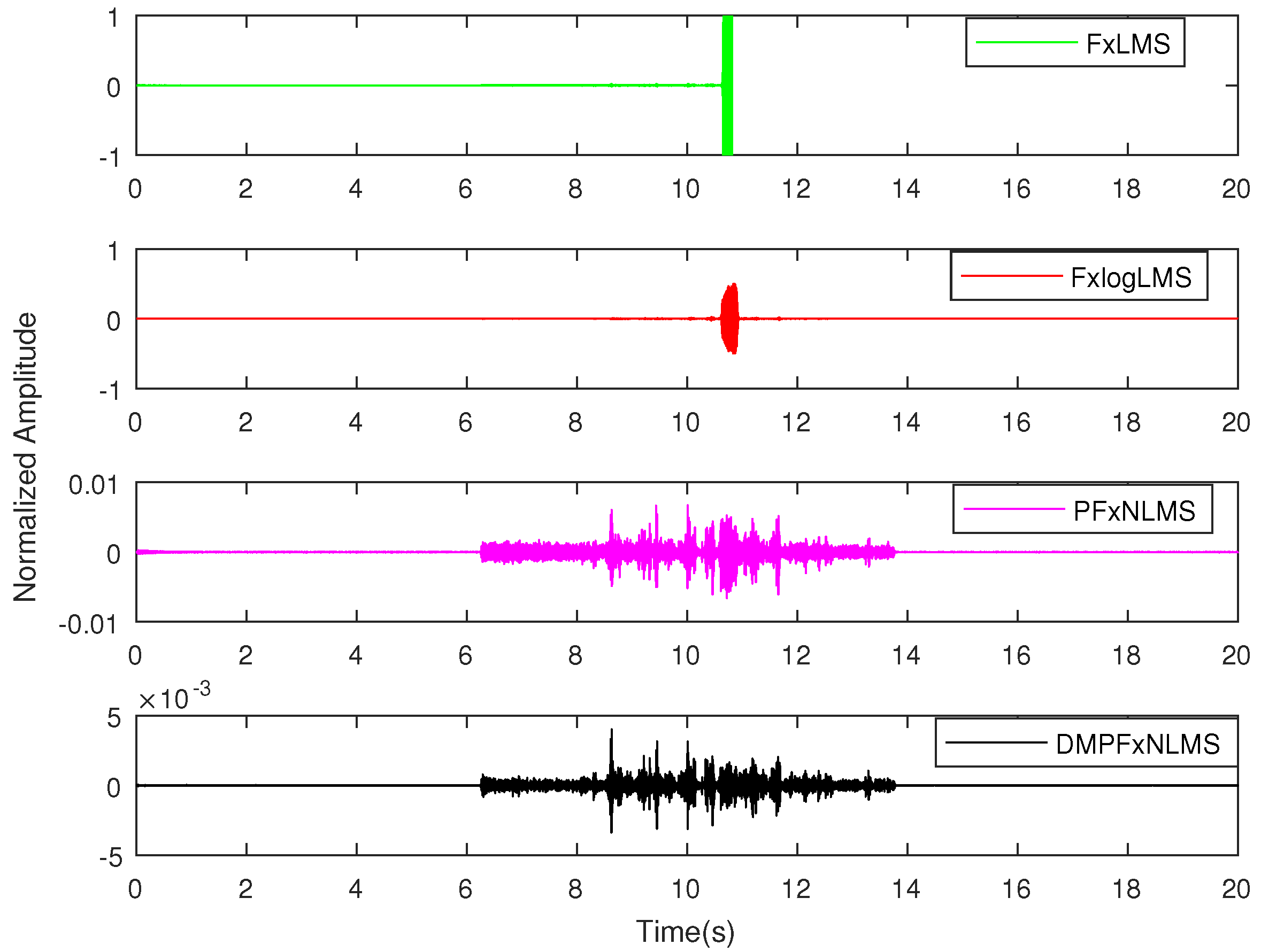
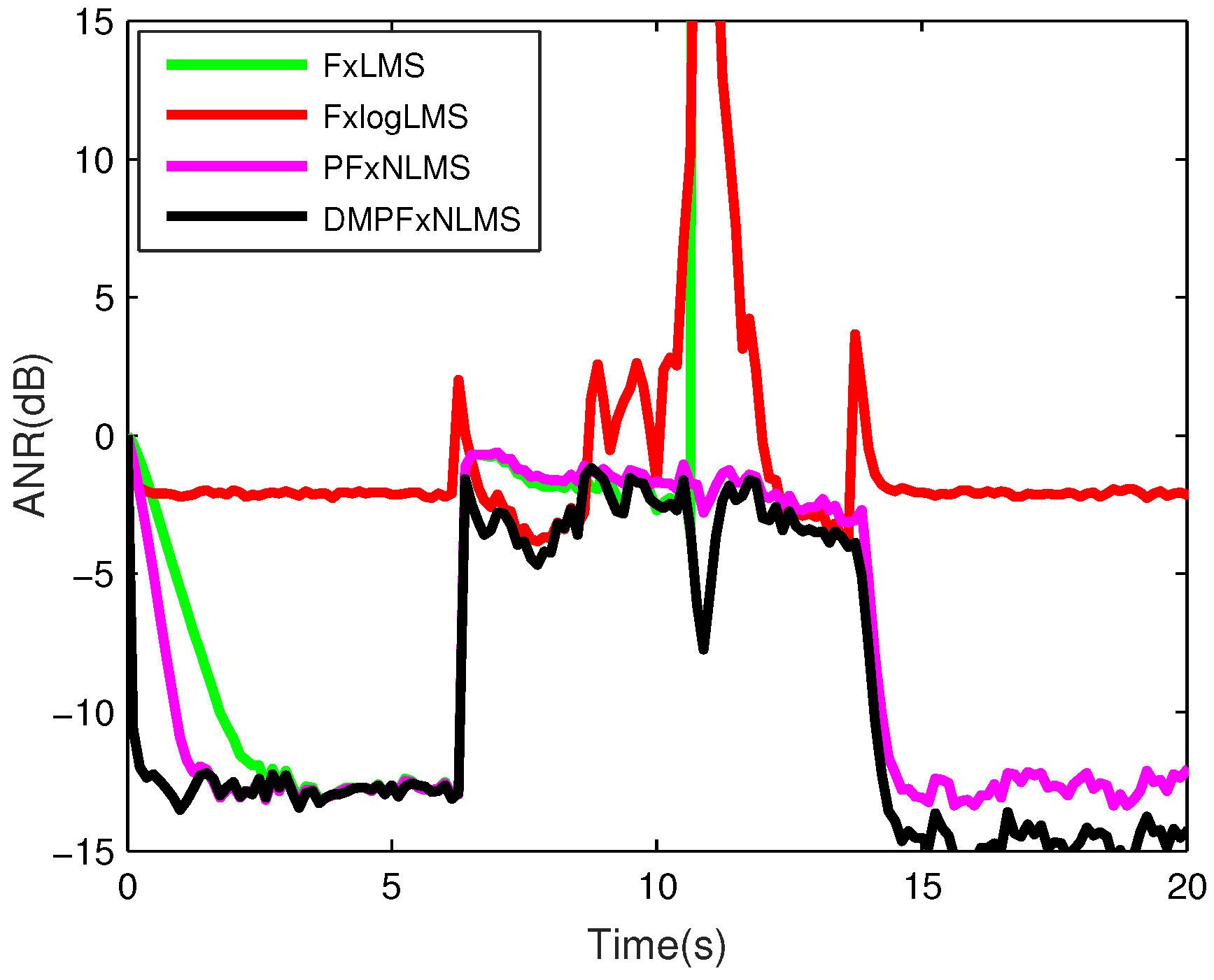
The error learning curves are shown in Figure 11. The FxLMS nearly diverged at 11 s, thus it was stopped manually after that time. It shows that DMPFxNLMS had better attenuation performance than FxlogLMS and PFxNLMS. To show clearly, the ANR performance was considered to give further results in Figure 12.

In Figure 12, the attenuation of FxLMS was inferior to that of other methods applied in this experiment when impulsive interference occurred, it diverged at about 11 s, which also confirmed the conclusion in [8,9,10,11,12,13,14,15] theoretical analysis that the FxLMS cannot cancel impulsive noise. Although the FxlogLMS could maintain the steady state after the impulsive interference, the average attenuation of it was inferior to that of PFxNLMS(Opt) and DMPFxNLMS. Comparing to PFxNLMS(Opt), DMPFxNLMS had a better initial convergence rate. Between 6 s and 15 s, it performed more stably in this experiment. When the impulsive interference disappeared, it had better average attenuation than the PFxNLMS. These proved that the proposed DMPFxNLMS had better performance in the Gaussian noise environment with accidental impulsive interferences.

5. Conclusions

In this paper, a novel adaptive state detector-based post-filtering active control (DMPFxNLMS) algorithm is proposed to achieve ANC in both non-impulsive and impulsive noise environment. An adaptive Gaussian core is introduced that allows the convergence rate of the weight vector to be raised and lowered more quickly than conventional methods when the value of the feedback signal $e\left(n\right)$ increases and decreases in fast tracking mode. A novel state detector is also developed to keep robust for the adaptive filter when the divergence of $e\left(n\right)$ is barely acceptable, and its feasibility is proved by theoretical analysis. Simulations and experimental results show that the proposed DMPFxNLMS algorithm can provide faster tracking than the PFxNLMS algorithm using optimal parameter in non-impulsive interference environment and have better robust performance than FxRMC and FxlogMLS algorithms. Moreover, the DMPFxNLMS algorithm also has less computational load than FxRMC algorithm. Therefore, the proposed DMPFxNLMS algorithm is able to provide better ANC performance in Gaussian environment with impulsive interference.

References

- Kuo, S.M.; Morgan, D.R. Active Noise Control Systems: Algorithms and DSP Implementations; Wiley: New York, NY, USA, 1996. [Google Scholar]
- Zimmermann, M.; Dostert, K. Analysis and modelling of impulsive noise in broad-band powerline communications. IEEE Trans. Electromagn. Compat. 2002, 44, 249–258. [Google Scholar] [CrossRef]
- Lui, L.; Gujjula, S.; Thanigai, P.; Kuo, S.M. Still in Womb: Intrauterine acoustic embedded active noise control for infant incubators. Adv. Acoust. Vib. 2008, 10. [Google Scholar] [CrossRef]
- Georgiou, P.G.; Tsakalides, P.; Kyriakakis, C. Alpha-stable modeling of noise and robust time-delay estimation in the presence of impulsive noise. IEEE Trans. Multimed. 1999, 10, 291–301. [Google Scholar] [CrossRef]
- Leahy, R.; Zhou, Z.; Hsu, Y.C. Adaptive filtering of stable processes for active attenuation of impulsive noise. In Proceedings of the 1995 International Conference on Acoustics, Speech, and Signal Processing, Detroit, MI, USA, 9–12 May 1995; pp. 2983–2986. [Google Scholar]
- Sun, X.; Kuo, S.M.; Meng, G.A. Adaptive algorithm for active control of impulsive noise. J. Sound Vib. 2006, 291, 516–522. [Google Scholar] [CrossRef]
- Akhtar, M.T.; Mitsuhashi, W. Improving performance of FxLMS algorithm for active noise control of impulsive noise. J. Sound Vib. 2009, 327, 647–656. [Google Scholar] [CrossRef]
- Wu, L.F.; He, H.S.; Qiu, X. An active impulsive noise control algorithm with logarithmic transformation. IEEE Trans. Audio Speech Lang. 2011, 19, 1041–1044. [Google Scholar] [CrossRef]
- Li, P.; Yu, X. Active noise cancellation algorithms for impulsive noise. Mech. Syst. Signal Proc. 2013, 36, 630–635. [Google Scholar] [CrossRef] [PubMed]
- Tan, L.; Jiang, J. Active control of impulsive noise using a nonlinear companding function. Mech. Syst. Signal Proc. 2015, 58, 29–40. [Google Scholar] [CrossRef]
- Al-Sayed, S.; Zoubir, A.M.; Sayed, A.H. Robust adaptation in impulsive noise. IEEE Trans. Signal Process. 2016, 65, 2851–2865. [Google Scholar] [CrossRef]
- Akhtar, M.T.; Mitsuhashi, W. Improving robustness of filtered-x least mean p-power algorithm for active attenuation of standard symmetric-α-stable impulsive noise. Appl. Acoust. 2011, 72, 688–694. [Google Scholar] [CrossRef]
- Wu, L.F.; Qiu, X. Active impulsive noise control algorithm with post adaptive filter coefficient filtering. IET Signal Process. 2013, 7, 515–521. [Google Scholar] [CrossRef]
- Bergamasco, M.; Della Rossa, F.; Piroddi, L. Active noise control with on-line estimation of non-Gaussian noise characteristics. J. Sound Vib. 2012, 331, 27–40. [Google Scholar] [CrossRef]
- Lu, L.; Zhao, H. Active noise control using maximum correntropy with adaptive kernel size. Mech. Syst. Signal Proc. 2017, 87, 180–191. [Google Scholar] [CrossRef]
- Mahmood, A.; Chitre, M. Optimal and Near-Optimal Detection in Bursty Impulsive Noise. IEEE J. Ocean. Eng. 2017, 42, 639–653. [Google Scholar] [CrossRef]
- Otsu, N. A threshold selection method from gray-level histograms. IEEE Syst. Man Cyben. B 1979, 9, 62–66. [Google Scholar] [CrossRef]
- Nikias, C.L.; Shao, M. Signal Processing with Alpha-Stable Distributions and Applications; Wiley-Interscience: New York, NY, USA, 1995. [Google Scholar]
- Liu, W.; Pokharel, P.P.; Principe, J.C. Correntropy: Properties and applications in non-gaussian signal processing. IEEE Trans. Signal Process. 2007, 55, 5286–5298. [Google Scholar] [CrossRef]
- Zhou, Y.; Yin, Y.; Zhang, Q. An optimal repetitive control algorithm for periodic impulsive noise attenuation in a non-minimum phase ANC system. Appl. Acoust. 2013, 74, 1175–1181. [Google Scholar] [CrossRef]
- Sun, G.; Li, M.; Lim, T.C. A family of threshold based robust adaptive algorithms for active impulsive noise control. Appl. Acoust. 2015, 97, 30–36. [Google Scholar] [CrossRef]
- Mirza, A.; Zeb, A.; Sheikh, S.A. Robust adaptive algorithm for active control of impulsive noise. EURASIP J. Adv. Signal Process. 2016, 44. [Google Scholar] [CrossRef]
- Kurian, N.C.; Patel, K.; George, N.V. Robust active noise control: An information theoretic learning approach. Appl. Acoust. 2017, 117, 180–184. [Google Scholar] [CrossRef]
- Luo, L.; Sun, J. A novel bilinear functional link neural network filter for nonlinear active noise control. Appl. Soft. Comput. 2018, 68, 636–650. [Google Scholar] [CrossRef]
- He, J.; Lam, B.; Shi, D.; Gan, W.S. Exploiting the Underdetermined System in Multichannel Active Noise Control for Open Windows. Appl. Sci. 2019, 9, 390. [Google Scholar] [CrossRef]
Figure 1.
Block diagram of the feed-forward ANC systems in a duct.
Figure 2.
Block diagram of the proposed DMPFxNLMS algorithm.
Figure 3.
Frequency responses of the primary path and secondary path for a real duct ANC system.
Figure 4.
Selection of optimal for PFxNLMS. (a) Reference signal in time domain; (b) ANR performance.
Figure 5.
Performance comparison when impulsive interference (a) ANR curves; (b) changing process of .
Figure 6.
Figure 7.
ANR performance (a) interference amplifying 15 dB; (b) interference amplifying 5 dB.
Figure 8.
Robustness analysis (a) ANR curves; (b) changing process of ; (c) Euclidean norm of weight vector .
Figure 9.
Diagram of the real-time experiment.
Figure 10.
Reference signal of real-time experiment (a) time domain; (b) frequency domain.
Figure 11.
Performance comparison of noise in error learning curves.
Figure 12.
ANR performance comparison of the real-time experiment.