Structural Methodologies for Distributed Fault Detection and Isolation


1
Industrial AI Lab, Hitachi America, Ltd., Santa Clara, CA 95054, USA
2
Institute for Software Integrated Systems, Dept. of EECS/ISIS, Vanderbilt University, Nashville, TN 37212, USA
3
Department of Electrical Engineering, Linköping University, 58183 Linköping, Sweden
*
Author to whom correspondence should be addressed.
Appl. Sci. 2019, 9(7), 1286; https://doi.org/10.3390/app9071286
Submission received: 5 January 2019
/
Revised: 26 February 2019
/
Accepted: 13 March 2019
/
Published: 27 March 2019
(This article belongs to the Special Issue Fault Detection and Diagnosis in Mechatronics Systems)
Abstract
:The increasing complexity and size of cyber-physical systems (e.g., aircraft, manufacturing processes, and power generation plants) is making it hard to develop centralized diagnosers that are reliable and efficient. In addition, advances in networking technology, along with the availability of inexpensive sensors and processors, are causing a shift in focus from centralized to more distributed diagnosers. This paper develops two structural approaches for distributed fault detection and isolation. The first method uses redundant equation sets for residual generation, referred to as minimal structurally-over-determined sets, and the second is based on the original model equations. We compare the diagnosis performance of the two algorithms and clarify the pros and cons of each method. A case study is used to demonstrate the two methods, and the results are discussed together with directions for future work.
1. Introduction
As the complexity of industrial systems grows, system monitoring and fault diagnosis systems are becoming essential to assure system reliability and functional safety; see for example [1,2] and the references therein. Safety-critical systems must detect and isolate faults quickly and reliably to enable effective safety maneuvers and fault-tolerant control so as not to endanger operations and human lives [3].
Traditional approaches have focused on designing centralized diagnosers for complex systems, e.g., the Aircraft Diagnostic and Maintenance Systems (ADMS) used on modern aircraft systems [4,5]. However, since many industrial applications involve large dynamic systems with many subsystems, distributed approaches to fault detection and isolation are becoming necessary for a number of reasons [6]. Centralized diagnosers are less reliable because they create a single point of failure, and designing centralized diagnosers for large, complex systems may become computationally intractable. Transferring sensor data from the distributed subsystems to a central fault diagnosis unit can become error prone, for example because of packet losses and networking delays, which can then affect the accuracy and timeliness of diagnosis decisions [7]. Furthermore, from a practical point of view, different subsystems are designed by different manufacturers, who may not be willing to pass along all of their knowledge of the subsystems to the system integrator to protect their intellectual property. This makes it difficult for the system integrator to design centralized diagnosers since they to do not have access to subsystem models.
A number of approaches have been developed for distributed fault detection and isolation in discrete event systems. In the simplest case, a group of distributed fault detection and isolation approaches considers each subsystem as a node that reports its state as “OK” or “faulty” without providing any details of the nature of the fault and how it was inferred. This approach is prevalent for wireless sensor networks [8] and computer network [9] diagnosis. For most systems that exhibit hybrid and continuous behaviors, distributed fault detection and isolation is more complicated. In these systems, a subsystem has several components, and a fault could occur in a sensor, actuator, or other components in the subsystem. Therefore, it is not enough to simply declare a subsystem as “OK” or “faulty,” since the isolation of component faults requires deeper reasoning processes. Shames et al. [10] used a bank of unknown input observers for distributed Fault Detection and Isolation (FDI) in time-invariant linear systems. A three-layer distributed diagnosis architecture design was proposed by [11]. Chanthery et al. [12] proposed a distributed residual generation and computation approach for distributed diagnosis.
To achieve accurate fault detection and isolation of a known set of potential faults in a distributed framework, subsystems may have to share data so that the necessary residuals may be derived for fault isolation. Roychoudhury et al. [13] developed an algorithm that searches for the minimal number of additional external measurements to add to each local diagnoser in order to make all faults detectable and isolable in that subsystem. Daigle et al. [14] used a similar approach for distributed fault detection and isolation in mobile robots. Bregon et al. [15] used breadth-first search to find the minimum number of measurements to add to each subsystem to make all the faults detectable and isolable by using information from all local diagnosers. The algorithm guarantees minimum communication among subsystems; however, it is exponential in the number of system measurements. To address this problem, we have proposed a greedy search algorithm that is computationally efficient, but suboptimal. Ferrari et al. [7,16] proposed a similar robust distributed fault detection and identification approach, but they did not address the problem of determining the minimum number of required shared variables between the subsystems.
In this paper, we propose two general approaches for designing a set of distributed diagnosers that together have the same diagnosability performance as centralized approaches: (1) a Minimal Structurally-Over-determined (MSO)-based approach and (2) an equation-based approach. Some of our previous work [17,18] presented an initial approach and results for our distributed diagnosis approach. In this paper, we present the problem formulations, the proposed algorithms, and the accompanying proofs for the hypotheses on which these algorithms are based in more detail. We compare the computational complexities and the application of these algorithms to a testbed: the spacecraft electrical power distribution system [19]. The advantages and disadvantages of each algorithm are discussed to help the health monitoring engineers select the proper approach for a given application.
The first approach uses Minimal Structurally-Over-determined (MSO) set selection [20] and provides globally correct diagnosis results while minimizing the number of measurements shared between different subsystems. Each MSO set used for residual generation represents an analytical redundancy relation in the system [20,21]; however, the total number of MSO sets is exponential in terms of the system measurements. To avoid the computational complexity of dealing with a large number of MSO sets, we propose a second algorithm for designing distributed diagnosers that is based on system equations. This solution is computationally efficient, and its solution matches the diagnosability capabilities of a centralized diagnoser. Moreover, the equation-based method does not require access to the global model for diagnoser design, which makes it applicable to large, complex systems, where global system models are likely to be unavailable or unknown.
The rest of this paper is organized as follows. Section 2 presents basic definitions and the running example we use in the paper. Section 3 presents the MSO-based distributed diagnosis approach, and Section 4 presents the equation-based approach. Section 5 discusses the case study, and Section 6 presents the advantages and disadvantages of each approach along with directions for future work.
2. Basic Definitions and Running Example
This section introduces the basic concepts associated with the distributed diagnosis of dynamic systems.
Definition 1 (System model).
A system model S is a four-tuple: (V, M, E, F), where V is the set of variables, M is the set of measurements, E is the set of equations, and F is the set of system faults.
It is assumed that the sets of V and E are sufficient to define the behavior of the system. The system S is partitioned into n subsystems, , where each subsystem model is defined as:
Definition 2 (Subsystem model).
A subsystem model () associated with a system model, S, is also a four-tuple: (, , , ), where , , , and . Furthermore, .
We note that a variable can be shared between two or more subsystems describing the connection between the different subsystems.
Example 1.
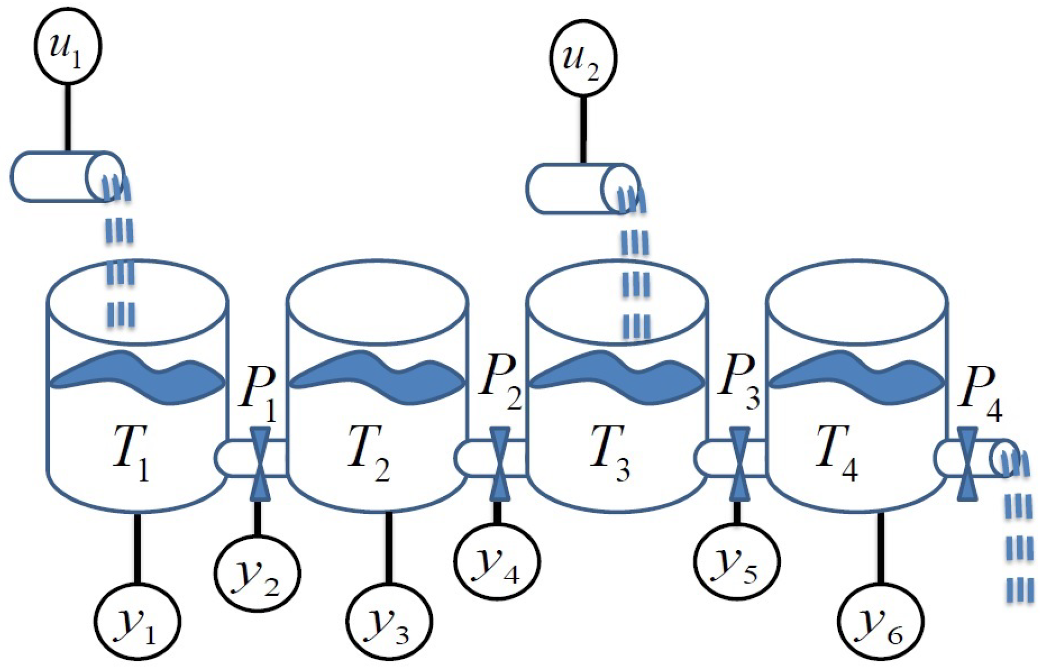
A four-tank system is used as a running example in the paper; see Figure 1. The system is assumed to be divided into four non-overlapping subsystems, where each subsystem is constituted of one tank and the outlet pipe to its right. Two of the subsystems, 1 and 3, also have external inflows into their tanks. Associated with each subsystem is a set of measurements, , that are shown as encircled variables in the figure.
The first subsystem, , in the running example is described by the following set of equations:
defines the set of equations; defines the set of subsystem unknown variables; defines the set of subsystem known variables (measurements); and defines the set of faults associated with this subsystem model. It is assumed that the system parameters (, and of the first subsystem) are known. This model representation is used to emphasize the model structure, which is useful, for example, when analyzing structural fault detectability and isolability properties [2].
Similarly, the three other subsystem models are defined by the following equations:
In the equations, represents the pressure in tank i, and represents the liquid flow through the connecting pipe associated with the adjoining tanks. represents the inflow into tank i. The capacity of tank i is represented as , and pipe resistance is given by . The fault parameters are modeled by . Fault represents a leak in Tank 1; represents a clog in the connecting pipe to the right of Tank 1; represents a leak in Tank 2; represents a clog in the connecting pipe to the right of Tank 2; represents a clog in the connecting pipe to the right of Tank 3; and represents a leak in Tank 4.
The subsystem equations as described in Example 1 take on a general form; as examples, they may be expressed as state space equations, implicit differential equations, etc. The following definitions describe connections between subsystems.
Definition 3 (First order connected subsystems).
Two subsystems, and , are first order connected if and only if they have at least one shared variable.
Definition 4 ( order connected subsystems).
Two subsystems, and , are order connected if there exists a subsystem model that is order connected to and is first-order connected to , or is order connected to and is first-order connected to .
Example 2.
In the four-tank example, subsystems and are first order connected, and their shared variables are . Similarly, and are second order connected because both of them are first order connected to .
In this paper, MSO sets are used as the primary approach for FDI and defined as follows [20]:
Definition 5.
(Structural over-determined set) Consider a set of equations and its associated variables, measurements, and faults: . This set of equations is structurally over-determined (SO) if the cardinality of the set is greater than the cardinality of set , i.e., .
Definition 6.
(Minimal Structurally-Over-determined (MSO) set) A set of over-determined equations is minimal structurally-over-determined if it has no subset of structurally-over-determined equations.
The MSO sets are minimal sets of equations that can be used to generate residuals, for example by using the Fault diagnosis toolbox developed by Frisk and Krysander [22]. MSO sets represent redundant equation sets that capture the redundancies in the system: . For example, , where , , , and represent an MSO set in subsystem (1) of our running example. For brevity and simplification, we simply say a specific equation, variable, measurement, or fault is a member of an MSO in the rest of the paper, e.g., . Each MSO set represents a part of the system model that can be used to design a residual that is only sensitive to certain faults. A set of MSO sets can be used to generate residuals that together can isolate a set of faults.
To discuss the fault detectability and isolability properties of the global system and its subsystems, we define global and local fault detectability and isolability as follows.
Definition 7.
(Globally-detectable fault) A fault f∈F is globally detectable in system S if there is a minimal structurally over-determined set in the system, such that f∈.
Definition 8.
(Locally-detectable fault) A fault f∈ is locally detectable in subsystem if there is a minimal structurally over-determined set in the subsystem such that f∈
Example 3.
Fault in (1) is locally detectable because . However, is not locally detectable because there is no MSO set in this subsystem that includes . To detect locally, the diagnosis subsystem requires additional measurements.
Definition 9.
(Globally-isolable fault) A fault ∈F is globally isolable from fault ∈F if there exists a minimal structurally-over-determined set in the system S, such that ∈ and ∉.
Definition 10.
(Locally-isolable fault) A fault ∈ is locally isolable from fault ∈F if there exists a minimal structurally-over-determined set in subsystem , such that ∈ and ∉.
Note that if a fault is locally detectable in a subsystem , it is globally detectable as well, and if a fault is locally isolable from a fault , it is globally isolable from , as well.
3. MSO-Based Distributed Fault Detection and Isolation
3.1. Problem Formulation
The objective in this work is to design a set of distributed diagnosers that together have the same diagnosability as a centralized diagnoser. This means that a distributed approach should detect any fault that is globally detectable and isolate any pair of faults that are globally isolable. In the ideal case, there are enough MSO sets in each subsystem to detect and isolate all of its faults, . In that case, no exchange of information is necessary between the different diagnosers. If the independence among diagnosers does not hold, the different subsystems need to share some sensor data with each other to be able to detect and isolate the faults.
To address this problem in an efficient way, an integrated approach is derived to select a set of MSO sets for each subsystem that guarantee full diagnosability and minimum exchange of measurements among subsystems. The general idea is to augment each subsystem with additional measurements that are typically acquired from the (nearest) neighbors of the subsystem, such that all of the faults associated with the extended subsystem model are detectable and isolable. In the worst case, all of the measurements from another subsystem may have to be included to make the current subsystem diagnosable. When such a situation occurs, we say the two subsystems are merged and represented by a common diagnoser; therefore, the total number of independent distributed diagnosers may be less than k.
Let denote the set of candidate MSO sets for the system S. For each subsystem , the objective is to develop an algorithm to select a subset of s that guarantees maximal structural detectability and isolability for faults associated with the subsystem, while using a minimum number of measurements from the other subsystems in the system to assure the equivalence of local and global diagnosability, i.e.,
where represents the set of measurement we need to communicate to the subsystem and represents the set of measurement subsystem that will be used to diagnose all faults associated with it. M represents the set of all measurements in the system. For a given set of measurements, X, represents the set of detectable faults, and represents the set of isolable faults in and .
3.2. MSO Set Selection for Distributed Fault Detection
For the situation in which the global model is known, in Equation (3) is the set of all system measurements. Let us assume we can generate r MSO sets given M: .
Our goal is to design an algorithm that selects in a way that requires a minimum number of additional measurements , i.e., measurements from the system not belonging to subsystem , to make all its faults globally detectable and isolable, if possible. Note that this is equivalent to the set-covering problem, which is NP-complete. In the past, heuristic search methods have been adopted for solving this problem, for example a Temporal Causal Graph (TCG) approach was used in [13]. In this paper, the problem is formulated as a Binary Integer Linear Programming (BILP) problem [23]:
where vector c represents the cost weights, matrix A and vector b define linear constraints, x represents the variables, represents the binary variables, and represents a scalar binary variable [24].
There are several tools available for solving this problem, e.g., branch and bound algorithms [25] and branch and cut algorithms [26] (see, for example, http://www.mathworks.com/help/optim/ug/mixed-integer-linear-programming-algorithms.html in the MATLAB™ linear integer programming toolbox).
To formulate the problem (3) as a BILP problem, a binary variable : is defined for measurement in the system as follows:
where is the answer to Problem (3). An additional binary : , is used for MSO set in the system as follows.
Minimizing the number of measurements used from the other subsystems, this is formulated in the following cost function c as:
where l is the number of system measurements and r is the number of MSO sets in the system. To determine the set of measurements and selected MSO sets in each distributed diagnoser, a BILP algorithm with binary variables should be solved for the subsystem.
Consider subsystem with local faults and the set of system faults, F. Each local fault has to be locally detectable. Given Definition 8, local detectability of all the faults is achieved using the following constraints in the optimization problem (4).
By considering for , where g is the number of faults in , the solution will contain at least one MSO set to detect each fault.
The following constraint is added:
is used to isolate from another fault . Setting for , where h is the number of faults in the system, , will make sure that there is at least one MSO set to isolate each of the subsystem faults from the other faults in the system.
Using an MSO set is equivalent to using the measurements that are included in the MSO set. For example, using from the water tank example in a subsystem diagnoser requires three measurements transmitted to that subsystem. Therefore, a set of constraints is included that capture the relationship between the measurements and MSO sets in the distributed diagnosis system.
Equation (10) represents this set of constraints in the A matrix.
where is the cardinality number of the set of measurements in and is the number of measurements in the system. Furthermore, for , where r is the number of MSO sets in the system.
Example 4.
The water tank system has 165 MSO sets. The entire system includes eight measurements, where subsystem includes three measurements. has two faults of interest, and the goal is to be able to isolate them from the other six faults in the complete system. For the optimization problem (4) for , matrix , i.e., two local detectability constraints, 10 local isolability constraints, and 165 constraints to capture the relationship between the MSO sets and the measurements and 173 columns corresponding to the eight measurements and 165 MSO sets.
Table 1 shows the set of measurements to add for each of the subsystem diagnosers to achieve maximum possible detectability and isolability. To find the optimum measurements, the optimization problem (4) has been solved for each subsystem.
Subsystem initially has three measurements . To achieve global diagnosability for its faults, must be shared with its diagnoser from subsystem . Subsystem is the only subsystem that shares a variable with a second order connected subsystem. All the other subsystems only need to communicate with their first order connected subsystems.
In general, the worst case scenario for a system with connected subsystems will typically require a large number of measurements from other subsystems to be communicated to each subsystem diagnoser. In those situations, distributed subsystem diagnosers help overcome the single point of failure problem, but each subsystem diagnoser may require a large number of measurements to be communicated to it from all of the other subsystems.
Even though there are efficient algorithms to solve BILP problems, this approach will not scale up for larger systems, since the search space is exponential in the number of MSO sets , even if the subsystem diagnoser design is performed off-line. In addition to the computational complexity, the availability of global models for large, complex systems is unlikely because of the issues discussed in Section 1. To overcome this problem, a heuristic search strategy is proposed based on an incremental search algorithm that works with the original system equations instead of MSO sets.
4. Equation-Based Distributed Fault Detection and Isolation
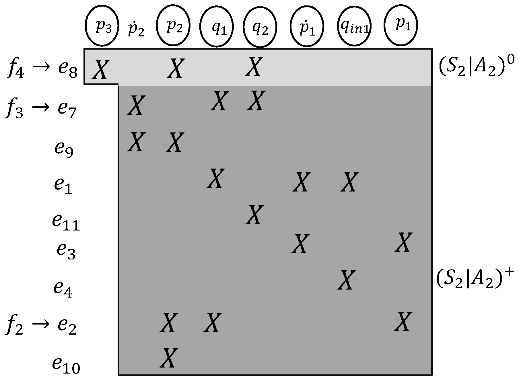
To avoid the computational complexity of the MSO-based algorithm, in the previous section, a distributed diagnosis method that works directly with the system of equations is proposed. To recap from earlier work [27], a structural model representation is used. A structural model describes which variables are included in which model equations. A useful tool is the Dulmage–Mendelsohn (DM) decomposition that decomposes a system model into three parts: (1) under-determined, (2) exactly determined, and (3) over-determined. The over-determined part introduces redundancy in the system description and forms the basis for fault detection and isolation [2]. Figure 2 shows the DM decomposition of subsystem in the running example.
The figure represents the set of equations in the just determined part, , the set of equations in the over-determined part, , and the set of unknown variables in each equation.
The shared variables are shown as encircled variables in the figure. Without loss of generality, it is assumed that every fault parameter is included in exactly one equation, i.e., each fault f appears in one equation . This is not a restricting assumption because if a fault is included in more than one equation, we can replace the fault signal by a new variable and add a new equation where the new variable is equal to the fault. Similar to the definitions of detectability and isolability for a structural model in, e.g., [20], local detectability and isolability can be defined as:
Definition 11.
(Locally detectable) A fault f∈ is locally detectable in subsystem if ∈, where is the over-determined part of subsystem .
Definition 12.
(Locally isolable) A fault ∈ is locally isolable from fault ∈F if ∈, where is the over-determined part of subsystem without equation .
Note that these definitions are equivalent to Definitions 8 and 10 since an MSO set is an over-determined equation set.
Consider Definition 11 and Figure 2. Fault is locally detectable because ∈, but is not locally detectable since . To expand the over-determined part and make detectable, the diagnosis subsystem needs to include at least one additional equation. The extension to the original subsystem is defined as:
Definition 13.
(Augmented subsystem) Given subsystem and a set of equations, , the augmented subsystem model is (, , , ), where is the union of and the unknown variables that appear in , is the union of and the known variables that appear in , is the union of and , and is the union of and the possible faults associated with .
Example 5.
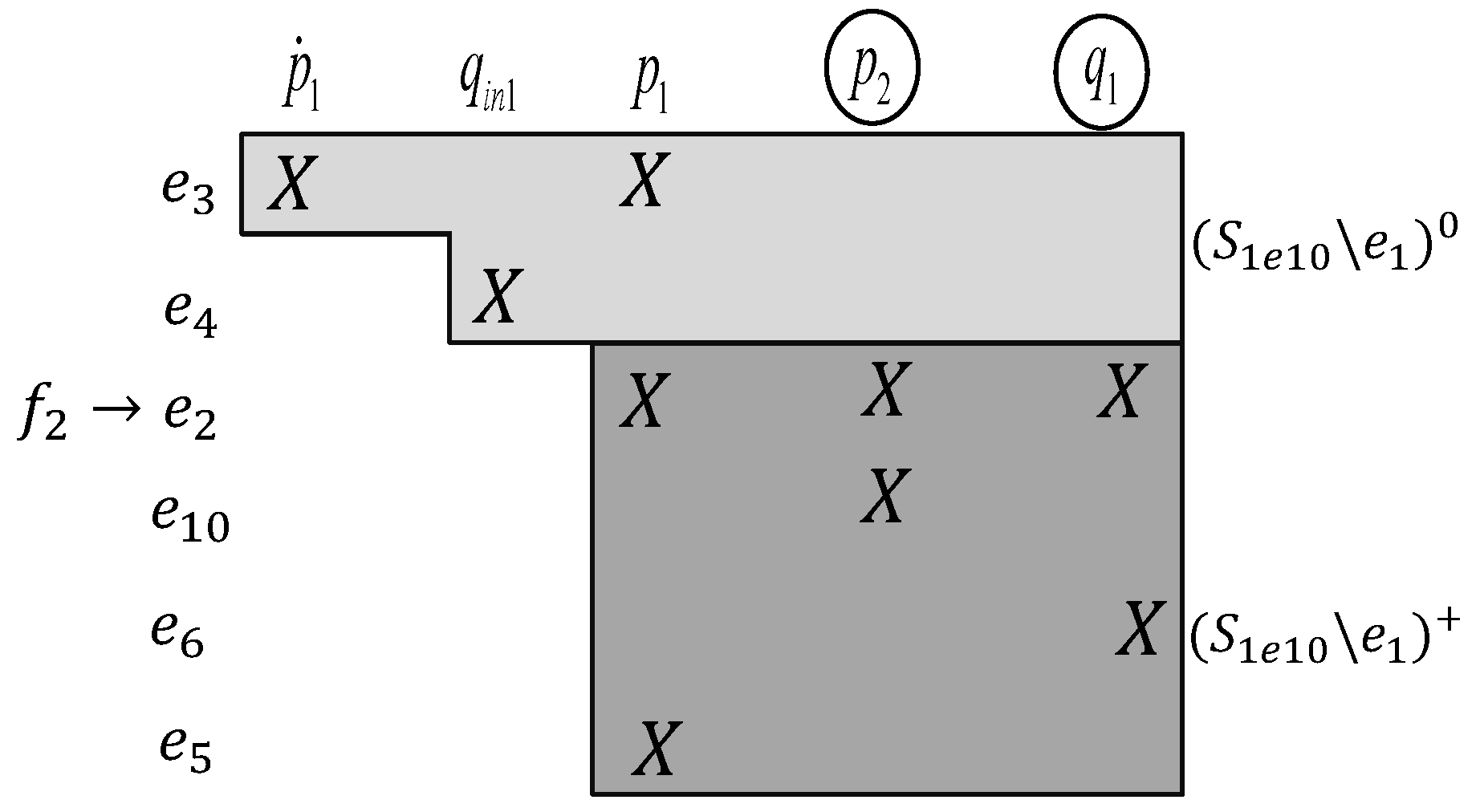
Consider the running example. = (, , , ), where , , , and . Note that did not add any new unknown variables or faults to the subsystem model. Figure 3 represents the DM decomposition of the augmented subsystem, . This figure shows that ∈, and therefore, is locally detectable for the augmented subsystem .
Figure 4 shows DM decomposition of the . Equation is in the over-determined part of the augmented subsystem model; therefore, is locally isolable from in the augmented subsystem.
4.1. Problem Formulation
An equation-based solution approach is formulated for designing a distributed diagnoser. For the given set of subsystems , when there are faults that are not locally detectable or isolable in one or more subsystems, it is necessary to consider the following cases:
- is not locally detectable.
- and are not locally isolable from each other.
- is not locally isolable from and .
The last case represents a scenario where a subsystem fault is not locally isolable from a fault outside of the subsystem. This scenario can happen because a fault occurrence can have consequences beyond the original subsystem. Designing distributed diagnosers that account for these three scenarios is the focus in this section. After addressing each of these situations, we derive an integrated approach to distributed FDI and derive algorithms that apply to complex, dynamic systems made up of a number of subsystems.
For each subsystem, it might be necessary to augment the subsystem model with additional equations that are typically acquired from the neighbors of the subsystem, such that all of the faults associated with the augmented model are locally detectable and isolable. A set of equations is minimal if there is no subset of equations that provides the same detectability and isolability. More formally, the problem of designing a diagnoser for a particular subsystem can be described as follows.
Consider as the set of neighboring subsystems to subsystem . To address the three situations mentioned above, an algorithm is to be developed to find a minimal equation set in that guarantees maximal structural detectability and isolability for subsystems faults , i.e., that solves the optimization problem:
where represents the set of all the equations in , D represents the set of detectable faults in , and I represents the set of isolable faults in from the system faults F.
Example 6.
Consider the first subsystem of the running example , makes and detectable and isolable from all the other faults in the system. Therefore, is a minimal solution to the problem.
In this section, we present a method to make all the faults in a subsystem locally detectable (Situation (1) above). We also discuss the solution to the fault isolability problem (Situation (2) above) and prove that if we address the first situation, the third situation is automatically taken care of.
4.2. Maximum Detectability
Example 7.
Consider subsystem in the four-tank example whose equations are listed in (1). The DM decomposition of this subsystem is shown in Figure 2. is in the just determined part of the subsystem; therefore, the fault is not locally detectable. However, is a shared variable with Subsystem 2. Therefore, an equation from subsystem can be selected, , to make locally detectable in the augmented subsystem, (see Figure 3). Adding measurement equation makes known and, therefore, makes the subsystem over-determined.
Note that a variable that only appears in one subsystem (for example in ) cannot become known by adding equations from other subsystems. Therefore, our ability to increase fault diagnosability is limited to the shared variables in the subsystem. More formally, we can prove the following theorem.
Theorem 1.
Consider local subsystem model = and the set of shared variables in the subsystem. If a fault is not locally detectable in a new subsystem = where all the shared variables are known, f is not globally detectable.
Proof.
If remains in the just determined part or under determined part of the subsystem when all the shared variables have became known, there is no additional equation in the system that can make any of the variables in known. Therefore, the equation cannot be moved to the over-determined part of the structural decomposition. □
Therefore, the maximum detectability that can be achieved in each subsystem cannot be more than the detectability when all the shared variables are known. Using Theorem 1, we develop Algorithm 1 and Algorithm 2 to find an upper bound for the number of detectable faults and isolable fault pairs in each subsystem, respectively. Note that our algorithms do not require any information from the neighboring subsystems.
| Algorithm 1 Detectable faults. |
|
| Algorithm 2 Isolable faults. |
|
Adopting the following strategy, a minimal set of shared variables can be found that guarantees maximum detectability.
- We assume all the shared variables are known. If a fault is not locally detectable when all the shared variables are known, that fault is removed from the list of detectable faults (see Algorithm 1).
- Each shared variable is removed from the list of known variables to the unknown variables one at the time, to evaluate the list of detectable faults. If removing the shared variable from the known variables decreases the number of faults in the list of detectable faults, the shared variable is added back to the list of minimal required shared variables. Otherwise, the shared variable is not needed.
Algorithm 3 presents our method to find a minimal set of required shared variables. The algorithm is initialized with the subsystem model and the set of shared variables (for subsystem , and are unknown shared variables), and this provides a minimal subset of shared variables that makes all the faults detectable in the subsystem. For Subsystem 1, is a possible answer.
| Algorithm 3 Minimal shared variables. |
|
Note that all of the shared unknown variables may not be measured. However, in some cases, it is possible to transfer a set of equations from the neighboring subsystems that can be used with the equations in the subsystem to compute the unknown variables.
4.3. Equation-Based Fault Detection Approach
Given a minimal set of required shared variables, we present our proposed approach to find a minimal set of equations from the neighboring subsystems in order to achieve the maximum possible fault detectability. The procedure is illustrated by solving this problem for subsystem , presented in Equation (2), of the running example, and then generalizing this approach by developing a general algorithm to solve this problem.
Example 8.
The corresponding structural decomposition of is shown in Figure 5.
Subsystem is just determined; therefore, none of the faults are locally detectable. However, and are shared variables with subsystem , and and are shared variables with . Algorithm 3 finds as a minimal set of shared unknown variables, which if transferred from neighboring subsystems, can provide maximum detectability performance.Therefore, to make and locally detectable, the neighboring subsystems are explored to find equations that make the variables and known.
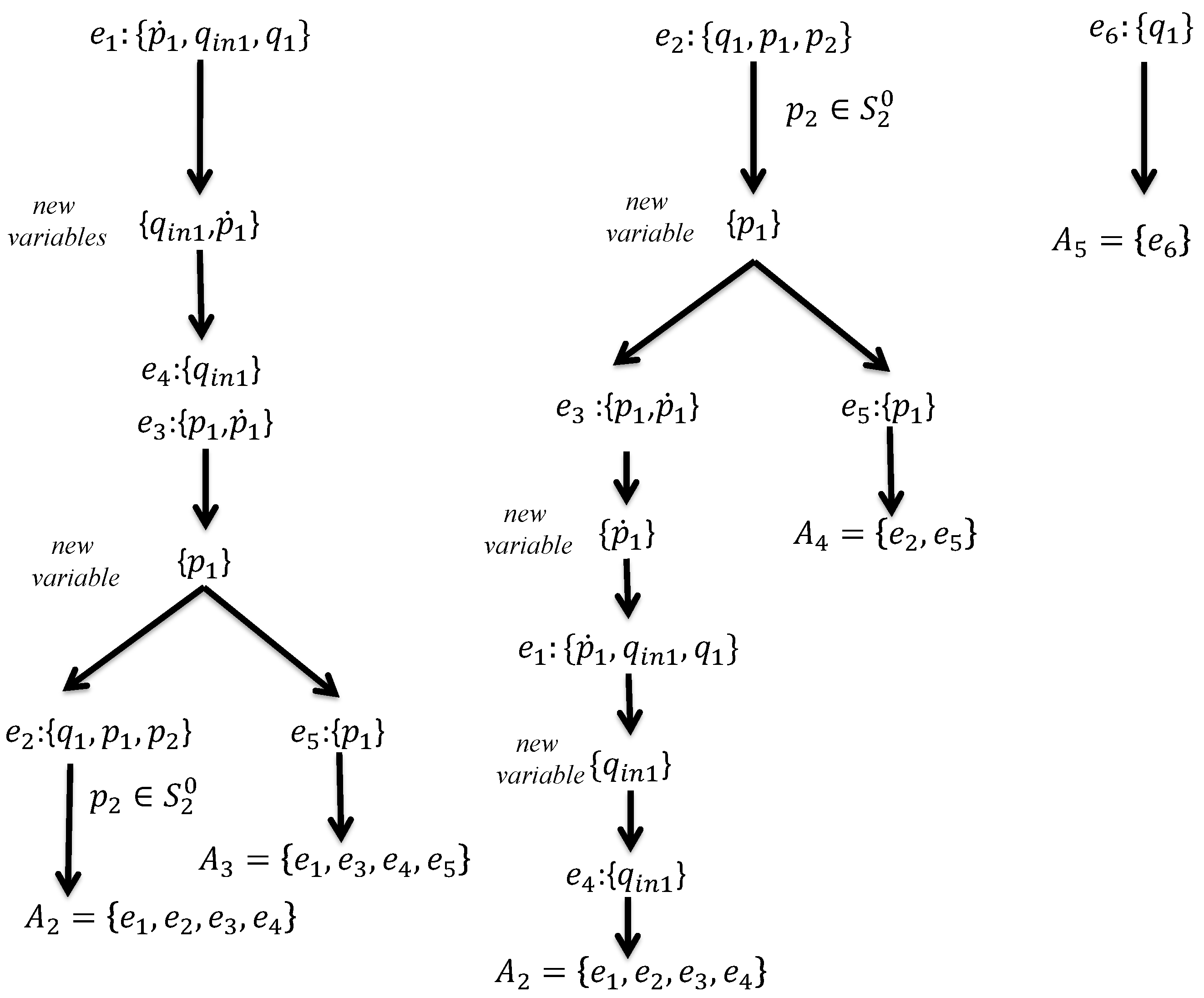
To find a minimal set of just determined equations that includes , we start with all equations in that have . These equations are , , and , as is shown in Figure 6.
Then, for the additional variables in each equation that are not already in , additional equations are included. For equation , two additional equations are needed, one with and the other one with . Finally, another equation is needed where is included. Since , the variable is not considered in this step.
To find the other minimal sets in the example, we keep adding the relative equations to the other sets using the same approach described above. As is shown in Figure 6, by sequentially adding equations to the system, we eventually achieve four sets of minimal constraints: , , , and . Figure 6 represents a matching algorithm. In the previous work in [28], a matching algorithm was introduced for finding a minimal set of equations for detecting each discrete mode change during the hybrid system’s operation. In this paper, a similar approach was applied to find a minimal set of equations from neighboring subsystems for computing each required shared variable as presented as Algorithm 4.
| Algorithm 4 Count matchings. |
|
If we initialize the algorithm with the set of unknown variables (in Figure 6, is the unknown variable), this provides a set of complete matching of variables and equations in the neighboring subsystems that includes the unknown variables.
Example 9.
Figure 7 shows that augmenting with makes detectable. To make locally detectable as well, Algorithm 4 is used to find a minimal set of equations in the neighboring subsystems that includes and augment with those equations.
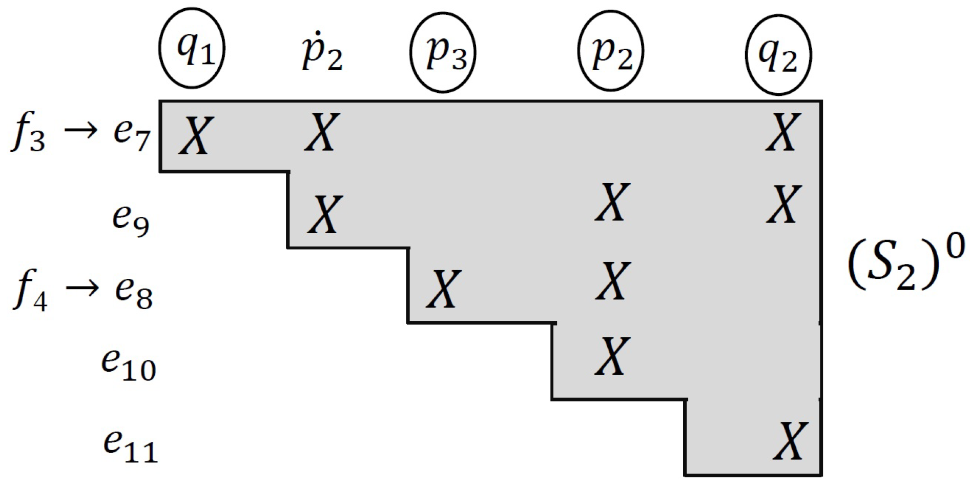
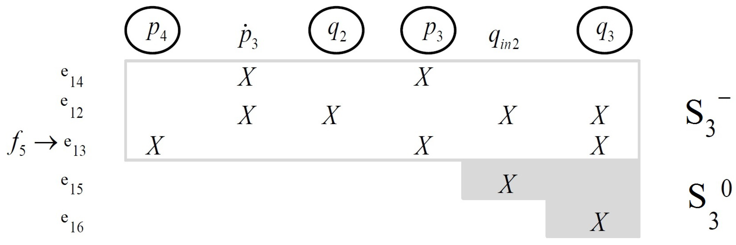
Subsystem is just determined, but a subsystem can have an under-determined part as well. For example, consider subsystem in Equation (2) where the DM decomposition is shown in Figure 8. Fault is in the under-determined part of the structure.
and are in the just determined part of the system, and we can compute them using and , respectively. However, to compute the other four variables in the subsystem, , , , and , we only have three constraints, which makes complete matching between constraints and variables impossible. To make this part of the subsystem just determined, we need to augment a set of equations from the neighboring subsystems.
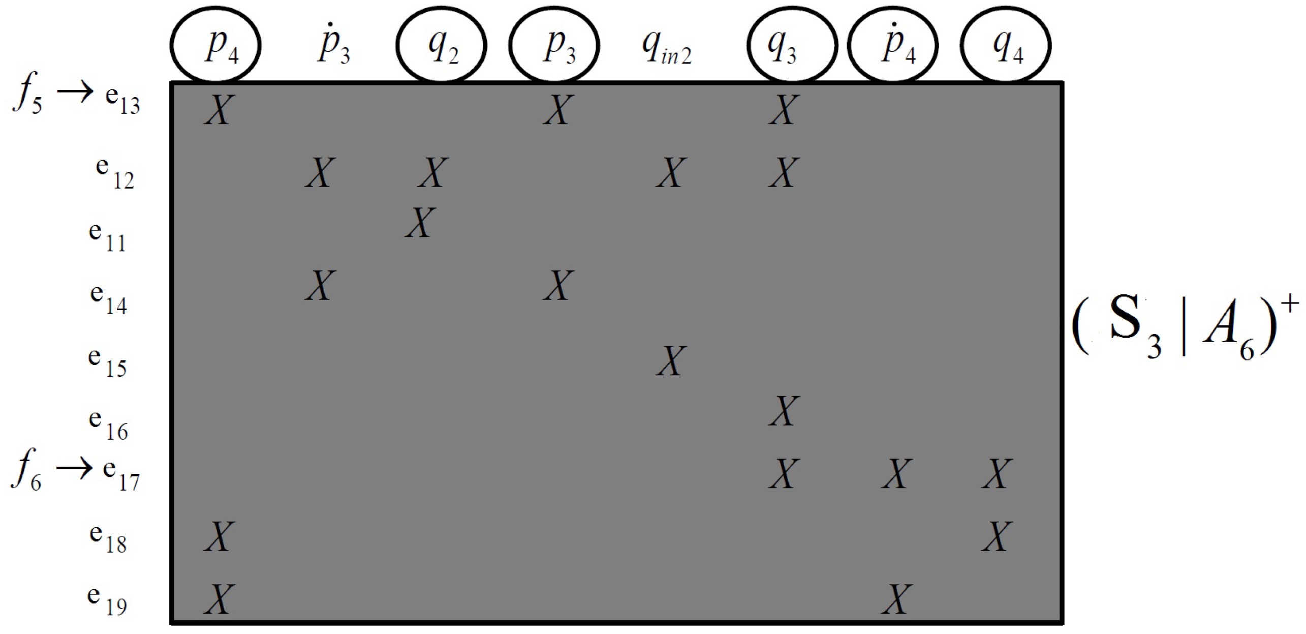
Unlike previous work [18] where an algorithm was developed for subsystems with under-determined parts, Algorithm 3 automatically takes care of this. Using Algorithm 3 gives as a minimal set of required shared variables to make detectable. Having the set of required shared variables, Algorithm 4 gives as a minimal sets of equations from neighboring subsystems can be used to augment to make locally detectable. Figure 9 shows the DM decomposition of .
In some cases, it is possible that an augmented minimal set, , also adds a set of faults to the subsystem model . These faults can be sensor faults or faults in other equations. The following theorem states that these faults are locally detectable in subsystem model .
Theorem 2.
Consider local subsystem model = , and a set of minimal equations that makes set of faults detectable in the augmented subsystem , then the set of faults in the augmented subsystem is locally detectable.
Proof.
The proof of this theorem is straight forward, since the minimal set makes a part of the system that includes the fault over-determined, and the set itself should be in the over-determined part as well. This means the associated faults in the set are detectable. □
For example, is locally detectable in ; see Figure 9. As long as fault detection is considered, the augmented faults do not cause any problem. The fault detection algorithm is summarized in Algorithm 5.
| Algorithm 5 Detectability. |
|
4.4. Equation-Based Fault Isolation Approach
In this subsection, it is assumed that the set of minimal equations to make all the faults locally detectable have been derived as described in the previous subsection. It is clear that the locally-detectable faults in each subsystem are locally isolable from the faults in the other subsystems not included in the augmented subsystem.
Theorem 3.
Consider local subsystem = . If is locally detectable in , then is the locally-isolable form if .
Proof.
Since is detectable, we have , and since , we can say . Therefore, and . □
Considering Theorem 3, it is straight forward to address the isolability problem. For each fault , we remove the associated equation from and all the neighboring subsystems. Then, we use Algorithm 5 to make all the remaining faults in detectable.
Example 10.
In in Figure 9, is isolable from and because they are not in the augmented subsystem and is detectable in this augmented subsystem. To make isolable from , we remove from and . Applying Algorithm 5 to gives as a minimal set that can make detectable.
The augmented subsystem will detect and isolate it from all the other faults in the global system S. Algorithm 6 summarizes the method discussed above.
| Algorithm 6 Diagnosability. |
|
Our proposed approach considers the first order neighboring subsystems of subsystem and augments minimal constraints from them to maximize diagnosability. If the set of first order neighboring subsystems does not have required redundancies to achieve maximum diagnosability, the search process continues to the next higher order of neighboring subsystems, as illustrated in Figure 10. The expansion process will stop when the distributed approach achieves maximum diagnosability, which in the worst case will result in a centralized diagnoser for the whole system. Thus, it is guaranteed that the method will find a distributed set of subsystem diagnosers that achieves the same diagnosability performance as the best centralized diagnoser for the same set of measurements. Algorithm 7 summarizes this approach.
| Algorithm 7 Distributed diagnosis. |
|
The set of equations and measurements that each subsystem in the running example needs from its neighbors to achieve maximum possible detectability and isolability using the equation-based approach are presented in Table 2. Table 2 shows that all the subsystems of the water tank example share measurements with their first order connected subsystems. This is a practical advantage of this algorithm because usually, the subsystems with shared variables are physically closer to each other (corresponding to our definition of nearest neighbors).
Another advantage of this algorithm is that not only do we not need a global model for detecting and isolating the faults, but also, we do not use the global model in the design process of the supervisory system. This makes the approach suitable for large, complex systems, such as aircraft and power plants where the global systems models are likely to be unavailable or are unknown.
4.5. Computational Complexity
The time complexity of Algorithm 5 is mostly governed by Algorithm 4 (Count-Matchings) that has exponential complexity , where is the number of required unknown variables in the subsystem and is the number of equations in the neighboring subsystems. Algorithm 6 calls Algorithm 5 for every fault in the subsystem. Therefore, Algorithm 6 has time complexity for subsystem , where is the number of faults in the subsystem. Note that in the case that no globally-accurate diagnoser can be derived using neighboring subsystems, the solution gradually expands to include all subsystems. Therefore, the time complexity of our proposed method in Algorithm 7 for subsystem i is , where is total number of equations in the system.
In practice, Algorithm 4 finds the answer much faster. For example, consider Figure 6 where Algorithm 4 is searching for a set of equations to solve . As soon as the algorithm reaches an equation that does not have the required unknown variable, the algorithm discards that equation and, therefore, avoids enumerating the rest of the candidate equations in that branch. To achieve even faster solutions, we can sort the equations by the number of their unknown variables before the search. In this way, the algorithm starts with equations with fewer unknown variables and, therefore, has to expand fewer branches on average.
The equation-based solution is exponential in terms of the number of equations in the system. The MSO-based solution is exponential in terms of the number of MSO sets in the system. The total number of MSO sets for fault detection and isolation grows exponentially as the number of measurements increase [29]. Consider Definition 1. The total number of redundancies introduced into the system model is equal to the number of measurements, . Theoretically, each MSO set can include anything from one to measurements. Therefore, the total number of MSO sets, , is proportional to all possible combinations of the measurements:
In general, there are many more MSO sets in a system than equations. For example, the running example in this paper has 20 equations, and the fault diagnosis toolbox generated 165 MSO sets for this system. Therefore, we expect the equation-based approach to solve the problem in a more efficient way, which is demonstrated next.
5. Case Study
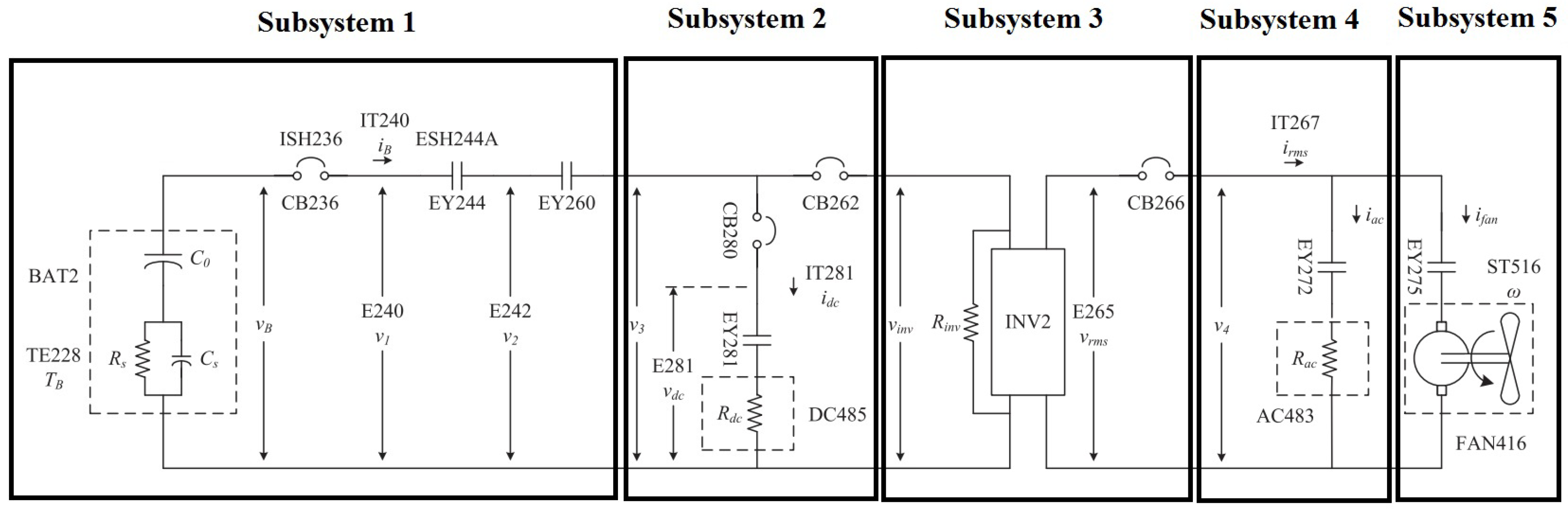
The ADAPT-Lite system is designed to emulate the operation of generic spacecraft electrical power distribution systems [30]. The system has five subsystems: (1) the battery, (2) the Direct Current (DC) electric load, (3) the inverter, (4) the Alternating Current (AC) resistive electric load, and (5) the electric fan as a second inductive load for the AC system (see Figure 11). Seven measurements are made on the system: and represent DC voltage measurements in the system; represents the battery current; represents the inverter AC output voltage; is the inverter AC output current; and is the fan rotational speed. Six faults are considered in the system: and are sensor faults in , and , respectively; represents a fault in the DC load; models inverter faults; represents a fault in the AC load; and is a fan fault. The ADAPT-Lite system has several Circuit Breakers (CB236, CB262, CB266, and CB280), and relays (EY244, EY260, EY281, EY272, and EY275) and, therefore, operates as a hybrid system with multiple modes (configurations).
In previous work [28], we discussed structural diagnosis for hybrid systems. In this paper, we focus on distributed diagnosis. Therefore, we assume all the circuit breakers and relays are on and there is no mode change in the system. The set of equations in each subsystem is derived as follows.
Subsystem 1 (battery): The set of equations:
where is the set of unknown variables in this subsystem, the set of measurements is , represents subsystem faults, and , and are the component parameters in the subsystem. The battery is directly connected to the second subsystem (DC load).
Subsystem 2 (DC load): The DC load is modeled by an electric resistance, . The set of equations for this subsystem is:
where are unknown variables, are measurements, are faults, and is a component parameter in the subsystem. Subsystems 1 and 2 are first order connected, and their shared variables are .
Subsystem 3 (inverter): The inverter converts DC power to AC. When there is no fault in the subsystem and the input voltage, is above 18 V, the output voltage, , stays at 120 V. represents the internal resistance in the inverter, and e is the inverter efficiency coefficient. The set of equation for the subsystem is:
where are unknown variables, is a measurement, is a fault, and are parameters of the subsystem. Subsystems 2 and 3 are first order connected, and their shared variables are . Subsystems 1 and 3 are second order connected because they have no shared variable, and they are both first order connected to the second subsystem.
Subsystem 4 (AC load): Like the DC load, the AC load is modeled as an electric resistance, . The set of equations for this subsystem is:
where are unknown variables, is the measurement, is a fault, and are parameters of the subsystem. Subsystems 3 and 4 are first order connected, and their shared variable is .
Subsystem 5 (electric fan): The fan rotational speed, , is a function of the fan current, . The last subsystem equations are:
where are unknown variables, is a measurement, and is a fault of the subsystem. Fan electrical resistance, , fan inertial, , and fan mechanical resistance, , are the parameters. Subsystems 4 and 5 are first order connected, and is the set of shared variables among these subsystems.
5.1. Distributed Diagnoser Using the MSO-Based Method
For the ADAPT system, there are 258 MSO sets. To find the minimal number of shared measurements, the global MSO set selection algorithm solves an optimization problem for each subsystem. Table 3 shows the set of measurements that needs to be add for each of the subsystem diagnosers to achieve maximum possible detectability and isolability. In the first subsystem, all the faults are locally detectable and isolable, and therefore, this subsystem does not require any additional measurements from the other subsystems. For each of the other subsystems, we have to transfer exactly one measurement to achieve maximum diagnosability.
Table 4 shows the set of MSO sets for each local diagnoser. Note that the global MSO sets’ selection method only minimizes the number of shared variables, but the subsystems may require equations from the other subsystems. For example, the first subsystem in ADAPT does not require any additional measurement to detect and isolate its faults locally; however, as we can see in Table 4, this subsystem requires several equations from the other subsystems to generate residuals.
The total time for finding all MSO sets and solving the optimization problems to find a set of MSO sets for each subsystem with minimum shared variables was 118 s, when the experiment was run on a desktop with an Intel Core i7-4790 3.60-GHz processor.
5.2. Distributed Diagnoser Using the Equation-Based Method
Instead of generating all the MSO sets and selecting a subset of MSO sets for each local diagnoser, Algorithm 7 is used.
The results are shown in Table 5, summarizing the set of equations to augment each subsystem to achieve maximum possible detectability and isolability. In some cases, the first order neighboring subsystems were not enough to detect and isolate all the faults, and the algorithm had to extend to include higher order neighbors. For example, for Subsystem 2, the algorithm cannot find any solution when it considered the first order neighbors (Subsystem 1 and Subsystem 3). Therefore, it extended the search to a second order neighboring subsystem (Subsystem 4).
Table 5 also represents the set of additional measurements that we need to transfer to each ADAPT subsystem. As mentioned earlier, the equation-based algorithm does not guarantee globally-minimum communication. For example, Subsystem 2 required three measurements from other subsystems (see Table 5). However, Table 3 shows that complete diagnosability was achievable by adding only one additional measurement. To detect and isolate faults in each subsystem, the augmented subsystem equations were used to generate MOS sets. Table 6 shows the set of MSO sets for each local diagnoser using the equation-based method. The experiment was run on the same desktop where total execution time was . This demonstrates the computational advantage of this method.
5.3. Designing the Diagnosers
After the augmented subsystem models have been selected, computational tools, for example the fault diagnosis toolbox [22], can be used to generate the set of residuals to be used for each subsystem. For example, the fault diagnosis toolbox generates the following residual from .
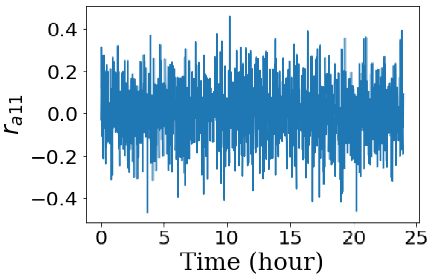
Each residual is sensitive to a set of faults, and the set of residuals for each subsystem can detect all the globally-detectable faults and isolate all the globally-isolable faults in the subsystem. For example, in (18) is sensitive to and and, therefore, can be used to detect these faults. In realistic situations, sensor noise and model uncertainties can have a negative impact on each diagnoser’s performance. For example, consider the case where each sensor in the ADAPT-Lite system has an additive noise with a normal distribution, . Figure 12 shows that because of noise, residual is not zero even when there is no fault in the system.
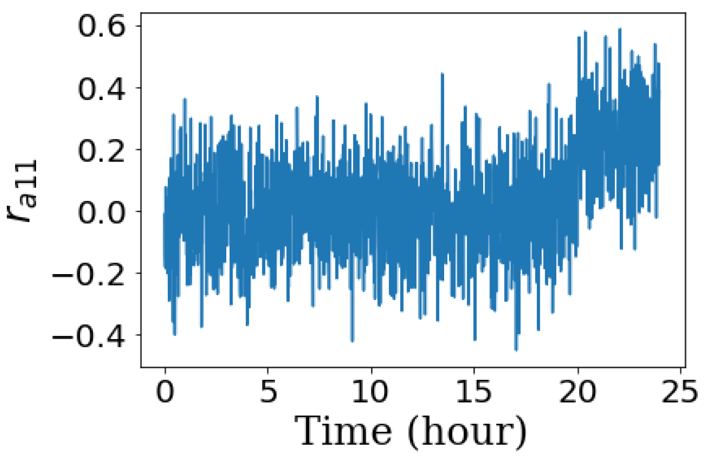
This can impact fault diagnosis performance negatively by increasing false positive rates. Moreover, noise can hide the effect of faults on the residuals and lead to high false negative rates. Figure 13 shows residual when an additive fault 0.25 occurs at 20 h. Sensor noise conceals the fault signal and makes fault detection and isolation more challenging.
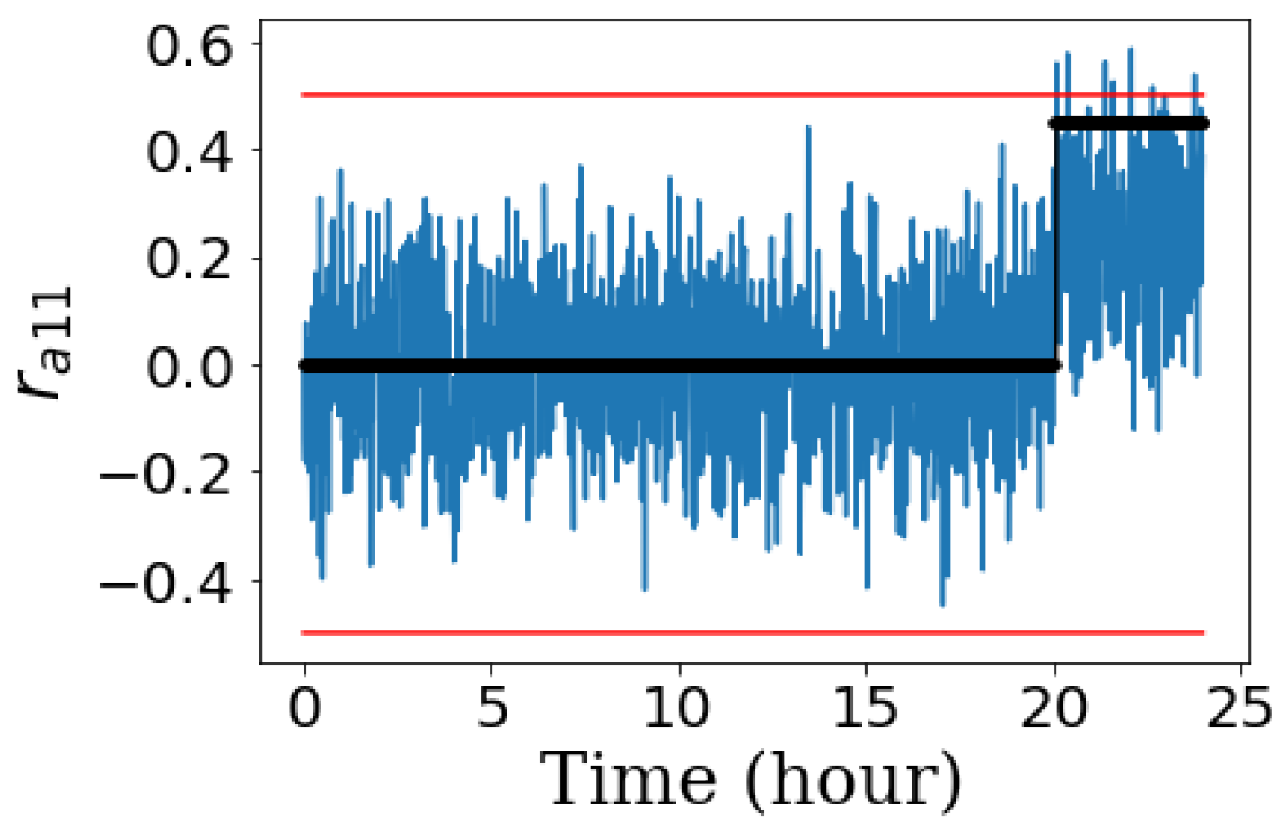
To achieve acceptable performance in practice, it is necessary to design a set of hypothesis tests, such as the Z-test [31], to distinguish faults from noise and uncertainty and determine what residual outputs are significant enough to reject the normal operation assumption and trigger the alarms. Figure 14 shows that a simple hypothesis test can achieve a zero false positive rate and detect in less than 5 min using residual .
5.4. Discussion
The two proposed algorithms for designing distributed diagnosis systems provide a solution with maximum possible detectability and isolability that can be achieved for a system given a set of measurements. Unlike previous work, such as [14,15], our proposed methods were based on system models expressed as equations and, therefore, did not need to use the temporal response and event ordering in the diagnosis, all of which are derived properties and, therefore, require additional computation. Using a purely structural approach reduced the overall diagnosability of the system for the given set of measurements. However, it also reduced the number of assumptions we needed to make about the fault characteristics, such as the order of events in the diagnoses subsystems (which can be error-prone), and we did not have to analyze in detail the subsystem dynamics.
The total number of MSO sets was exponential in terms of the system measurements, and the MSO set selection was equivalent to the set covering problem. Therefore, the MSO-based algorithm had high computational cost especially for large-scale systems. The algorithm guaranteed that the subsystems shared a minimum number of measurements between the subsystems, implying that we minimized the communication of measurement streams across subsystems of the global system. This is important because sending data between subsystems is costly in large-scale systems. Moreover, it is straight forward to extend the MSO-based approach to robust distributed diagnosis by considering residuals’ robustness performance in the selection process [32,33].
The equation-based algorithm found a minimal set of equations from neighboring subsystems that guaranteed the maximum possible detectability and isolability that can be achieved for the system given a set of measurements. The number of equations was significantly smaller than the number of MSO sets. Therefore, the second algorithm was computationally more efficient. Moreover, the second algorithm did not need to use the global model in the design process of the supervisory system. This makes the algorithm very feasible for large-scale complex systems. However, it did not guarantee that the number of shared variables among the subsystems was globally minimum.
6. Conclusions
Two algorithms are proposed for designing distributed diagnosers where the number of sensor data shared between different local diagnosers is minimized. The first method generates the MSO sets for the given global system and selects a subset for each subsystem with minimum required shared variables. Having all the MSO sets computed in advance makes robustness analysis possible for robust distributed MSO set selection. The second algorithm used a heuristic equation-based approach, which is computationally more efficient and makes it suitable for large-scale systems. The ADAPT system case study was used to compare the two algorithms and illustrate the advantages of each method. In future work, we will consider noise and uncertainty in the design step and will extend the distributed diagnosis design problem to robust distributed fault detection and isolation using different methods for decoupling noise and uncertainties.
Author Contributions
The work reported in this paper was a part of the PhD dissertation of H.K. supervised by G.B. at Vanderbilt University. H.K. was the primary developers of the algorithms and he ran the experimental studies with support from G.B. (development, verification) and D.J. (MSO algorithms) from Linköping University. The text of this paper is primarily written by H.K., with organizational and editorial support provided by G.B. D.J. also reviewed and edited the manuscript. All authors also helped with the revisions and edited the final manuscript during the review process.
Funding
This work was partially supported by NASA STTR grant # NNX15CA11C to Vanderbilt University.
Conflicts of Interest
The authors declare no conflict of interest.
References
- Chen, J.; Patton, R.J. Robust Model-Based Fault Diagnosis for Dynamic Systems; Springer Science & Business Media: New York, NY, USA, 2012; Volume 3. [Google Scholar]
- Blanke, M.; Kinnaert, M.; Lunze, J.; Staroswiecki, M. Diagnosis and Fault-Tolerant Control; Springer: New York, NY, USA, 2015. [Google Scholar]
- Duarte, E.P., Jr.; Nanya, T. A hierarchical adaptive distributed system-level diagnosis algorithm. IEEE Trans. Comput. 1998, 47, 34–45. [Google Scholar] [CrossRef]
- Spitzer, C. Honeywell primus epic aircraft diagnostic and maintenance. In Digital Avionics Handbook; CRC Press Book: Boca Raton, FL, USA, 2007; pp. 22–23. [Google Scholar]
- Aslin, M.J.; Patton, G.J. Central Maintenance Computer System and Fault Data Handling Method. U.S. Patent 4 943 919, 24 July 1990. [Google Scholar]
- Lanigan, P.E.; Kavulya, S.; Narasimhan, P. Diagnosis in Automotive Systems: A Survey; Technical Report CMU-PDL-11-110; Carnegie Mellon University PDL: Pittsburgh, PA, USA, 2011. [Google Scholar]
- Ferrari, R.M.; Parisini, T.; Polycarpou, M.M. Distributed fault detection and isolation of large-scale discrete- time nonlinear systems: An adaptive approximation approach. IEEE Trans. Autom. Control 2012, 57, 275–290. [Google Scholar] [CrossRef]
- Ruiz, L.B.; Siqueira, I.; Oliveira, L.B.; Wong, H.C.; Nogueira, J.M.S.; Loureiro, A.A.F. Fault management in event-driven wireless sensor networks. In Proceedings of the MSWiM’04, Venezia, Italy, 4–6 October 2004. [Google Scholar]
- Rish, I.; Brodie, M.; Ma, S.; Odintsova, N.; Beygelzimer, A.; Grabarnik, G.; Hernandez, K. Adaptive diagnosis in distributed systems. IEEE Trans. Neural Netw. 2005, 16, 1088–1109. [Google Scholar] [CrossRef] [PubMed]
- Shames, I.; Teixeira, A.M.; Sandberg, H.; Johansson, K.H. Distributed fault detection for interconnected second-order systems. Automatica 2011, 47, 2757–2764. [Google Scholar] [CrossRef]
- Boem, F.; Ferrari, R.M.; Keliris, C.; Parisini, T.; Polycarpou, M.M. A distributed networked approach for fault detection of large-scale systems. IEEE Trans. Autom. Control 2017, 62, 18–33. [Google Scholar] [CrossRef]
- Chanthery, E.; Travé-Massuyès, L.; Indra, S. Fault isolation on request based on decentralized residual generation. IEEE Trans. Syst. Man Cybern. Syst. 2016, 46, 598–610. [Google Scholar] [CrossRef]
- Roychoudhury, I.; Biswas, G.; Koutsoukos, X. Designing distributed diagnosers for complex continuous systems. IEEE Trans. Autom. Sci. Eng. 2009, 6, 277–290. [Google Scholar] [CrossRef]
- Daigle, M.J.; Koutsoukos, X.D.; Biswas, G. Distributed diagnosis in formations of mobile robots. IEEE Trans. Robot. 2007, 23, 353–369. [Google Scholar] [CrossRef]
- Bregon, A.; Daigle, M.; Roychoudhury, I.; Biswas, G.; Koutsoukos, X.; Pulido, B. An event-based distributed diagnosis framework using structural model decomposition. Artif. Intell. 2014, 210, 1–35. [Google Scholar] [CrossRef]
- Ferrari, R.M.; Parisini, T.; Polycarpou, M.M. Distributed fault diagnosis with overlapping decompositions: An adaptive approximation approach. IEEE Trans. Autom. Control 2009, 54, 794–799. [Google Scholar] [CrossRef]
- Khorasgani, H.; Biswas, G.; Jung, D.E. Minimal Structurally Overdetermined Sets Selection for Distributed Fault Detection. In Proceedings of the International Workshop on Principles of Diagnosis (DX-15), Paris, France, 31 August–3 September 2015. [Google Scholar]
- Khorasgani, H.; Jung, D.E.; Biswas, G. Structural approach for distributed fault detection and isolation. IFAC-PapersOnLine 2015, 48, 72–77. [Google Scholar] [CrossRef]
- Daigle, M.J.; Roychoudhury, I.; Biswas, G.; Koutsoukos, X.D.; Patterson-Hine, A.; Poll, S. A comprehensive diagnosis methodology for complex hybrid systems: A case study on spacecraft power distribution systems. IEEE Trans. Syst. Man Cybern. Part A Syst. Hum. 2010, 5, 917–931. [Google Scholar] [CrossRef]
- Krysander, M.; Åslund, J.; Nyberg, M. An efficient algorithm for finding minimal overconstrained subsystems for model-based diagnosis. IEEE Trans. Syst. Man Cybern. Part A Syst. Hum. 2008, 38, 197–206. [Google Scholar] [CrossRef]
- Rosich, A.; Frisk, E.; Aslund, J.; Sarrate, R.; Nejjari, F. Fault diagnosis based on causal computations. IEEE Trans. Syst. Man Cybern. Part A Syst. Hum. 2012, 42, 371–381. [Google Scholar] [CrossRef]
- Frisk, E.; Krysander, M.; Jung, D. A Toolbox for Analysis and Design of Model Based Diagnosis Systems for Large Scale Models. In Proceedings of the IFAC World Congress, Toulouse, France, 21 April 2017. [Google Scholar]
- Nejjari, F.; Sarrate, R.; Rosich, A. Optimal sensor placement for fuel cell system diagnosis using bilp formulation. In Proceedings of the 2010 18th Mediterranean Conference on Control & Automation (MED), Marrakech, Morocco, 23–26 June 2010; pp. 1296–1301. [Google Scholar]
- Wolsey, L.A.; Nemhauser, G.L. Integer and Combinatorial Optimization; John Wiley and Sons: New York, NY, USA, 2014. [Google Scholar]
- Land, A.H.; Doig, A.G. An Automatic Method of Solving Discrete Programming Problems. Econom. J. Econom. Soc. 1960, 497–520. [Google Scholar] [CrossRef]
- Mitchell, J.E. Branch-and-Cut Algorithms for Combinatorial Optimization Problems. In Handbook of Applied Optimization; Oxford University Press: Oxford, UK, 2002; pp. 65–77. [Google Scholar]
- Flaugergues, V.; Cocquempot, V.; Bayart, M.; Pengov, M. Structural Analysis for FDI: A modified, invertibility-based canonical decomposition. In Proceedings of the 20th International Workshop on Principles of Diagnosis, DX09, Warsaw, Poland, 27–30 August 2009; pp. 59–66. [Google Scholar]
- Khorasgani, H.; Biswas, G. Structural Fault Detection and Isolation in Hybrid Systems. IEEE Trans. Autom. Sci. Eng. 2017, 15, 1585–1599. [Google Scholar] [CrossRef]
- Armengol, J.; Bregón, A.; Escobet, T.; Gelso, E.; Krysander, M.; Nyberg, M.; Olive, X.; Pulido, B.; Travé-Massuyès, L. Minimal Structurally Overdetermined sets for residual generation: A comparison of alternative approaches. In Proceedings of the 7th IFAC Symposium on Fault Detection, Supervision and Safety of Technical Processes, SAFEPROCESS09, Beijing, China, 2–4 September 2009. [Google Scholar]
- Daigle, M.J.; Roychoudhury, I.; Bregon, A. Qualitative event-based diagnosis applied to a spacecraft electrical power distribution system. Control Eng. Pract. 2015, 38, 75–91. [Google Scholar] [CrossRef]
- Biswas, G.; Simon, G.; Mahadevan, N.; Narasimhan, S.; Ramirez, J.; Karsai, G. A robust method for hybrid diagnosis of complex systems. In Proceedings of the 5th Symposium on Fault Detection, Supervision and Safety for Technical Processes, Washington, DC, USA, 9–11 June 2003; pp. 1125–1131. [Google Scholar]
- Khorasgani, H.; Jung, D.E.; Biswas, G.; Frisk, E.; Krysander, M. Robust Residual Selection for Fault Detection. In Proceedings of the IEEE 53rd Annual Conference on Decision and Control (CDC), Melbourne, Australia, 12–15 December 2014. [Google Scholar]
- Khorasgani, H.; Jung, D.E.; Biswas, G.; Frisk, E.; Krysander, M. Off-line robust residual selection using sensitivity analysis. In Proceedings of the International Workshop on Principles of Diagnosis (DX-14), Graz, Austria, 8–11 September 2014. [Google Scholar]
Figure 1.
Running example: four-tank system.

Figure 2.
Dulmage–Mendelsohn (DM) decomposition of the first subsystem model.

Figure 3.
DM decomposition of .

Figure 4.
DM decomposition of .

Figure 5.
DM decomposition of .

Figure 6.
Finding the minimal sets of equations in to compute .

Figure 7.
DM decomposition of .

Figure 8.
DM decomposition of .

Figure 9.
DM decomposition of .

Figure 10.
Expanding the search environment to the higher order connected subsystems.

Figure 11.
ADAPT-Lite subsystems [30]. CB, Circuit Breaker.
Figure 11.
ADAPT-Lite subsystems [30]. CB, Circuit Breaker.

Figure 12.
Residual for 24 h when each sensor in the ADAPT-Lite system has an additive noise with a normal distribution, , and the system is in normal operation.
Figure 12.
Residual for 24 h when each sensor in the ADAPT-Lite system has an additive noise with a normal distribution, , and the system is in normal operation.

Figure 13.
Residual for 24 h when each sensor in the ADAPT-Lite system has an additive noise with a normal distribution, , and 0.25 occurs at h.
Figure 13.
Residual for 24 h when each sensor in the ADAPT-Lite system has an additive noise with a normal distribution, , and 0.25 occurs at h.

Figure 14.
A hypothesis test can achieve a zero false positive rate and detect in :48″ using residual . The step function represents the detection time.
Figure 14.
A hypothesis test can achieve a zero false positive rate and detect in :48″ using residual . The step function represents the detection time.


Table 1.
Set of augmented measurements for each subsystem model.
| Subsystem | Set of Augmented Measurements |
|---|---|
| , , | |
| , | |
Table 2.
Set of augmented constraints and measurements for each subsystem model.
| Subsystem | Augmented Equations | Augmented Measurements |
|---|---|---|
| , , , , | , , | |
| , , , | , | |
Table 3.
Set of augmented measurements for each ADAPT subsystem using the global method.
| Subsystem | Set of Augmented Measurements |
|---|---|
| Subsystem 1 | - |
| Subsystem 2 | |
| Subsystem 3 | |
| Subsystem 4 | |
| Subsystem 5 |
Table 4.
Set of Minimal Structurally-Over-determined (MSO) sets for each local diagnoser using the MSO-based method.
Table 4.
Set of Minimal Structurally-Over-determined (MSO) sets for each local diagnoser using the MSO-based method.
| Subsystem | Set of MSO Sets |
|---|---|
| 1 | |
| 2 | |
| 3 | |
| 4 | |
| 5 |
Table 5.
Set of augmented equations and measurements for each subsystem model using the equation- based approach.
Table 5.
Set of augmented equations and measurements for each subsystem model using the equation- based approach.
| Subsystem | Augmented Equations | Augmented Measurements |
|---|---|---|
| Subsystem 1 | - | - |
| Subsystem 2 | , , , , | |
| Subsystem 3 | ||
| Subsystem 4 | , , | |
| Subsystem 5 |
Table 6.
Set of MSO sets for each local diagnoser using the equation-based approach.
| Subsystem | Set of MSO Sets |
|---|---|
| 1 | |
| 2 | |
| 3 | |
| 4 | , , |
| 5 |
© 2019 by the authors. Licensee MDPI, Basel, Switzerland. This article is an open access article distributed under the terms and conditions of the Creative Commons Attribution (CC BY) license (http://creativecommons.org/licenses/by/4.0/).
Share and Cite
MDPI and ACS Style
Khorasgani, H.; Biswas, G.; Jung, D. Structural Methodologies for Distributed Fault Detection and Isolation. Appl. Sci. 2019, 9, 1286. https://doi.org/10.3390/app9071286
AMA Style
Khorasgani H, Biswas G, Jung D. Structural Methodologies for Distributed Fault Detection and Isolation. Applied Sciences. 2019; 9(7):1286. https://doi.org/10.3390/app9071286
Chicago/Turabian StyleKhorasgani, Hamed, Gautam Biswas, and Daniel Jung. 2019. "Structural Methodologies for Distributed Fault Detection and Isolation" Applied Sciences 9, no. 7: 1286. https://doi.org/10.3390/app9071286
Note that from the first issue of 2016, this journal uses article numbers instead of page numbers. See further details here.