Active Control of Broadband Noise Inside a Car Using a Causal Optimal Controller

College of Power and Energy Engineering, Harbin Engineering University, Harbin 150001, China
*
Author to whom correspondence should be addressed.
Appl. Sci. 2019, 9(8), 1531; https://doi.org/10.3390/app9081531
Submission received: 8 March 2019
/
Revised: 7 April 2019
/
Accepted: 8 April 2019
/
Published: 12 April 2019
(This article belongs to the Special Issue Active and Passive Noise Control)
Abstract
:This paper investigates active broadband noise control inside vehicles with a multichannel controller. The noncausal inversion of a practical nonminimum-phase secondary path is formulated, and its influence on noise-reduction performance is analyzed. Based on multiple coherence between reference signals and undesired noise, a novel formulation for identifying primary paths with correlated excitation signals is presented and a causal optimal controller is proposed. Meanwhile, the proposed controller can be used as an accurate predictor to estimate the maximal achievable noise reduction and provide a reference to improve the control systems. The robustness of the proposed algorithm is examined by varying the uncertainty of primary paths. Finally, the performance of the proposed causal optimal controller is validated using the data measured in a car. The results show that the proposed algorithm outperforms traditional algorithms and achieves a significant broadband noise reduction in time-invariant systems.
1. Introduction
The acoustic quality of a car determines its ride comfort and has been a significant marketing issue for car manufacturers [1]. Broadband road noise inside a car, caused by road-tyre interaction, is the main noise source when a car is driving at a relatively high speed [2]. Thus, measures have to be taken to isolate or reduce this noise to an acceptable level. Traditionally, sound-absorbing materials have been used to attenuate the noise. However, when they are used to reduce low-frequency noise, the mass and space they require can be out of scale. In order to overcome this problem, the active control system is applied [3].
Active control of the interior road noise of a car has been researched for over two decades, and a variety of active noise control (ANC) techniques have been proposed to improve ride comfort [4,5,6]. Sutton et al. proved that at least six vibrational reference signals are required to attenuate broadband road noise by using a filtered-x least mean square (FXLMS) algorithm [4]. Sano et al. used a H∞ controller to cancel the noise around front seat, although only a reduction of 10 dB at 40 Hz was achieved [7]. Oh et al. proposed a leaky constraint multiple FXLMS algorithm, and road-booming noise around 250 Hz was reduced about 6 dB at the error microphone positions [8]. Belgacem et al. used an active structural acoustic control technique to reduce the vibration of suspensions, and a 4.6 dB attenuation was measured in the 50–250 Hz on a quarter-car test bench [9]. Cheer and Elliott show that a multi-input multi-output system was required to have a distinct reduction for the broadband noise [10,11]. Further, Jung et al. used a headrest system to reduce interior road noise around a listener’s ears with remote microphone technique [12]. Although many algorithms were explored, the constraints limiting the improvement of control performance for broadband road noise still have not been solved [9,13].
As we know, the performance of ANC systems relies heavily on the secondary path characteristics [14]. To improve control results, high modelling accuracy of the secondary path is required [15,16]. However, if the secondary path is a nonminimum-phase system, it will generate a waterbed effect on the control system, which has a significant influence on the design of the controller and the deterioration of the control performance [13,17], regardless of the fact that the controller is designed by FXLMS [18] or H∞ robust control algorithms [19]. Under this situation, even a perfect modelling cannot lead to a satisfactory result [20]. Although the above adaptive control algorithms have the ability to reduce noise with time-varying primary paths, the best control results cannot be achieved due to their large gradient estimation deviation of the cost fuction for time-varying noise.
In this paper, a novel formulation for identifying primary paths with correlated excitation signals is presented, and the influence of a nonminimum-phase secondary path on the control system is investigated. Based on the theoretical analysis, a novel causal optimal controller is proposed to improve the control performance for the time-invariant system. Besides, the traditional method to predict the noise reduction is using the coherence between reference and noise signals [4,11,21]. The resulting prediction has a large deviation from the practical reduction, because it does not take causality constraint into account. Since the proposed controller considers the nonminimum-phase characteristics of secondary paths as well as the frequency responses of systems, it can also be used as a more accurate predictor to estimate the maximal achievable noise reduction and is more instructive in engineering. All the work is conducted under the assumption that the control systems are linear time-invariant.
The organisation of this paper is as follows. In Section 2, the impact of a nonminimum-phase secondary path on the noise-reduction performance is analysed and its noncausal inversion is formulated. Section 3 presents a novel formulation for the identification of multiple primary paths with correlated excitation signals, and a causal optimal controller is proposed. In Section 4, the robustness and computational complexity of proposed algorithm is examined and control performance is validated. Conclusions are provided in Section 5.
2. Secondary Path Analysis
2.1. Influence of a Secondary Path on Control Performance
The block diagram of a control system is shown in Figure 1, where z = ej2πf, P(z) and S(z) correspond to the primary and secondary paths, W(z) is the controller, and d(n) and (n) represent the undesired noise and output signal of the control system, respectively. If the output signal is designed to cancel the undesired noise completely, the resulting optimal controller W(z) will have the following expression:
Apparently, the optimal controller is a result of the convoluting transfer functions of the primary path and the inversion of the secondary path. Unfortunately, most of the secondary paths in the engineering are nonminimum-phase and their inversions may be unstable [20]. To circumvent the problem, we expand the inversion of S(z) as a noncausal filter and use a causal filter C(z) to approximate it as [22], as follows:
where z−D denotes D sampling times delay. Thus, the optimal controller can be rewritten as Wopt(z) = zDC(z)P(z). It is assumed that H(z) = P(z)C(z) and the impulse response of H(z) is hn, n = 0,···,Nh−1; then, the optimal output signal of the controller Wopt(z) is [20], as follows:
where n denotes current sampling time. If n + D − i < n, it means x(n + D − i) is a past input signal. Similarly, if n + D − i > n, it means x(n + D − i) is a future input signal. It can be seen from above equation that the first part of the optimal output signal yopt(n) is a linear convolution of the future input signal with the system impulse response hn and the second part is a convolution of the past input signal with the impulse response hn. For the controller W(z), the second part of the optimal output signal can be generated by using the past input signal and causal part of system response. However, to produce the first part of the optimal output signal, it needs the future input signal, which is impossible for the controller to obtain. Therefore, the best noise-reduction performance, which is achievable for a physical system, can be derived by designing a controller with the causal part of the system impulse response.
2.2. Noncausal Inversion
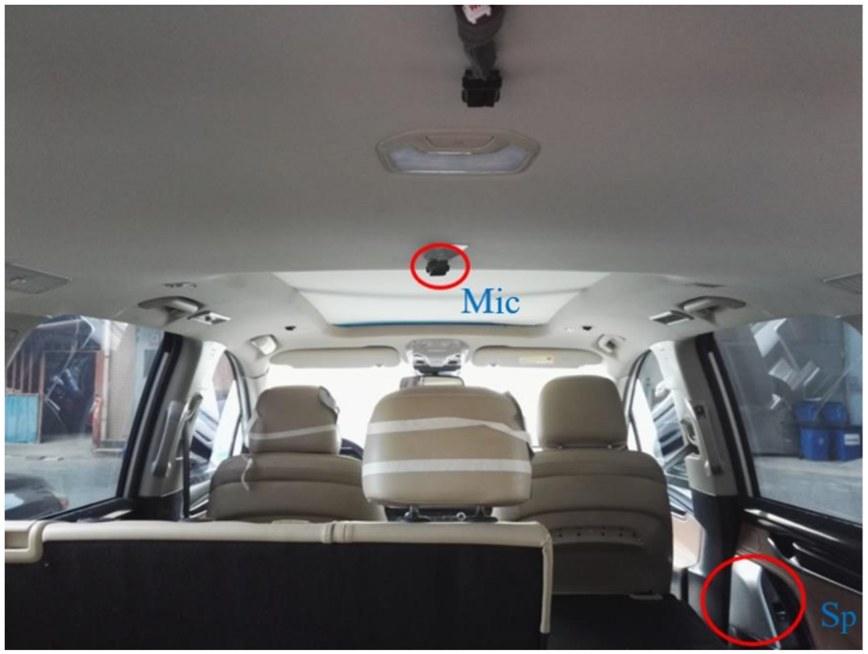
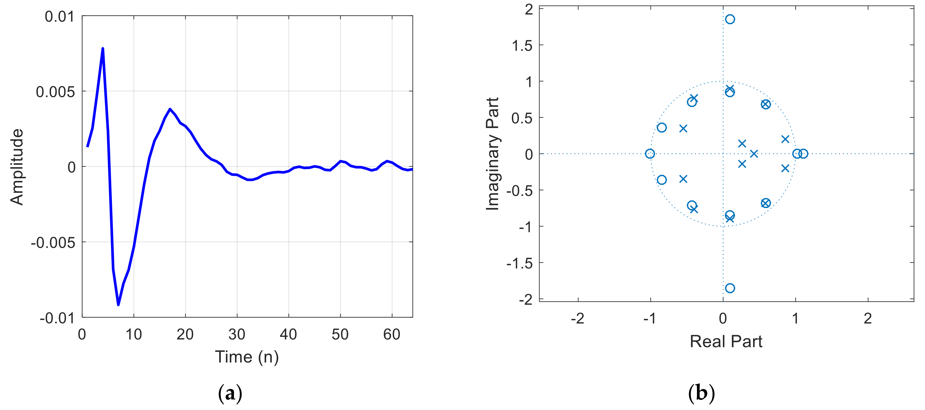
In this part, a practical secondary path shown in Figure 2 is adopted, where Sp and Mic denote the door loudspeaker and error microphone, respectively. The secondary path from the output of the controller to the measured signal of Mic is identified with a 13th order infinite impulse response (IIR) filter and its impulse response, zeros, and poles distribution are shown in Figure 3. It can be seen from Figure 3b that there are five zeros outside the unit circle. Thus, the secondary path is a nonminimum-phase system, and its inversion will contain both causal and noncausal parts.
From Figure 3b, we know that there are no repeated zeros in the secondary path. So, its inversion S−1(z) can be expressed using partial fraction decomposition as [23], as follows:
where pq is the qth pole of S−1(z) and also the qth zero of S(z) and Aq is the related coefficient. Because all the coefficients of the filter S(z) are real, its poles and zeros must be either purely real or appear in complex conjugate pairs. By including the unit circle into the convergence region, the term Aq/(1 − pqz−1) of Equation (4) corresponding to purely real pq can be expanded as follows:
For a pair of conjugate zeros pq and of S(z), their corresponding coefficients are also conjugate. Thus, the expansions can be simplified from Equation (5) into an expression of conjugate pairs. According to whether the conjugate zeros pair, pq and , are inside or outside the unit circle; their expansion (z) can be rewritten as Equations (6), as follows:
where αq, βq, and rq are derived from , . Equation (6) corresponds to the causal and noncausal responses of conjugate zeros pairs. By substituting Equations (5) and (6) for Equation (4), the inversion of S(z) is obtained as follows:
The finite impulse response of S−1(z) in Equation (7) corresponding to the secondary path in Figure 2 is shown in Figure 4. The noncausal part of the response is displayed in the range of [−400, 0), which is the summation of Equation (7) when |pq| > 1. The causal part of the response is shown in the range of [0, 100], which is the summation of Equation (7) when |pq| ≤ 1. It can be seen that it will take a long period for noncausal response to decay. Therefore, the nonminimum-phase secondary path S(z) will have a significant effect on control performance, and a large proportion of the undesired noise cannot be reduced using this secondary path.
3. Formulation of the Causal Optimal Controller
Since broadband road noise inside a car is produced by the interaction between road surface and tires, it is complicated and at least six reference signals are required to achieve a satisfactory result [5]. Therefore, the combination of reference signals needs to be chosen according to coherence function between input signal x(n) and output undesired noise d(n) [24]. Since the vibrational signals measured in a vehicle are correlative to each other, the multiple coherence cannot be calculated directly, and the partial coherence function is required, which is defined as follows:
where , , and are the residual power spectral density functions and the residual cross-spectral density function of signals xk, d after removing the components relating to the signals x1···xk−1 at frequency f. When k = 1, they are simplified as , , and , which can be derived from the autocorrelation and cross-correlation functions using discrete Fourier transformation [23]. The residual spectral density function can be derived using the following expression:
where i and j denote the signals xk or d.
The partial coherence function of Equation (8) represents the contribution of signal xk to the power of signal d after removing signals x1···xk−1 from them. Once they are acquired, the multiple coherence between reference signals x1···xK and the undesired noise d can be derived as follows [24]:
The result of Equation (10) represents the multiple coherence between the undesired noise and the set of reference signals. As we know, a widely accepted expression to estimate the maximal noise reduction is [4,11,21], as follows:
The above equation shows that the larger the result of Equation (10), the more potential noise reduction can be achieved. Thus, the most appropriate reference signals can be obtained according to the calculation results of all the different combinations of K signals from all the measured vibrational signals. The combination of K signals with the largest multiple coherence value will be used as reference signals, and the corresponding primary paths of vibration and noise propagation are required to be identified. Since the disturbances in the input and output signals cannot be acquired, it is appropriate to assume that their power ratio equals one and identify the primary system paths using the following equation [25]:
The first primary path can be identified directly using Equation (12). For modelling the kth (k > 1) primary path, however, we need to remove the components related to the former k − 1 reference signals from the signal and undesired noise d. Similarly, using residual power spectral density and residual cross-spectral density functions and , and and derived from Equation (9), the kth primary path can be identified as follows:
Transforming Equation (13) into z domain and substituting the result and Equation (7) into Equation (1), the optimal controller can be expressed as follows:
As is explained in Section 2.1 and Figure 4, the future reference signals of an ANC system cannot be acquired. Thus, the noncausal part of the optimal controller has to be discarded, and the causal optimal controller (COC) is derived as follows:
where the subscript + denotes the causal part of the optimal controller, that is, the terms with non-positive exponential index of z. Equation (15) is a causal optimal controller for a physical system, and the best noise-reduction result can be achieved with it. Meanwhile, Equation (15) can also be used to predict the achievable noise-reduction performance by transforming it into frequency domain and substituting it for the following expression:
Equation (11) is a widely accepted expression to predict the noise reduction by considering the coherence between reference and noise signals. However, the predicted performance is difficult to achieve in the engineering since it does not take causality constraint into account. In practice, due to the limitation of the nonminimum-phase characteristics of secondary paths, the achievable noise reduction is far less than the predicted result of Equation (11). For the predicted result using Equation (16), since it considers the nonminimum-phase characteristics of secondary paths as well as the frequency responses of primary and secondary paths, the result is the maximal noise reduction that a physical system can be achieved and is more instructive in engineering. Thus, equation (11) is more suitable to be a criterion for selecting reference signals, while Equation (16) is more appropriate to be a predictor for estimating the control results.
4. Algorithm Verification and Discussion
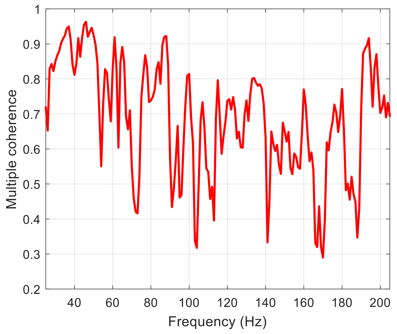
The proposed causal optimal controller in Equation (15) is verified in this section using the data measured from a car driving at 60 km/h in third gear with a sampling frequency of 1600 Hz. The positions of the loudspeaker and error microphone are shown in Figure 2. Vibrational signals of the car are adopted as reference signals, and they are acquired by installing eight triaxial accelerometers on the chassis of the car. The positions of accelerometers are shown in Figure 5, where ACC1—ACC8 represent eight triaxial accelerometers, and Mic and Sp represent the error microphone and door loudspeaker. Due to the distance limitation between the error microphone and ears, only the noise below 200 Hz is expected to be cancelled.
Six reference signals are selected from twenty-four vibrational signals according to the multiple coherence results, and they are ACC2-X, ACC2-Z, ACC4-X, ACC6-X, ACC6-Y, and ACC7-Y. The multiple coherence between the selected reference signals and the undesired noise is shown in Figure 6. It can be observed that the average of the multiple coherence between 30 and 200 Hz is over 0.6. Therefore, the reference signals are acceptable.
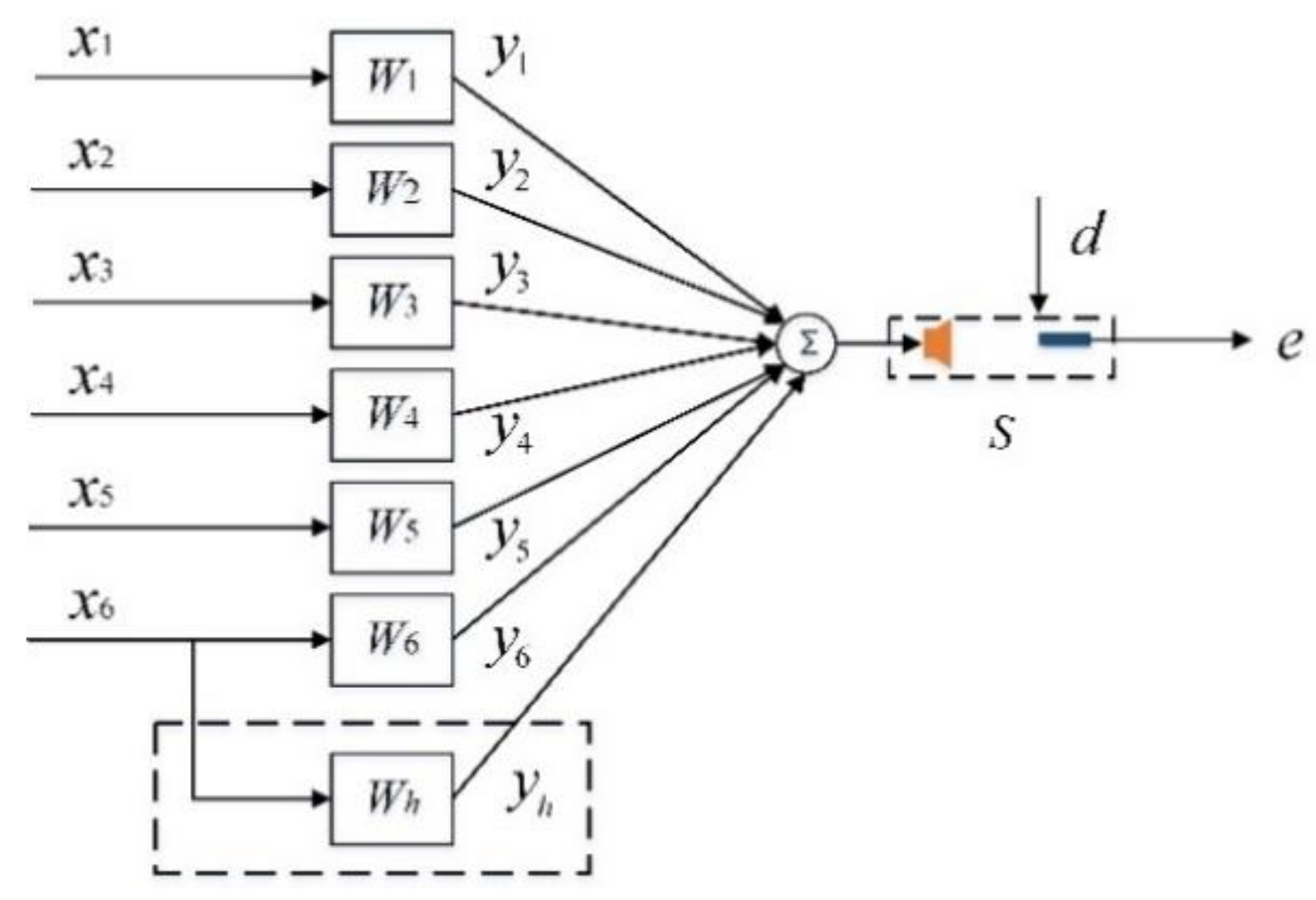
Based on above analysis, a multichannel control system is designed as is shown in Figure 7, where xi and Wi, i = 1,⋯,6 denote six reference signals and controllers, respectively. Each controller Wi has the expression as Equation (15). If only the broadband noise is going to be cancelled, using six proposed causal optimal controllers can achieve a satisfactory result. If the broadband as well as engine harmonic noises are expected to be reduced, it is appropriate to add an adaptive controller Wh into the control system to cancel the harmonic component. The design of Wh is based on FXLMS algorithm, and the adopted reference signal should include the engine harmonics [26].
A six-channel FXLMS algorithm is also adopted here for performance comparison. The resultant error signal of the algorithm is derived as follows:
where * denotes convolution and s(n) is the impulse response of the secondary path S, which is identified offline in advance [26]. By taking the square of the instantaneous error e(n) as a cost function, the updating equation for each adaptive filter of FXLMS algorithm is obtained [26] as follows:
where µ is the step size for updating the control filter; δ is a normalization constant; and xif(n) is the ith filtered reference signal vector, which is the convolution result of the ith reference signal and the secondary path s(n).
The noise reduction is evaluated using the parameter Rd, which is defined as follows:
4.1. Robustness and Computational Complexity Analysis
In practice, the real primary path of a physical system may vary from the identified result . Thus, the robustness of the proposed control algorithm has to be examined by defining the uncertainty of the primary path as follows:
where ‖ ‖∞ denotes the infinite norm of the expression.
The control performances are evaluated under different uncertainties. In the examination, six primary paths P1,⋯,P6 are identified using the method proposed in Section 3, and six broadband random noise signals are applied to the real primary paths as excitation sources to produce a noise signal, where the real primary paths , k = 1,⋯,6 are derived as according to different uncertainties Δ, and V is a normalized random signal vector with maximal amplitude of one. Meanwhile, six causal optimal controllers derived using the identified primary paths P1,⋯,P6 are adopted as controllers. Since the coefficients of the proposed COC controller approximate zero when its length is larger than 768, each filter of proposed COC algorithm and FXLMS algorithm is selected with the same memory length of 768. For the FXLMS algorithm, the step size and normalization constant are µ = 0.1, δ = 0.1. Under a specific uncertainty Δ, a random signal vector V is generated to obtain the different real primary paths , k = 1,⋯,6. The simulation results of averaging 50 independent runs for each specific uncertainty Δ are displayed in Figure 8. FXLMS algorithm is adaptive, and it can adjust its coefficients to different primary paths. Therefore, the control results of FXLMS algorithm for different primary paths are similar, and only the result with uncertainty Δ = 0 is shown in Figure 8.
It can be observed from Figure 8 that the nominal noise reduction of proposed COC (Δ = 0) is about 8 dB, and by increasing uncertainty Δ to 300%, the corresponding noise reduction decreases to 3 dB, which is at the same level as the result of FXLMS algorithm. Therefore, the proposed method can achieve better noise-reduction performance if the modelling accuracy of primary paths is within 300%. In most of cases, the modelling uncertainty can be limited within this range. Thus, the modelling errors of primary paths do not significantly deteriorate the noise-reduction performance, and the results of proposed algorithm are better than that of FXLMS algorithm. It should be noted that even though all the undesired noise is caused by the reference signals, only a small reduction is obtained. This is because the results are deteriorated by the nonminimum-phase characteristics of the secondary path.
The computational complexity of the proposed COC algorithm and FXLMS algorithm is shown in Table 1, where L, N, M denote the length of the control filter, the secondary path, and the number of channels; ± and × denote the manipulations of addition and subtraction, and multiplication, respectively. Compared with the FXLMS algorithm, the proposed COC algorithm requires less computation irrespective of cancelling broadband noise or broadband as well as harmonic noises. Its advantage becomes more significant when the number of channels M is increased.
4.2. Implementation and Verification
In this subsection, the simulations are performed using the data measured from the setup of Figure 2 and Figure 5 when the car is driving at a rough road. Since the noise inside a car contains both broadband noise and harmonics of the engine, an adaptive controller Wh updated using FXLMS algorithm is added into the control system to reduce the engine harmonic noise, and the proposed six-channel causal optimal controllers are used to reduce the broadband noise. The parameters for COC and FXLMS algorithms are L = 768, µ = 0.002, and δ = 0.1.
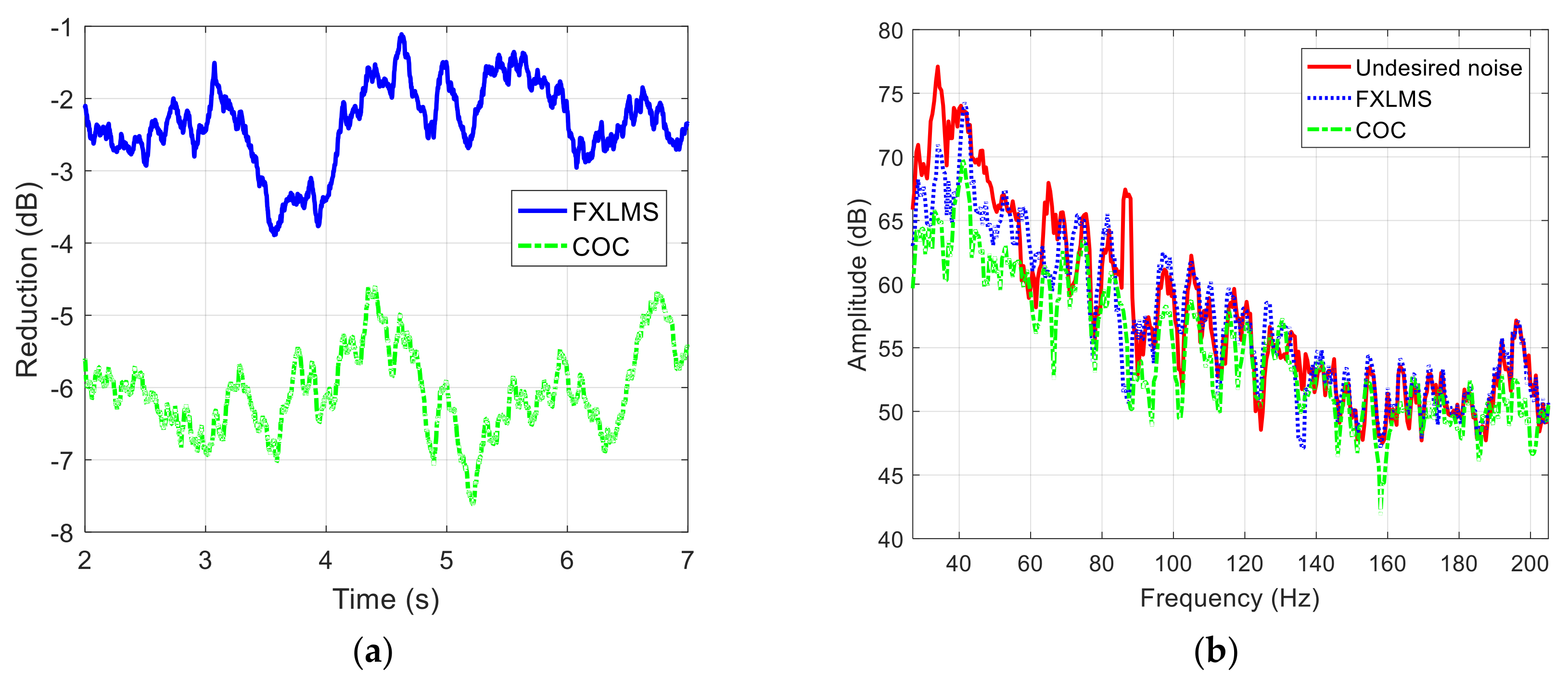
The control results in time domain are shown in Figure 9a. It can be seen that the proposed COC algorithm outperforms FXLMS algorithm with an approximate 6 dB reduction, while FXLMS algorithm only obtains a 2.5 dB noise reduction. Comparing Figure 9a with Figure 8, we can find that the noise reductions of two algorithms are decreased. That is because all the undesired noise in Figure 8 is caused by the six reference signals, while for the noise inside a car, only part of it is induced by the reference signals. Thus, the control performance can be improved further by increasing the number of reference signals.
The control results in frequency domain are shown in Figure 9b. The main attenuation occurs around 34 and 87 Hz. The noise peak at 34 Hz is caused by the resonance of the car. After control, FXLMS algorithm achieves about 7 dB reduction at peak, while for the proposed COC algorithm, a maximal reduction up to 12 dB is achieved. The peak at 87 Hz is the second-order harmonic of the engine, which is reduced distinctly under two algorithms. Meanwhile, for the noise between 30 and 130 Hz, the proposed COC algorithm achieves a significant reduction in the whole frequency band. However, FXLMS algorithm only reduces some peaks slightly. This is because the cost function of FXLMS algorithm is the square of the instantaneous error, which leads the FXLMS algorithm to reduce the maximal noise component first (beforehand, the other noise components cannot be attenuated effectively). Besides, FXLMS algorithm is derived by using the instantaneous error e2(n) to replace its expectation E(e2(n)); its gradient estimation deviation may be large, especially under time-varying noise. These factors will deteriorate the control result of FXLMS algorithm.
5. Conclusions
This paper analyzed the achievable noise reduction of a control system with a nonminimum-phase secondary path, and a causal optimal controller (COC) was proposed using the convolution of noncausal inversion of the secondary path and the identification results of primary paths. The proposed causal optimal controller can also be used to predict the noise reduction as a complement of the multiple coherence. Since the causality constraint was considered, the predicted result of the proposed controller is the maximal noise reduction with which a physical control system can be achieved. Thus, it is more instructive in terms of engineering.
The robustness examination showed that the proposed causal optimal controller outperforms the FXLMS algorithm, provided that the uncertainties of the primary paths are within 300%. If the modelling errors of the primary paths are larger than 300%, the control results of the proposed algorithm will deteriorate. The performance of the proposed causal optimal controller was validated using the data measured in a car, and an overall noise reduction of 6 dB was predicted with the assumption that both primary and secondary paths are linear time-invariant. Furthermore, the proposed algorithm achieved a significant reduction in the whole frequency band of 30–130 Hz, and the maximal reduction was found to be up to 12 dB at some peaks.
Author Contributions
Methodology, L.Z. and T.Y.; software and validation, L.P. and M.Z.; formal analysis, X.L. and L.P.; writing—original draft preparation, L.Z. and T.Y.; writing—review and editing, L.Z. and X.L.
Funding
This research was funded by the National Natural Science Foundation of China, No. 51375103.
Acknowledgments
The authors would like to thank Ruixiang Wong of the University of Western Australia for providing language help. This work was supported by Shanghai db Electronic Technology Co., LTD.
Conflicts of Interest
The authors declare no conflict of interest.
References
- Jari, K. Development of A Robust And Computationally-Efficient Active Sound Profiling Algorithm in A Passenger Car: Licentiate Thesis; VTT Technical Research Centre of Finland: Espoo, Finland, 2012. [Google Scholar]
- Forssén, J.; Hoffmann, A.; Kropp, W. Auralization model for the perceptual evaluation of tyre–road noise. Appl. Acoust. 2018, 132, 232–240. [Google Scholar] [CrossRef]
- Kletschkowski, T. Adaptive Feed-Forward Control of Low Frequency Interior Noise; Springer Netherlands: Dordrecht, The Netherlands, 2012. [Google Scholar]
- Sutton, T.J.; Elliott, S.J.; McDonald, A.M.; Saunders, T.J. Active control of road noise inside vehicles. Noise Control Eng. J. 1994, 42. [Google Scholar] [CrossRef]
- Samarasinghe, P.N.; Zhang, W.; Abhayapala, T.D. Recent Advances in Active Noise Control Inside Automobile Cabins: Toward quieter cars. IEEE Signal Processing Magazine 2016, 33, 61–73. [Google Scholar] [CrossRef]
- Wang, Y.S.; Feng, T.P.; Wang, X.L.; Guo, H.; Qi, H.Z. An improved LMS algorithm for active sound-quality control of vehicle interior noise based on auditory masking effect. Mech. Syst. Signal Proc. 2018, 108, 292–303. [Google Scholar] [CrossRef]
- Sano, H.; Inoue, T.; Takahashi, A.; Terai, K.; Nakamura, Y. Active control system for low-frequency road noise combined with an audio system. IEEE Trans. Speech Audio Process. 2001, 9, 755–763. [Google Scholar] [CrossRef]
- Oh, S.H.; Kim, H.S.; Park, Y.J. Active control of road booming noise in automotive interiors. J. Acoust. Soc. Am. 2002, 111, 180–188. [Google Scholar] [CrossRef] [PubMed]
- Belgacem, W.; Berry, A.; Masson, P. Active vibration control on a quarter-car for cancellation of road noise disturbance. J. Sound Vib. 2012, 331, 3240–3254. [Google Scholar] [CrossRef]
- Cheer, J.; Elliott, S.J. The Design and Performance of Feedback Controllers for the Attenuation of Road Noise in Vehicles. Int. J. Acoust. Vib. 2014, 19, 155–164. [Google Scholar] [CrossRef]
- Cheer, J.; Elliott, S.J. Multichannel control systems for the attenuation of interior road noise in vehicles. Mech. Syst. Signal Proc. 2015, 60–61, 753–769. [Google Scholar] [CrossRef]
- Jung, W.; Elliott, S.J.; Cheer, J. Local active control of road noise inside a vehicle. Mech. Syst. Signal Proc. 2019, 121, 144–157. [Google Scholar] [CrossRef]
- Wu, L.; Qiu, X.; Guo, Y. A generalized leaky FxLMS algorithm for tuning the waterbed effect of feedback active noise control systems. Mech. Syst. Signal Proc. 2018, 106, 13–23. [Google Scholar] [CrossRef]
- Moon, S.P.; Chang, T.G. The Derivation of the Stability Bound of the Feedback ANC System That Has an Error in the Estimated Secondary Path Model. Appl. Sci. 2018, 8, 210. [Google Scholar] [CrossRef]
- Hansen, C.; Snyder, S.; Qiu, X.; Brooks, L.; Moreau, D. Active Control of Noise and Vibration, 2nd ed.; CRC Press: Boca Raton, FL, USA, 2012. [Google Scholar]
- Yang, T.; Zhu, L.; Li, X.; Pang, L. An online secondary path modeling method with regularized step size and self-tuning power scheduling. J. Acoust. Soc. Am. 2018, 143, 1076–1084. [Google Scholar] [CrossRef] [PubMed]
- Loiseau, P.; Chevrel, P.; Yagoubi, M.; Duffal, J.-M. A Robust feedback control design for broadband noise attenuation in a car cabin. IFAC-PapersOnLine 2017, 50, 2768–2775. [Google Scholar] [CrossRef]
- Milani, A.A.; Kannan, G.; Panahi, I.M. On maximum achievable noise reduction in ANC systems. In Proceedings of the IEEE International Conference on Acoustics Speech and Signal Processing (ICASSP), Dallas, TX, USA, 14–19 March 2010; pp. 349–352. [Google Scholar] [CrossRef]
- Paul, L.; Philippe, C.; Mohamed, Y.; Jean-Marc, D. Broadband Active Noise Control Design through Nonsmooth H∞ Synthesis. IFAC-PapersOnLine 2015, 48, 396–401. [Google Scholar] [CrossRef]
- Strauch, P.; Mulgrew, B. Active control of nonlinear noise processes in a linear duct. IEEE Trans. Signal Process. 1998, 46, 2404–2412. [Google Scholar] [CrossRef]
- Zafeiropoulos, N.; Ballatore, M.; Moorhouse, A.; Mackay, A. Active control of structure-borne road noise based on the separation of front and rear structural road noise related dynamics. SAE Int. J. Passeng. Cars Mech. Syst. 2015, 8, 886–891. [Google Scholar] [CrossRef]
- Widrow, B.; Walach, E. Adaptive Inverse Control: A Signal Processing Approach; John Wiley & Sons: Hoboken, NJ, USA, 2008. [Google Scholar]
- Proakis, J.G. Digital Signal Processing: Principles Algorithms and Applications; Prentice Hall: Upper Saddle River, NJ, USA, 2001. [Google Scholar]
- Tu, Y. Multiple reference active noise control. Master’s Thesis, Virginia Polytechnic Institute and State University, Blacksburg, VA, USA, March 1997. [Google Scholar]
- White, P.; Tan, M.; Hammond, J. Analysis of the maximum likelihood, total least squares and principal component approaches for frequency response function estimation. J. Sound Vib. 2006, 290, 676–689. [Google Scholar] [CrossRef]
- Kuo, S.M.; Morgan, D. Active Noise Control Systems: Algorithms and DSP Implementations; John Wiley & Sons: Hoboken, NJ, USA, 1996; pp. 54–97. [Google Scholar]
Figure 1.
The block diagram of an active noise control (ANC) system.

Figure 2.
The positions of the loudspeaker and error microphone.

Figure 3.
The identified secondary path: (a) impulse response and (b) zeros (crosses) and poles (circles) distribution.
Figure 3.
The identified secondary path: (a) impulse response and (b) zeros (crosses) and poles (circles) distribution.

Figure 4.
The impulse response of the noncausal inversion for the secondary path.

Figure 5.
The installation positions of accelerometers and error microphone on the car.

Figure 6.
Multiple coherence between reference signals and the undesired noise.

Figure 7.
The diagram of a multichannel ANC system.

Figure 8.
Control results with different uncertainties.

Figure 9.
Control results using the data from a car: (a) results in time domain and (b) results in frequency domain.
Figure 9.
Control results using the data from a car: (a) results in time domain and (b) results in frequency domain.


Table 1.
Computational complexity analysis.
| Noise | Output | Filtering | Updating | Total | ||
|---|---|---|---|---|---|---|
| FXLMS | Broadband and harmonics | ± | M(L − 1) | M(N − 1) | ML | M(2L + N − 2) |
| × | ML | MN | M(L + 1) | M(2L + N + 1) | ||
| COC | Broadband | ± | M(L − 1) | 0 | 0 | M(L − 1) |
| × | ML | 0 | 0 | ML | ||
| Broadband and harmonics | ± | (M + 1)(L − 1) | N − 1 | L | (M + 2)(L − 1) + N | |
| × | (M + 1)L | N | L + 1 | (M + 2)L + N + 1 |
© 2019 by the authors. Licensee MDPI, Basel, Switzerland. This article is an open access article distributed under the terms and conditions of the Creative Commons Attribution (CC BY) license (http://creativecommons.org/licenses/by/4.0/).
Share and Cite
MDPI and ACS Style
Zhu, L.; Yang, T.; Li, X.; Pang, L.; Zhu, M. Active Control of Broadband Noise Inside a Car Using a Causal Optimal Controller. Appl. Sci. 2019, 9, 1531. https://doi.org/10.3390/app9081531
AMA Style
Zhu L, Yang T, Li X, Pang L, Zhu M. Active Control of Broadband Noise Inside a Car Using a Causal Optimal Controller. Applied Sciences. 2019; 9(8):1531. https://doi.org/10.3390/app9081531
Chicago/Turabian StyleZhu, Liping, Tiejun Yang, Xinhui Li, Lihong Pang, and Minggang Zhu. 2019. "Active Control of Broadband Noise Inside a Car Using a Causal Optimal Controller" Applied Sciences 9, no. 8: 1531. https://doi.org/10.3390/app9081531
Note that from the first issue of 2016, this journal uses article numbers instead of page numbers. See further details here.