Interference-Induced Phenomena in High-Order Harmonic Generation from Bulk Solids

Abstract

We consider a quantum mechanical model for the high-order harmonic generation in bulk solids. The bandgap is assumed to be considerably larger than the exciting photon energy. Using dipole approximation, the dynamical equations for different initial Bloch states are decoupled in the velocity gauge. Although there is no quantum mechanical interference between the time evolution of different initial states, the complete harmonic radiation results from the interference of fields emitted by all the initial (valence band) states. In particular, the suppression of the even-order harmonics can also be viewed as a consequence of this interference. The number of the observable harmonics (essentially the cutoff) is also determined by interference phenomena.

1. Introduction

The first observation of photoemission spectra with clear high-order harmonics was reported using gaseous target media [1,2]. In noble gas samples, the atoms driven by intense laser fields can be sources of secondary radiation ranging from visible to extreme ultraviolet regimes. Besides the wide bandwidth, this radiation has excellent temporal and spatial coherence. Additionally, the process of high-order harmonic generation (HHG) can be applied for the creation of attosecond pulses [3,4,5], which are ideal tools for the time-resolved investigation of electronic processes. These are the first experiments that successfully generated such short pulses and triggered the fast development of measurement and control techniques, as well as that of theoretical models [6,7,8,9,10,11,12,13].

Typical intensities of the HHG signals are 5 to 10 orders of magnitude lower than that of the applied exciting field, which is partially due to the low particle density in gas samples. One possible way to increase the conversion efficiency is using solid targets [14]. For the case of surfaces, there are two mechanisms, the appearance of which strongly depends on the laser intensity: coherent wake emission (CWE) [15] and relativistic oscillating mirror (ROM) [16]. Besides surfaces, bulk solids have also been demonstrated to produce high-order harmonics, such as using few-cycle mid infrared (0.34–0.38 eV) pulses impinging on a wide-bandgap zinc oxide (ZnO) crystal [17,18,19,20]. The gallium selenide (GaSe) single crystal has also been used as a target when the control of terahertz high harmonic generation was studied [21]. Considering real-time observation of crystal electrons, a non-perturbative quantum interference was identified between interband transitions as a salient HH generation mechanism [22]. In Reference [23], a direct comparison of the HHG signal was given in the solid and gas phases of argon and krypton. Properties of the HHG radiation itself have also been investigated in various samples [24,25,26,27,28,29]. For a recent review, see [30].

Besides the experimental results, several theoretical methods were developed in order to describe the interaction of intense electromagnetic fields and matter. The quasi-classical method, used to explain high-order harmonics, is a well-known three step model [31]. One of the most successful quantum-mechanical treatments of the process was introduced by Lewenstein et al. [32], known as the strong field approximation model of HHG, which has also been applied for solid samples [33,34]. Saddle-point approximation can also be used to evaluate the integrals that appear in the description of both gases and solids [35,36,37]. The effective Bloch equations that were already developed in Reference [38], and the density matrix formalism in the velocity gauge [39] are closely related to the method that we are going to use in the following.

As a different approach, ab initio calculations can provide effective methods for solving the time-dependent quantum mechanical problem of driving many electron systems. For example, the nonlinear response to strong laser fields was studied by the three-dimensional, time-dependent, two-particle reduced-density-matrix theory (TD-2RDM) [40]. In Reference [41], the time-dependent density functional theory (TDDFT) was used to investigate the dependence of the process on the ellipticity of the laser field. Other TDDFT simulations revealed how the inhomogeneity of the electron-nuclei potential affects the process of HHG in solids [42].

In the current work, we focus on the case of bulk solids. As we shall see, a one-dimensional model [43] (similar to the one used in [44]) for the crystalline solid with a bandgap having the order of a few eV can reproduce the qualitative features of the HHG spectra (plateau region and cutoff, including its intensity dependence). The most important positive feature of this simple model is its transparency and low computational costs. Clearly, unlike more sophisticated models, it is not able to reproduce all quantitative experimental findings; however, as we shall see, it can help us to clarify the role of different initial states during the process of HHG, which is the primary aim of this work.

To this end, we work on a single electron picture and determine the Bloch states and the corresponding energies. The resulting band structure has a bandgap (between the valence band (VB) and the first conduction band (CB)) that is equal to that of the ZnO crystal. We solve the corresponding dynamical equations numerically and calculate the HHG signal using the expectation value of the dipole moment operator. Since, in the velocity gauge, the time evolution of different Bloch states is not coupled, this calculation can be carried out for different VB initial states independently. Our aim is to show that despite this independence, the net HHG signal is strongly influenced by the interference of the charge currents related to different initial states. Note that although spatial interference during propagation [45,46] can also have a significant effect on the HHG spectra, here we focus on the time domain interference that can be detected at a fixed spatial point.

Our paper is organized as follows: first we discuss the physical and numerical aspects of the model to be used (Section 2). Then, in Section 3, the main properties of the calculated HHG spectra are analyzed: a general description (Section 3.1) is followed by a discussion on the suppression of the even-order harmonics (Section 3.2) and the position of the cutoff (Section 3.3). Finally, we summarize our results in Section 4.

2. Model and Method

2.1. Time-Dependent Hamiltonian

In the following, we use single-electron approximation in order to show how the individual contribution of different initial states build up the time-dependent source of high harmonic radiation. To this end, we use a model that is closely related to well-developed, more complex approaches—see References [38,39,44]. The single-electron Hamiltonian in a crystal is given by:

$$H\left(t\right)=\frac{1}{2m}{(\mathbf{p}-e\mathbf{A})}^2+U\left(\mathbf{r}\right)+e\mathsf{\Phi },$$

(1)

where e denotes the charge of the electron, and the lattice-periodic potential $U\left(\mathbf{r}\right)$ represents the solid. The external electromagnetic field is taken into account via the scalar and vector potentials, $\mathsf{\Phi }$ and $\mathbf{A}$. For a given $U$, one can look for the solution of the field-free problem in the form of Bloch states, ${\mathsf{\Psi }}_{n,\mathbf{k}}\left(\mathbf{r}\right)=exp\left(i\mathbf{kr}\right)u_{n,\mathbf{k}}\left(\mathbf{r}\right)/\sqrt{\mathcal{V}}$, where n denotes the band index, $u_{n,\mathbf{k}}\left(\mathbf{r}\right)$ are lattice-periodic functions, and $\mathcal{V}$ is the crystal volume. The eigenvalue equation for these states reads:

$$-\frac{{\hslash }^2}{2m}{\left(\nabla +i\mathbf{k}\right)}^2{u}_{n,k}\left(x\right)+U\left(\mathbf{r}\right)u_{n,\mathbf{k}}\left(\mathbf{r}\right)=E_n\left(\mathbf{k}\right)u_{n,\mathbf{k}}\left(\mathbf{r}\right).$$

(2)

As we can see, these equations for different $\mathbf{k}$ vectors are independent; thus, due to the periodicity of the functions $u_{n,\mathbf{k}}\left(\mathbf{r}\right)$, it is sufficient to determine the $\mathbf{k}$ dependent eigenenergies $E_n\left(\mathbf{k}\right)$ in a single unit cell for all values of $\mathbf{k}$ separately. Having obtained the Bloch states and the eigenenergies $E_n\left(\mathbf{k}\right)$ (i.e., the band scheme), we have the scene on which laser-induced dynamics take place. Let us note here that by using Bloch states, the band energies are always the same for $\pm \mathbf{k}$, which means a certain limitation for the materials that can be described in this way. In more detail, this limitation certainly allows the description of direct bandgap semiconductors or dielectrics, where the extrema of the bands are at $k=0$ and the momentum matrix elements also have the maximal magnitude around here (since, in this case, most of the significant transitions occur in a k-space range where the assumption of the symmetry $E_n\left(\mathbf{k}\right)=E_n(-\mathbf{k})$ holds). On the other hand, it is not expected that indirect bandgap materials (like Si) can be described in this way.

In actual numerical calculations, one has to determine the electromagnetic gauge to be used. In the following, we consider the velocity gauge, where electromagnetic potentials can be expressed using the electric field $\mathbf{F}\left(t\right)$ as $\mathbf{A}\left(t\right)=-{\int }_{-\infty }^t\mathbf{F}\left(t^{\prime }\right)d{t}^{\prime },\mathsf{\Phi }=0$. Realistically, we assume that the characteristic wavelength of the exciting laser field is much larger than the unit cell; therefore, the spatial variation of the laser field can be neglected. Within this dipole approximation, the Hamiltonian (1) is diagonal in $\mathbf{k}$, thus, the time evolutions of different Bloch states ${\mathsf{\Psi }}_{n,\mathbf{k}}$ and ${\mathsf{\Psi }}_{n,{\mathbf{k}}^{\prime }}$ (with $\mathbf{k}\ne {\mathbf{k}}^{\prime }$) as initial states are independent. However, all these states interact with the same HHG modes. This is the point we will analyze in Section 3.

2.2. The Source of the High Harmonic Signal

In order to solve the dynamics induced by the Hamiltonian (1), the initial state has to specified. In other words, by expanding the quantum mechanical state $\left|\mathsf{\Phi }\right(t)\rangle =\mathsf{\Phi }(\mathbf{r},t)$ of the electron in terms of the Bloch states $|n,\mathbf{k}\rangle ={\mathsf{\Psi }}_{n,\mathbf{k}}\left(\mathbf{r}\right)$ as $|\mathsf{\Phi }\left(t\right)\rangle ={\sum }_{n,\mathbf{k}}{c}_{n,\mathbf{k}}\left(t\right)|n,\mathbf{k}\rangle$, the coefficients $c_{n,\mathbf{k}}(t=0)$ should be given. (Note that, for the sake of simplicity, we assume periodic boundary conditions, and consequently the k-space will not be continuous—there will be a discrete, densely spaced series of k vectors.)

However, the most plausible assumption for the initial state of the crystal is that it is in thermal equilibrium before the arrival of the laser pulse. Thermal states are not pure quantum mechanical states; thus, instead of a state vector, we have to use a density matrix, $\rho$. Since the Bloch states are energy eigenstates of the crystal, all density matrices that represent thermal equilibria are diagonal on this basis. At room temperature, for a bandgap around $3eV$, the corresponding statistical weights are practically nonzero only for the valence bands (VB). That is, if we take a single VB into account with the corresponding band index $n_0$, we can write:

$$\rho (t=0)=\frac{1}{N}\sum _{\mathbf{k}}|n_0,\mathbf{k}\rangle \langle n_0,\mathbf{k}|,$$

(3)

where the constant N equals to the number of $\mathbf{k}$ vectors in the first Brillouin zone, and provides normalization: $\mathrm{Tr}\rho \left(0\right)=1$. Note that the term ”thermal equilibrium” is not completely adequate for the state given by Equation (3). Strictly speaking, this state corresponds to the low temperature limit. However, for the large-bandgap case that we consider, the exact thermal state at room temperature is numerically the same as $\rho (t=0)$ above. The time evolution of the density operator is governed by the von Neumann equation, supplemented by a phenomenological term that takes unavoidable decoherence effects into account:

$$\frac{\partial }{\partial t}\rho \left(t\right)=-\frac{i}{\hslash }\left[H\left(t\right)\rho \left(t\right)-\rho \left(t\right)H\left(t\right)\right]+{\left.\frac{\partial }{\partial t}\rho \left(t\right)\right|}_{dec},$$

(4)

where the second term on the right-hand side forces the population toward the valence band with a rate of ${\gamma }_d$, and destroys the off-diagonal matrix elements (quantum mechanical coherences) with a rate of ${\gamma }_{od}$. (Note that these effects do not change the index $\mathbf{k}$ either.) For the calculations presented here, the diagonal and off-diagonal relaxation rates are ${\gamma }_d=0.1{fs}^{-1}$ and ${\gamma }_{od}=0.3{fs}^{-1}$, respectively. Note that ${\gamma }_{od}$ is the inverse of the dephasing time $T_2$, that can be estimated to fall within the range of 15–50 fs for low-energy electrons [47], but can be as short as a few fs, such as for the case of a strong longitudinal phonon–electron interaction in SiO${}_2$ [48]. Although, according to our best knowledge, scattering rates for hot electrons have never been measured directly, $T_2\approx 4$ fs have often been used in theoretical calculations, such as in [49,50]. This is in agreement with our current choice. The diagonal relaxation described by ${\gamma }_d$ describes energy relaxation, which is a slower effect that usually plays a less significant role on the fs timescale, but for the sake of completeness it is worth including it as well. As one can check, using the dipole approximation and velocity gauge, $\rho$ will always be diagonal in the index $\mathbf{k}$—that is, the dynamics only mix the band indices (”vertical transitions”), but not different values of $\mathbf{k}$.

In a thermal equilibrium (without external bias), the sample does not radiate, and the net current flowing through it is zero. When a laser pulse impinges the crystal, this changes, and the nonzero current density:

$$\mathbf{J}=\frac{e}{\mathcal{V}m}\mathrm{Tr}\left[\rho {\mathbf{p}}_{kin}\right]=\frac{e}{\mathcal{V}m}\mathrm{Tr}\left[\rho (\mathbf{p}-e\mathbf{A})\right]$$

(5)

becomes the source of the HHG signal. Note the appearance of the kinetic momentum ${\mathbf{p}}_{kin}$ here—since it is proportional to the velocity operator (which does not hold for the canonical momentum $\mathbf{p}=-i\hslash \nabla$), its expectation value is proportional to the macroscopic net current density that appears in Maxwell’s equation as a source. For a linearly polarized excitation, the power spectrum of the only nonzero component of $\mathbf{J}$ is assumed to provide the HHG spectra.

Note that $\mathbf{J}$ is often considered as a sum of the ”polarization-like” interband and ”current-like” intraband components. Since this distinction—at least in the single electron picture we use here—is shown to be gauge-dependent [43], we shall not use it in the following. Instead, we consider the gauge-independent, entire $\mathbf{J}$ as the source of the HH radiation.

2.3. Numerical Approach

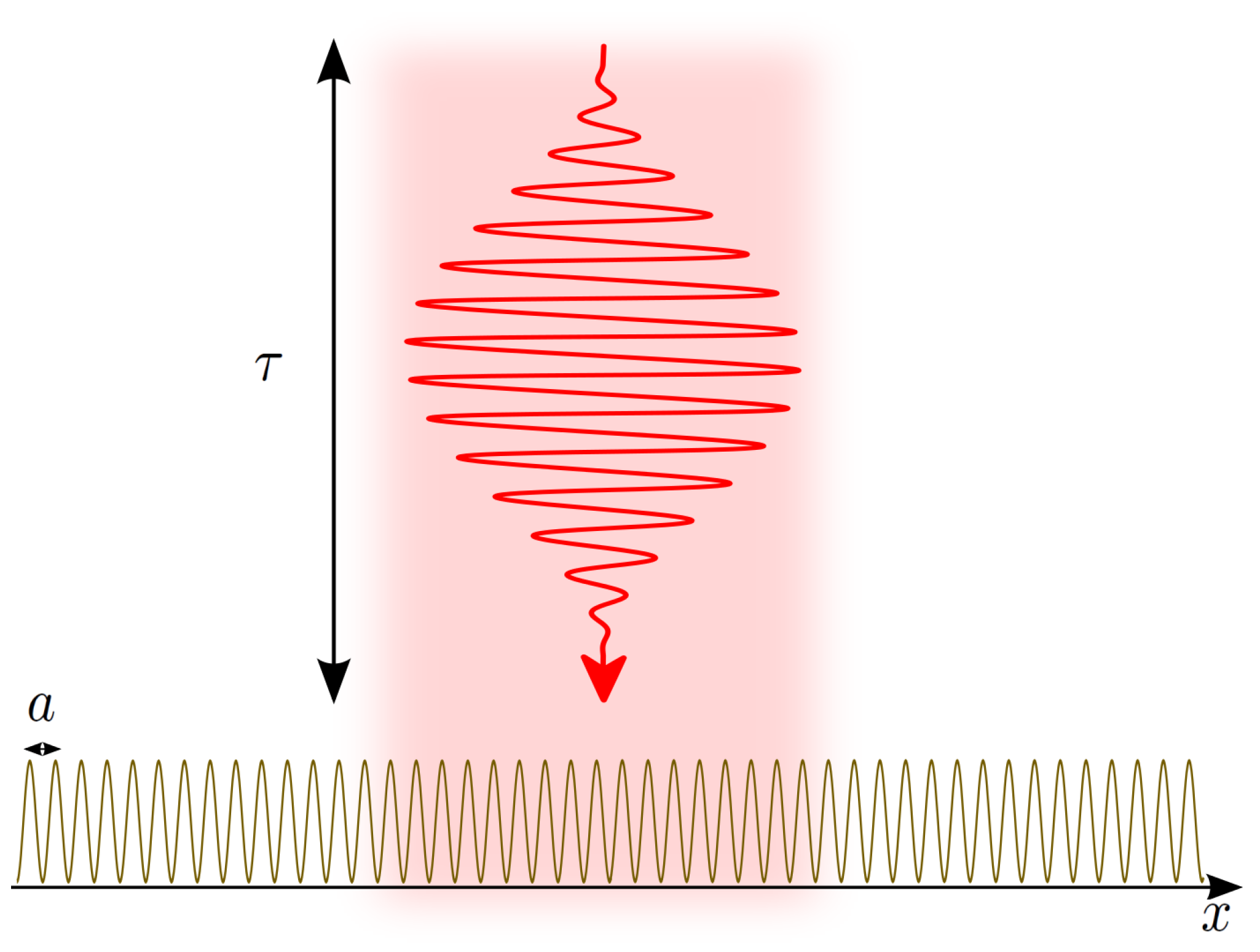
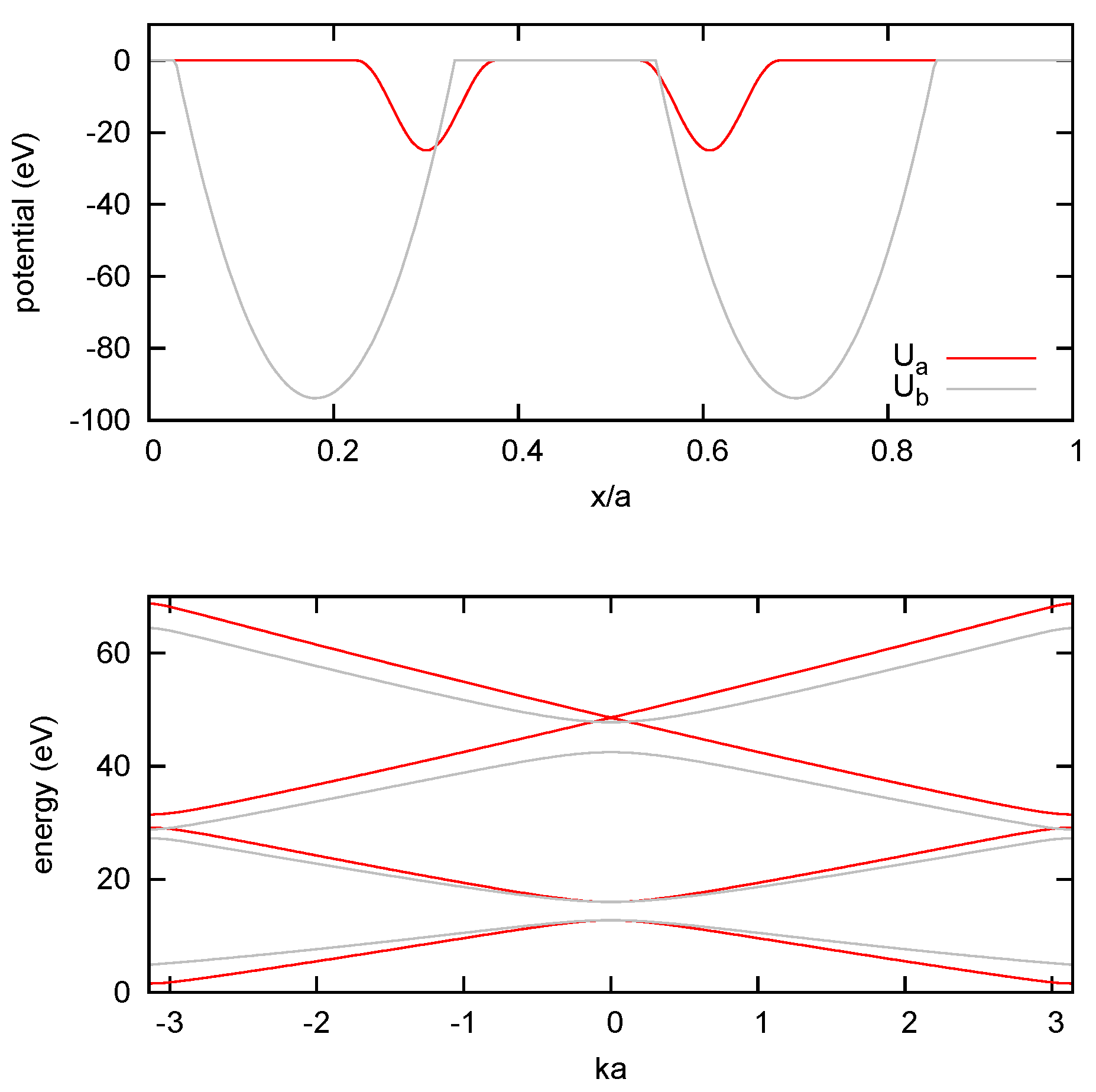
In order to simplify the calculations, we are going to use a one-dimensional model in the following (see Figure 1). Note that this can be adequate for linearly polarized excitations. We consider two model potentials that have one point in common: both produce a band scheme with a (maximal) gap of $3.2eV$, which corresponds to the case of the ZnO crystal. The explicit form of the first potential is the following:

$$U^{\left(a\right)}\left(x\right)=-U_0^{\left(a\right)}\sum _{i=1}^2{cos}^2\left[\pi \left(x-x_i^{\left(a\right)}\right)/{\Delta }^a\right],$$

(6)

where the functions ${cos}^2$ are assumed to be zero when their arguments are not in the interval $[-\pi /2,\pi /2]$. The parameters are: $U_0^{\left(a\right)}=25eV$, ${\Delta }^{\left(a\right)}/a=0.15$, $x_1^{\left(a\right)}/a=0.3$ and $x_2^{\left(a\right)}/a=0.607$, where a denotes the lattice constant. $U^{\left(b\right)}$ is also a double-well potential, as given by:

$$U^{\left(b\right)}\left(x\right)=\mathcal{N}\left[-U_{shift}^{\left(b\right)}+U_0^{\left(b\right)}{sinh}^2\left(\frac{x-x_1^{\left(b\right)}}{a}\right)\right]+\mathcal{N}\left[-U_{shift}^{\left(b\right)}+U_0^{\left(b\right)}{sinh}^2\left(\frac{x-x_2^{\left(b\right)}}{a}\right)\right],$$

(7)

where $\mathcal{N}\left(x\right)$ denotes the negative part of $x$, that is, $\mathcal{N}\left(x\right)=x$ when $x\le 0$, and zero otherwise. Additionally, $U_{shift}^{\left(b\right)}=93.861eV$, $U_0^{\left(b\right)}=4080.925eV$, $x_1^{\left(b\right)}/a=0.18$, and $x_2^{\left(b\right)}/a=0.7$. The potentials, together with the band structure that they induced, are shown in Figure 2. Note that, apart from the bandgap, these potentials correspond to considerably different band schemes; thus, they can be used to check to what extent our results depend on the particular choice of the model.

Inserting these potentials in the 1D version of Equation (2), we obtain the Bloch states ${\mathsf{\Psi }}_{n,k}\left(x\right)$. We use a finite number of k values, which are uniformly distributed in the first Brillouin zone $\left[-\pi /a,\pi /a\right]$, where a is the lattice constant. As a next step, we calculate the matrix elements $\langle n,k\left|H_0\right|n^{\prime },k^{\prime }\rangle$ and $\langle n,k\left|p_x\right|n^{\prime },k^{\prime }\rangle$, which are both proportional to ${\delta }_{k{k}^{\prime }}$. Using these matrix elements and the initial conditions (3), the dynamical equation (4) can be integrated by numerical means. In these calculations, we assume that the only nonzero component of the vector potential is given by:

$$A_x(x,t)=\left\{\begin{array}{c}{A}_0{sin}^2(\pi t/\tau )sin({\omega }_{L}t+\phi ),\mathrm{if}t\in [0,\tau ],\hfill \\ 0\mathrm{otherwise},\hfill \end{array}\right.,$$

(8)

where $\tau$ measures the duration of the pulse, and ${\omega }_L=2\pi c/\left(3\mathsf{\mu }\mathrm{m}\right)$ denotes the central frequency of the excitation. In dipole approximation, the vector potential has no spatial dependence. Note that since we are considering relatively long pulses (≈30 optical cycles at intensity FWHM), the results are expected to be almost independent of the carrier-envelope phase, $\phi$. Therefore, we use $\phi =0$ in the rest of the paper.

When the time-dependent density matrix is obtained, the expectation value of the kinetic momentum can be calculated in a way that leads to the function $J\left(t\right)$ (the 1D version of Equation (5)), and the fast Fourier transform provides the HHG spectra.

The fact that all transitions are vertical in velocity gauge allows us to calculate the contribution of every value of k to the net current density separately. Not only is the time evolution of the projectors $|n_0,k\rangle \langle n_0,k|$ independent for different values of $k$, but as the initial conditions (3) show, there is no quantum mechanical interference between these states either. However, their contribution to J has to be added linearly, so these contributions do interfere. Technically, this means that we first have to construct $J\left(t\right)$ and then calculate its power spectrum (so it is not the power spectra corresponding to different values of k that have to be added). In the next section, we investigate how these interference phenomena determine the properties of the HHG spectra.

3. Results

3.1. General Properties of the HHG Spectra

The HHG spectra that can be obtained as described above, show a weak dependence on the number of the conduction bands that we take into account. According to our experience, for moderate exciting field intensities, a four-band model (VB + 3CBs) is sufficient in the sense that in adding more CBs, the results practically do not change. (Note that a peak field strength of $F_0=1$ GV/m, together with a focal spot size of around 50 microns and additional pulse parameters given in the caption of Figure 3, means pulse energies of the order of 0.01 mJ). Additionally, in order to see the physical meaning of the relevant parameter ranges, it is worth providing the ratio of some important energies and frequencies. For a peak field strength of 1 GV/m (that corresponds to 1.33 × 10¹¹ W/cm² peak intensity) and a characteristic lattice constant of 5 Å, the Bloch frequency ${\omega }_B=ae{F}_0/\hslash$ has the same order of magnitude as ${\omega }_L$ at ${\lambda }_L=3$ microns. $\hslash {\omega }_L$ is 7.7 times smaller than the minimal bandgap (3.2 eV), and more than 50 times smaller than the maximal bandgap (for both potentials). Considering $ae{F}_0$ to be the characteristic laser-induced energy, we find that it has the order of magnitude of a few eV, which is considerably below the binding energy of both of the potentials—see Figure 2.

As expected, the choice of the periodic potential U (as given by Equations (6) and (7)) also influences the resulting spectra. However, we found that the qualitative features of the HHG spectra to be discussed below, are general—that is, the same for both potentials. Therefore, apart from a single example (see the next subsection), we are not going to compare all the results for $U^{\left(a\right)}$ and $U^{\left(b\right)}$.

Figure 3 shows representative HHG spectra calculated using $U^{\left(a\right)}$. As can be seen, the usual structure of the high-order harmonic spectra can be identified in this Figure—the most dominant peak corresponds to the exciting frequency, and there is a plateau region with peaks of approximately the same heights, as well as a cutoff where the peaks disappear. A difference of several orders of magnitude can be observed between the maxima and minima of the spectra. Additionally, in this intensity regime, the cutoff scales linearly with the amplitude of the exciting field, in a qualitative agreement with experimental findings [17]. Quantitatively, however, we observe more harmonics than the ones seen in the experiment. For a more realistic model that takes e.g. propagation effects also into account, we can expect a better agreement. Furthermore, the increase of individual HH peaks as a function of the intensity of the excitation shows qualitative agreement with the experimental results—see Figure 4. Similarly to [17], the heights of the peaks follow a power law for low intensities, and we can also see a deviation from this law at higher intensities. Quantitatively, this change in behavior occurs slightly earlier than in the experimental data.

To summarize, our model can reproduce most of the qualitative features of the experimental spectra, but since neither the propagation, nor the decay effects beyond the phenomenological ones were taken into account, no strong quantitative agreement can be found. More specifically:

• The structure of the spectra (plateau, cutoff) can be reproduced;
• The cutoff depends linearly on the peak field strength of the excitation ($F_0$);
• The $F_0$-dependence of the heights of the HH peaks is characteristically the same as in the experiments.

On the other hand, there is no quantitative agreement, since:

• The cutoff appears for higher harmonics than in the experiment;
• The power law dependence of the HH peak heights on the exciting field strength breaks down earlier than in the experiment [17].

Additionally, since the high-frequency regime of the spectrum is noisier than its first part, we cannot reliably determine whether we can observe the appearance of a second plateau as in [23]. The appearance of even-order harmonics will be discussed in the next subsection.

Based on the properties collected above, we can conclude that our 1D model can reproduce most of the characteristic properties of the HHG spectra. Now, we investigate the physical reasons for the appearance of these properties.

3.2. Even and Odd Harmonics

As we have seen, it is possible to calculate spectra that result from any subset of k values chosen from the first Brillouin zone. In other words, we can artificially restrict the summation over k in Equation (3), and investigate how the interference of the contributions of these states as sources to the complete current density result in the net HHG signal.

Focusing on the practical absence of the even-order harmonics from the spectra, Figure 5 provides an explanation. As we can see, HHG signals corresponding to a given value of k contain all harmonics with approximately the same weights. However, as the example of Figure 5 shows, when we combine the current densities that result from the time evolution of a given k and its opposite, the even harmonics tend to disappear. That is, the fields emerging from the time evolution of states that—without the external field—have phase velocities with the same magnitudes but opposite signs, interfere constructively for the odd harmonics, and destructively for the even ones. Additionally, this result does not depend on the particular choice of the model potential U, since it is visible for both $U^{\left(a\right)}$ and $U^{\left(b\right)}$.

Now, it is important to emphasize that the question of whether even-order harmonics will appear or not, can be decided using very fundamental, symmetry based considerations. Besides inversion symmetry [51], the periodicity of the excitation is also crucial (we thank one of our referees for drawing our attention to this point), since destructive interferences appear in consecutive half-cycles. In this way, the inversion symmetry of the material, together with the repetition of the field with the opposite sign in the next half-cycle, is responsive for the suppression of even-order harmonics. However, when no real-space symmetry can be associated to the emitters (like in the case of abstract two-level systems [52]), generally both odd and even order harmonics appear. As we see here, when a system of few-level quantum systems can be related to a physical system in real space, this situation changes, but in this case, the interference of fields emitted by all individual few-level systems is needed.

The trivial method of discovering the role of inversion in our treatment would be comparing the spectra that correspond to potentials with and without inversion symmetry. However, using different pairs of potentials (not only $U^{\left(a\right)}$ and $U^{\left(b\right)}$), we observed no qualitative difference, and the even-order harmonics were practically always missing. This effect can originate from the dimensionality of the model, since working in one dimension means assuming that only a very narrow set of k vectors from the orthogonal plane plays a relevant role in the time evolution, and this may not be the case for real materials.

On the other hand, since the appearance of the even-order harmonics is not determined by the crystal structure alone, the symmetry of the exciting field is equally important. The ”half-cycle by half-cycle sign change symmetry” of a long, many-cycle infrared pulse can be broken by adding a slowly varying, few-cycle electromagnetic pulse, such as in the THz regime. The result of this kind of ”THz-assisted” HHG is shown by Figure 6. As we can see, in this case, the even-order harmonics appear—practically as strongly as the odd-order ones—already in a 1D model.

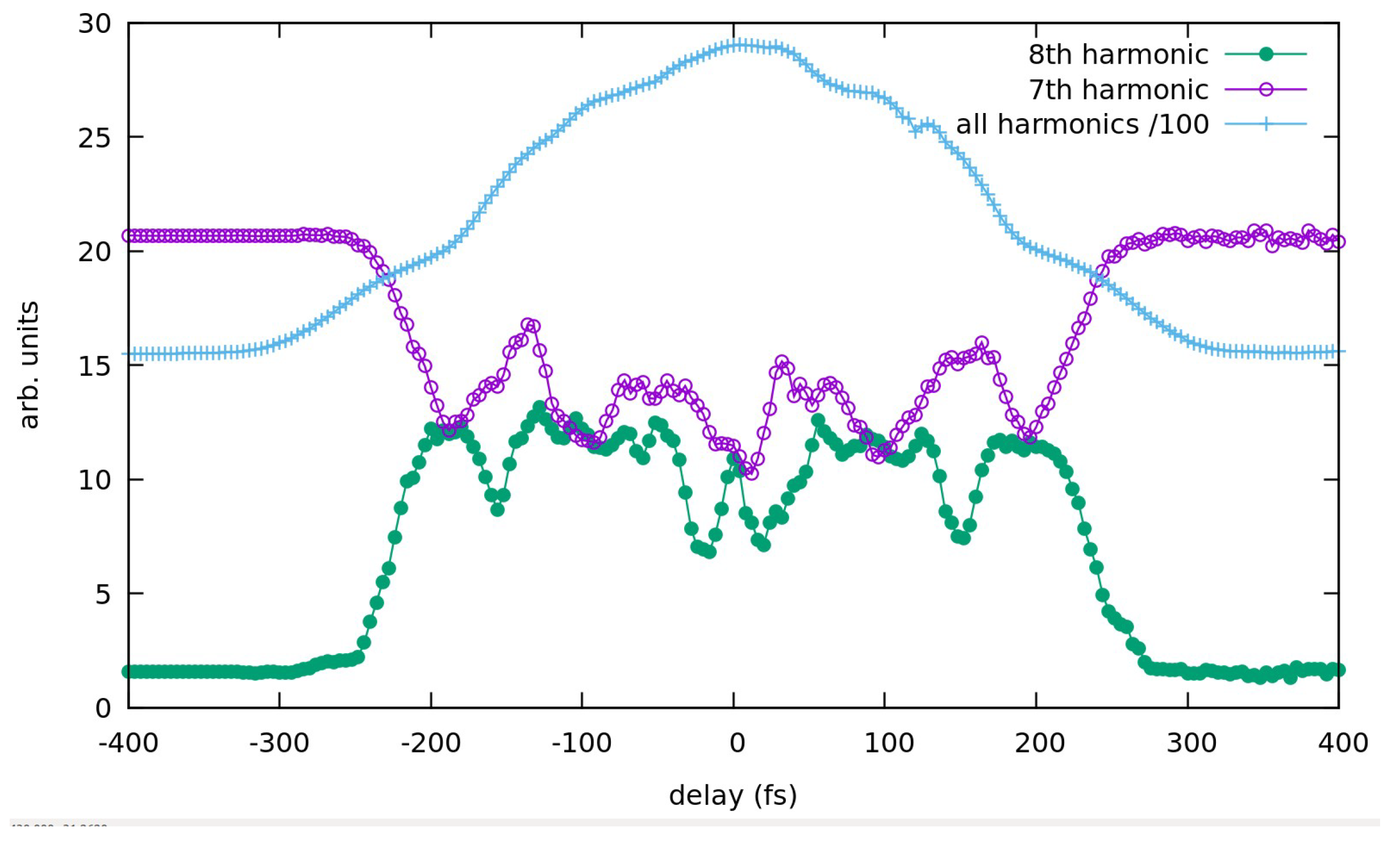
In order to see this in more detail, we investigated the role of the delay between the THz and the infrared pulses. (Note that this delay was zero for Figure 6.) As we can see in Figure 7, when there is no overlap between the pulses, the strength of the harmonics are practically the same as without the THz radiation, regardless of the sign of the delay. This underlines the fact that it is the infrared radiation that produces high harmonics, and the THz pulse itself is not intense enough in this sense. However, the overall HH gain increases when the pulses considerably overlap—it has a maximum at zero delay, that is, when the peak value of the net electric field is maximal.

For the individual harmonics, we can see that in accordance with the previous results, the presence of the THz radiation increases the height of the even-order harmonic peaks. (Note that in order to decrease numerical errors, Figure 7 shows the intergral of the spectrum around the given HH frequencies.) On the other hand, surprisingly, odd-order harmonics become weaker when the infrared and the THz pulses overlap considerably. For the strength of the seventh harmonic, as it is shown by Figure 7, the dependence on the delay exhibits strong modulations with the half-cycle period of the THz field. For the case of the eighth harmonic, this is less obvious, and fast modulations are more apparent.

Although the qualitative features of Figure 7 can be explained, and they are in agreement with Figure 6, it is clear that in order to completely explore the case of THz-assisted HHG with different delays, a more detailed investigation is needed—however, this is beyond the scope of the current paper.

It is also worth plotting the populations in the four bands that we took into account. The result is shown by Figure 8, where it can be seen why, in the intensity range we considered, four bands were enough for the appropriate description: the population of the third conduction band is practically negligible. As a closer look (and the Fourier transform as well) reveals, harmonic frequencies modulate the time evolution of the populations. Finally, it is worth mentioning that for multi-cycle infrared excitations (without the THz field), the populations in the conduction bands were practically zero when the pulse was over. On the other hand, with the additional THz field, these final populations increased orders of magnitude (definitely above the level of the numerical errors), but they still had the order of magnitude of 10⁻⁶–10⁻⁸.

3.3. The Position of the Cutoff

For M CBs and a given value of $k$, we have to calculate the dynamics of an $(M+1)$-level quantum system. For long excitations, Floquet’s method [53] can be applied, and (at least for $M=1$, see [54]) the cutoff of the HHG spectrum can be analytically estimated. However, in general, these cutoffs will be different for different values of k, since the parameters (the k-dependent bandgap and the matrix elements of the Hamiltonian) will also be different. Additionally, different values of k contribute to the net HHG signal to a different extent: the states close to the minimal bandgap ($k=0$ in our case) are the most dominant, but a very narrow set of states around $k=0$ cannot reproduce the complete spectrum. On the other hand, as expected, states close to the boundaries of the Brillouin zone ($ka=\pm \pi$, where the bandgap is the largest) modify the spectra negligibly.

As a demonstration, Figure 9 shows how the net HHG signal and the physically measurable cutoff is being built up as a superposition of the individual contributions from different values of k that cover intervals of increasing sizes around $k=0$. (The corresponding parts of the valence band are schematically shown by the insets.) Note that, as we saw in the previous subsection, the symmetry of these intervals around zero provides the dominance of the odd-order HHG peaks in the spectrum over the even-order ones. As we can see, although a narrow interval of k values around 0 can produce qualitatively correct HHG spectra, the combined effect of practically all states is needed for the spectra that can be detected.

4. Summary

In this paper, we considered a quantum mechanical model for the generation of high-order harmonics in bulk solids. The crystal was assumed to be initially in thermal equilibrium, with only the valence band being populated. We investigated the contribution of different initial states to the HH radiation, and showed that important aspects of the HHG spectra were strongly influenced by the interference of these contributions. According to our calculations, the absence of even-order harmonics can be viewed as a consequence of the destructive interference of currents that correspond to initial states with an opposite crystal momentum, $k$. This approach provides an intuitive picture behind the fundamental, symmetry-based argumentations. Interference effects were also shown to be related to the position of the cutoff.

References

- McPherson, A.; Gibson, G.; Jara, H.; Johann, U.; Luk, T.S.; McIntyre, I.A.; Boyer, K.; Rhodes, C.K. Studies of multiphoton production of vacuum-ultraviolet radiation in the rare gases. J. Opt. Soc. Am. B 1987, 4, 595–601. [Google Scholar] [CrossRef]
- Ferray, M.; L’Huillier, A.; Li, X.F.; Lompre, L.A.; Mainfray, G.; Manus, C. Multiple-harmonic conversion of 1064 nm radiation in rare gases. J. Phys. B At. Mol. Phys. 1988, 21, L31. [Google Scholar] [CrossRef]
- Farkas, G.; Tóth, C. Proposal for attosecond light pulse generation using laser induced multiple-harmonic conversion processes in rare gases. Phys. Lett. A 1992, 168, 447–450. [Google Scholar] [CrossRef]
- Hentschel, M.; Kienberger, R.; Spielmann, C.; Reider, G.A.; Milosevic, N.; Brabec, T.; Corkum, P.; Heinzmann, U.; Drescher, M.; Krausz, F. Attosecond metrology. Nature 2001, 414, 509. [Google Scholar] [CrossRef]
- Paul, P.M.; Toma, E.S.; Breger, P.; Mullot, G.; Augé, F.; Balcou, P.; Muller, H.G.; Agostini, P. Observation of a Train of Attosecond Pulses from High Harmonic Generation. Science 2001, 292, 1689–1692. [Google Scholar] [CrossRef] [PubMed]
- Drescher, M.; Hentschel, M.; Kienberger, R.; Tempea, G.; Spielmann, C.; Reider, G.A.; Corkum, P.B.; Krausz, F. X-ray Pulses Approaching the Attosecond Frontier. Science 2001, 291, 1923–1927. [Google Scholar] [CrossRef] [PubMed] [Green Version]
- Föhlisch, A.; Feulner, P.; Hennies, F.; Fink, A.; Menzel, D.; Sanchez-Portal, D.; Echenique, P.M.; Wurth, W. Direct observation of electron dynamics in the attosecond domain. Nature 2005, 436, 373–376. [Google Scholar] [CrossRef]
- Dudovich, N.; Smirnova, O.; Levesque, J.; Mairesse, Y.; Ivanov, M.Y.; Villeneuve, D.M.; Corkum, P.B. Measuring and controlling the birth of attosecond XUV pulses. Nat. Phys. 2006, 2, 781–786. [Google Scholar] [CrossRef]
- Scrinzi, A.; Yu Ivanov, M.; Kienberger, R.; Villeneuve, D.M. Attosecond physics. J. Phys. B At. Mol. Phys. 2006, 39, R1. [Google Scholar]
- Corkum, P.B.; Krausz, F. Attosecond science. Nat. Phys. 2007, 3, 381–387. [Google Scholar] [CrossRef]
- Eckle, P.; Pfeiffer, A.N.; Cirelli, C.; Staudte, A.; Dörner, R.; Muller, H.G.; Büttiker, M.; Keller, U. Attosecond Ionization and Tunneling Delay Time Measurements in Helium. Science 2008, 322, 1525–1529. [Google Scholar] [CrossRef]
- Krausz, F.; Stockman, M.I. Attosecond metrology: from electron capture to future signal processing. Nat. Photonics 2014, 8, 205–213. [Google Scholar] [CrossRef]
- Calegari, F.; Sansone, G.; Stagira, S.; Vozzi, C.; Nisoli, M. Advances in attosecond science. J. Phys. B At. Mol. Phys. 2016, 49, 062001. [Google Scholar] [CrossRef] [Green Version]
- Marangos, J.P. High-harmonic generation: Solid progress. Nat. Phys. 2011, 7, 97–98. [Google Scholar] [CrossRef]
- Quéré, F.; Thaury, C.; Monot, P.; Dobosz, S.; Martin, P.; Geindre, J.P.; Audebert, P. Coherent Wake Emission of High-Order Harmonics from Overdense Plasmas. Phys. Rev. Lett. 2006, 96, 125004. [Google Scholar] [CrossRef] [Green Version]
- Vincenti, H.; Monchocé, S.; Kahaly, S.; Bonnaud, G.; Martin, P.; Quéré, F. Optical properties of relativistic plasma mirrors. Nat. Commun. 2014, 5, 3403. [Google Scholar] [CrossRef]
- Ghimire, S.; DiChiara, A.D.; Sistrunk, E.; Agostini, P.; DiMauro, L.F.; Reis, D.A. Observation of high-order harmonic generation in a bulk crystal. Nat. Phys. 2011, 7, 138–141. [Google Scholar] [CrossRef]
- Ghimire, S.; DiChiara, A.D.; Sistrunk, E.; Szafruga, U.B.; Agostini, P.; DiMauro, L.F.; Reis, D.A. Redshift in the Optical Absorption of ZnO Single Crystals in the Presence of an Intense Midinfrared Laser Field. Phys. Rev. Lett. 2011, 107, 167407. [Google Scholar] [CrossRef]
- Ghimire, S.; DiChiara, A.D.; Sistrunk, E.; Ndabashimiye, G.; Szafruga, U.B.; Mohammad, A.; Agostini, P.; DiMauro, L.F.; Reis, D.A. Generation and propagation of high-order harmonics in crystals. Phys. Rev. A 2012, 85, 043836. [Google Scholar] [CrossRef]
- Ghimire, S.; Ndabashimiye, G.; DiChiara, A.D.; Sistrunk, E.; Stockman, M.I.; Agostini, P.; DiMauro, L.F.; Reis, D.A. Strong-field and attosecond physics in solids. J. Phys. B 2014, 47, 204030. [Google Scholar] [CrossRef] [Green Version]
- Schubert, O.; Hohenleutner, M.; Langer, F.; Urbanek, B.; Lange, C.; Huttner, U.; Golde, D.; Meier, T.; Kira, M.; Koch, S.W.; et al. Sub-cycle control of terahertz high-harmonic generation by dynamical Bloch oscillations. Nat. Photonic 2014, 8, 119–123. [Google Scholar] [CrossRef] [Green Version]
- Hohenleutner, M.; Langer, F.; Schubert, O.; Knorr, M.; Huttner, U.; Koch, S.W.; Kira, M.; Huber, R. Real-time observation of interfering crystal electrons in high-harmonic generation. Nature 2015, 523, 572–575. [Google Scholar] [CrossRef] [PubMed] [Green Version]
- Ndabashimiye, G.; Ghimire, S.; Wu, M.; Browne, D.A.; Schafer, K.J.; Gaarde, M.B.; Reis, D.A. Solid-state harmonics beyond the atomic limit. Nature 2016, 534, 520–523. [Google Scholar] [CrossRef]
- Goulielmakis, E.; Loh, Z.H.; Wirth, A.; Santra, R.; Rohringer, N.; Yakovlev, V.S.; Zherebtsov, S.; Pfeifer, T.; Azzeer, A.M.; Kling, M.F.; Leone, S.R.; Krausz, F. Real-time observation of valence electron motion. Nature 2010, 466, 739–743. [Google Scholar] [CrossRef]
- Schultze, M.; Ramasesha, K.; Pemmaraju, C.D.; Sato, S.A.; Whitmore, D.; Gandman, A.; Prell, J.S.; Borja, L.J.; Prendergast, D.; Yabana, K.; Neumark, D.M.; Leone, S.R. Attosecond band-gap dynamics in silicon. Science 2014, 346, 1348–1352. [Google Scholar] [CrossRef] [PubMed]
- You, Y.S.; Reis, D.A.; Ghimire, S. Anisotropic high-harmonic generation in bulk crystals. Nat. Phys. 2017, 13, 345–349. [Google Scholar] [CrossRef]
- Garg, M.; Zhan, M.; Luu, T.T.; Lakhotia, H.; Klostermann, T.; Guggenmos, A.; Goulielmakis, E. Multi-petahertz electronic metrology. Nature 2016, 538, 359–363. [Google Scholar] [CrossRef]
- Liu, H.; Li, Y.; You, Y.S.; Ghimire, S.; Heinz, T.F.; Reis, D.A. High-harmonic generation from an atomically thin semiconductor. Nat. Phys. 2017, 13, 262–265. [Google Scholar] [CrossRef]
- Han, S.; Kim, H.; Kim, Y.W.; Kim, Y.J.; Kim, S.; Park, I.Y.; Kim, S.W. High-harmonic generation by field enhanced femtosecond pulses in metal-sapphire nanostructure. Nat. Commun. 2016, 7, 13105. [Google Scholar] [CrossRef] [Green Version]
- Ghimire, S.; Reis, D. High-harmonic generation from solids. Nat. Phys. 2019, 15, 10. [Google Scholar] [CrossRef]
- Corkum, P.B. Plasma perspective on strong field multiphoton ionization. Phys. Rev. Lett. 1993, 71, 1994–1997. [Google Scholar] [CrossRef] [PubMed] [Green Version]
- Lewenstein, M.; Balcou, P.; Ivanov, M.Y.; L’Huillier, A.; Corkum, P.B. Theory of high-harmonic generation by low-frequency laser fields. Phys. Rev. A 1994, 49, 2117–2132. [Google Scholar] [CrossRef] [PubMed]
- Durach, M.; Rusina, A.; Kling, M.F.; Stockman, M.I. Predicted Ultrafast Dynamic Metallization of Dielectric Nanofilms by Strong Single-Cycle Optical Fields. Phys. Rev. Lett. 2011, 107, 086602. [Google Scholar] [CrossRef] [PubMed]
- Higuchi, T.; Stockman, M.I.; Hommelhoff, P. Strong-Field Perspective on High-Harmonic Radiation from Bulk Solids. Phys. Rev. Lett. 2014, 113, 213901. [Google Scholar] [CrossRef]
- Sansone, G.; Vozzi, C.; Stagira, S.; Nisoli, M. Nonadiabatic quantum path analysis of high-order harmonic generation: Role of the carrier-envelope phase on short and long paths. Phys. Rev. A 2004, 70, 013411. [Google Scholar] [CrossRef]
- Vampa, G.; McDonald, C.R.; Orlando, G.; Klug, D.D.; Corkum, P.B.; Brabec, T. Theoretical Analysis of High-Harmonic Generation in Solids. Phys. Rev. Lett. 2014, 113, 073901. [Google Scholar] [CrossRef]
- Vampa, G.; McDonald, C.; Fraser, A.; Brabec, T. High-Harmonic Generation in Solids: Bridging the Gap between Attosecond Science and Condensed Matter Physics. IEEE J. Sel. Top. Quantum Electron. 2015, 21, 1–10. [Google Scholar] [CrossRef]
- Lindberg, M.; Koch, S. Effective Bloch equations for semiconductors. Phys. Rev. B 1988, 38, 3342. [Google Scholar] [CrossRef]
- Kruchinin, S.; Korbman, M.; Yakovlev, V. Theory of strong-field injection and control of photocurrent in dielectrics and wide band gap semiconductors. Phys. Rev. B 2013, 87, 115201. [Google Scholar] [CrossRef]
- Lackner, F.; Březinová, I.; Sato, T.; Ishikawa, K.L.; Burgdörfer, J. High-harmonic spectra from time-dependent two-particle reduced-density-matrix theory. Phys. Rev. A 2017, 95, 033414. [Google Scholar] [CrossRef]
- Tancogne-Dejean, N.; Mücke, O.D.; Kärtner, F.X.; Rubio, A. Ellipticity dependence of high-harmonic generation in solids originating from coupled intraband and interband dynamics. Nat. Commun. 2017, 8, 745. [Google Scholar] [CrossRef]
- Tancogne-Dejean, N.; Mücke, O.D.; Kärtner, F.X.; Rubio, A. Impact of the Electronic Band Structure in High-Harmonic Generation Spectra of Solids. Phys. Rev. Lett. 2017, 118, 087403. [Google Scholar] [CrossRef] [PubMed]
- Földi, P. Gauge invariance and interpretation of interband and intraband processes in high-order harmonic generation from bulk solids. Phys. Rev. B 2017, 96, 035112. [Google Scholar] [CrossRef]
- Hawkins, P.; Ivanov, M.Y.; Yakovlev, V. Effect of multiple conduction bands on high-harmonic emission from dielectrics. Phys. Rev. A 2015, 87, 115201. [Google Scholar] [CrossRef]
- Takahashi, E.; Tosa, V.; Nabekawa, Y.; Midorikawa, K. Experimental and theoretical analyses of a correlation between pump-pulse propagation and harmonic yield in a long-interaction medium. Phys. Rev. A 2003, 68, 023808. [Google Scholar] [CrossRef]
- Kovács, K.; Balogh, E.; Hebling, J.; Toşa, V.; Varjú, K. Quasi-Phase-Matching High-Harmonic Radiation Using Chirped THz Pulses. Phys. Rev. Lett. 2012, 108, 193903. [Google Scholar] [CrossRef]
- Becker, P.C.; Fragnito, H.L.; Cruz, C.H.B.; Fork, R.L.; Cunningham, J.E.; Henry, J.E.; Shank, C.V. Femtosecond Photon Echoes from Band-to-Band Transitions in GaAs. Phys. Rev. Lett. 1988, 61, 1647–1649. [Google Scholar] [CrossRef]
- Hughes, R.C. Charge-Carrier Transport Phenomena in Amorphous SiO2: Direct Measurement of the Drift Mobility and Lifetime. Phys. Rev. Lett. 1973, 30, 1333–1336. [Google Scholar] [CrossRef]
- Vampa, G.; McDonald, C.R.; Orlando, G.; Corkum, P.B.; Brabec, T. Semiclassical analysis of high harmonic generation in bulk crystals. Phys. Rev. B 2015, 91, 064302. [Google Scholar] [CrossRef] [Green Version]
- Földi, P.; Benedict, M.G.; Yakovlev, V.S. The effect of dynamical Bloch oscillations on optical-field-induced current in a wide-gap dielectric. New J. Phys. 2013, 15, 063019. [Google Scholar] [CrossRef] [Green Version]
- Jiang, S.; Wei, H.; Chen, J.; Yu, C.; Lu, R.; Lin, C.D. Effect of transition dipole phase on high-order-harmonic generation in solid materials. Phys. Rev. A 2017, 96, 053850. [Google Scholar] [CrossRef]
- Gombkötő, A.; Czirják, A.; Varró, S.; Földi, P. Quantum-optical model for the dynamics of high-order-harmonic generation. Phys. Rev. A 2016, 94, 013853. [Google Scholar] [CrossRef]
- Floquet, G. Sur les équations différentielles linéaires a coefficients périodiques. Ann. École Norm. Sup. 1883, 12, 46–88. [Google Scholar] [CrossRef]
- Gauthey, F.I.; Garraway, B.M.; Knight, P.L. High harmonic generation and periodic level crossings. Phys. Rev. A 1997, 56, 3093–3096. [Google Scholar] [CrossRef] [Green Version]
Figure 1.
Schematic view of an external laser-driven periodic structure. The duration of the pulse is denoted by and the lattice constant of the 1D crystal is given by a. Note that, usually, the central wavelength of the incoming laser pulse is larger than , meaning that dipole approximation can be used.
Figure 2.
Top panel: The model potentials (red curve) and (grey curve) as a function of the coordinate x in a unit cell. The corresponding band schemes are shown in the bottom panel (where an additive scaling factor has been used in order to see more clearly that the band gaps are the same).
Figure 3.
Representative high-order harmonic spectra for different peak field strengths, which correspond to 0.083, 0.33, 0.75, and 1.33 × 10¹¹ W/cm2 peak intensities. The band scheme of the target is derived using the potential . Parameters: and . The frequency on the horizontal axis is given in units of .
Figure 4.
The height of the seventh and 11th high harmonic peak as a function of the peak field strength of the external field. (Please note the log–log scale.)
Figure 5.
The suppression of even-order harmonics. Panel (a) [(b)] corresponds to . In both panels, the contributions of given values of k is shown together with that of and their combined effect, for parameters (2.13 × 10¹² W/cm2 peak intensity), and .
Figure 6.
The appearance of even-order harmonics. Panel (a) infrared excitation, panel (b) THz assisted infrared excitation. The time dependences of the vector potentials of the exciting fields are shown by the insets, where the units for the horizontal and vertical axes are fs and GV·fs/m, respectively. Panel (c) shows the current density J, which is the source of the HH radiation.
Figure 7.
The contribution of different frequency ranges to the HHG radiation as a function of the delay between the infrared and the THz pulses for the same amplitudes as in Figure 6. Negative delays mean that the THz pulse arrives first. For the nth individual harmonic, the integral of the spectrum for an interval of the length of that is centered around is shown. For ”all harmonics”, the integration runs from to .
Figure 8.
The normalized populations in the bands we considered as a function of time. The left subfigure corresponds to purely infrared excitation, while there is an additional long wavelength, THz field for the right subfigure. The corresponding waveforms can be seen in the insets of Figure 6.
Figure 9.
Contributions of different parts of the valence band (represented by red color above the dotted vertical lines in the insets) to the HHG spectra as calculated using the potential . Parameters: (0.33 × 10¹¹ W/cm2 peak intensity) and . Note that the physical, measurable spectrum is the topmost one, where all initial states from the VB of the first Brillouin zone contribute to the radiation.
© 2019 by the authors. Licensee MDPI, Basel, Switzerland. This article is an open access article distributed under the terms and conditions of the Creative Commons Attribution (CC BY) license (http://creativecommons.org/licenses/by/4.0/).
Share and Cite
MDPI and ACS Style
Szaszkó-Bogár, V.; Földi, P.; Magashegyi, I.; Varjú, K. Interference-Induced Phenomena in High-Order Harmonic Generation from Bulk Solids. Appl. Sci. 2019, 9, 1572. https://doi.org/10.3390/app9081572
AMA Style
Szaszkó-Bogár V, Földi P, Magashegyi I, Varjú K. Interference-Induced Phenomena in High-Order Harmonic Generation from Bulk Solids. Applied Sciences. 2019; 9(8):1572. https://doi.org/10.3390/app9081572
Chicago/Turabian StyleSzaszkó-Bogár, Viktor, Péter Földi, István Magashegyi, and Katalin Varjú. 2019. "Interference-Induced Phenomena in High-Order Harmonic Generation from Bulk Solids" Applied Sciences 9, no. 8: 1572. https://doi.org/10.3390/app9081572
Note that from the first issue of 2016, this journal uses article numbers instead of page numbers. See further details here.