Analytical Theory of Attosecond Transient Absorption Spectroscopy of Perturbatively Dressed Systems

Abstract

A theoretical description of attosecond transient absorption spectroscopy for temporally and spatially overlapping XUV and optical pulses is developed, explaining the signals one can obtain in such an experiment. To this end, we employ a two-stage approach based on perturbation theory, which allows us to give an analytical expression for the transient absorption signal. We focus on the situation in which the attosecond XUV pulse is used to create a coherent superposition of electronic states. As we explain, the resulting dynamics can be detected in the spectrum of the transmitted XUV pulse by manipulating the electronic wave packet using a carrier-envelope-phase-stabilized optical dressing pulse. In addition to coherent electron dynamics triggered by the attosecond pulse, the transmitted XUV spectrum encodes information on electronic states made accessible by the optical dressing pulse. We illustrate these concepts through calculations performed for a few-level model.

1. Introduction

Transient absorption spectroscopy is a well-known technique for studying quantum dynamics on the femtosecond time scale [1,2]. When applying an external electromagnetic field, it is possible to modify the absorption cross-section of an XUV or X-ray probe pulse. This allows observing the dynamics driven in the system by the field. Time-resolved spectroscopy is applied today to all states of matter, including the gas, liquid, solid, and plasma phases, as well as large biomolecules [3,4,5,6,7,8,9,10,11,12,13,14,15].

As a function of the intensity of the applied external electromagnetic field different processes can be studied. In the case of optical tunnel ionization, probing after the strong-field pump pulse provides spectroscopic information about the residual ion, such as ion quantum state distributions [16,17] and orbital alignment [18,19]. At lower field strengths, laser-dressing and molecular alignment effects may be investigated [20,21,22,23,24,25,26,27,28].

In the past, measurements were typically performed in the infrared, visible, and ultraviolet spectral regions, using femtosecond or longer laser pulses [29,30]. Transient absorption spectroscopy was also performed with soft and hard X-rays down to time scales of picoseconds [31,32]. About ten years ago, soft X-ray transient absorption was demonstrated for femtosecond resolved probing in the gas phase [17] and condensed phase [33] by using high-order harmonics.

The advent of attosecond light pulses [34,35,36,37,38] has opened up the possibility of studying fundamental questions related to the quantum dynamics of electrons on their natural time scale. Particularly, attosecond transient absorption (ATA) spectroscopy [39] gives access to ultrafast dynamics of bound and autoionizing electronic states in rare gas atoms, molecules, and solids. If the attosecond pulse is used to initiate the electronic dynamics, it coherently populates bright (dipole allowed) states, forming a wave packet. The coherence between the initial (ground) state and each excited state gives rise to a nonstationary polarization. The presence of another electromagnetic field—a dressing field—affects the absorption of the attosecond pulse and, thus, provides control of the electronic wave packet created. Various dynamical aspects of the launched wave packet are imprinted in the delay-dependent absorption spectra.

A theoretical analysis of the ATA signal is crucial for understanding and maximizing its information content [40,41,42,43,44,45,46,47,48,49,50]. The goal of the current work is to provide an elementary explanation of the signals one can obtain in ATA experiments. We perform a perturbative analysis of the transient absorption signal as a function of the time delay between the attosecond excitation pulse and the femtosecond dressing pulse. Furthermore, through numerical calculations for a model atom, we illustrate how the ATA signal reveals the real-time attosecond dynamics of the system.

2. Formal Analysis

For the theoretical description of the processes of relevance here the semiclassical approximation may be used, by treating the electronic system under study as a quantum object and using the classical Maxwell equations for the electromagnetic field. The electromagnetic field can be described using perturbation theory in the weak-field case, where the Keldysh parameter $\gamma =\sqrt{\frac{I_p}{2U_p}}$ [51] is $\gamma \gg 1$ ($I_p$ is the ionization potential and $U_p$ is the pondermotive potential), or must be treated nonperturbatively in the strong-field case $\gamma <1$. In view of the rather small pulse energies of currently available attosecond sources, perturbation theory may be considered an excellent framework for treating the effect of the attosecond pulse. The dressing pulse is often not too strong and so that perturbation theory can be used as well.

In the current work we build on the theoretical description of ATA spectroscopy developed in Ref. [41] and extend it by performing a perturbative analysis of the impact of the dressing field. In contrast to Ref. [41], where the optical field was assumed to be so strong that it causes tunnel ionization even in the electronic ground state, we here consider the situation where the optical dressing field only affects the electronic states that are reached after absorbing an XUV photon from the attosecond pulse.

2.1. XUV One-Photon Absorption Cross-Section

We make the electric dipole approximation and assume that the attosecond pulse and the dressing pulse are both linearly polarized along the z-axis. Following the logic presented in Ref. [41], we start by solving the time-dependent Schrödinger equation:

$$i\frac{\partial }{\partial t}|\mathrm{\Psi },t\rangle =\widehat{H}\left(t\right)|\mathrm{\Psi },t\rangle ,$$

(1)

$$\widehat{H}\left(t\right)={\widehat{H}}_0-E_0-{\epsilon }_d\left(t\right)\widehat{Z}-{\epsilon }_x\left(t\right)\widehat{Z},$$

(2)

where $H_0$ is the unperturbed Hamiltonian of the electronic system, $E_0$ is the system ground-state energy, $\widehat{Z}$ is the z-component of the electric dipole operator, and ${\epsilon }_d\left(t\right)$ and ${\epsilon }_x\left(t\right)$ are the dressing and attosecond (XUV) electric fields, respectively. Assuming the effect of the attosecond pulse can be treated perturbatively, the solution of Equation (1) is:

$$|\mathrm{\Psi },t\rangle =|{\mathrm{\Psi }}_d{,t\rangle +|\mathrm{\Psi },t\rangle }^{\left(1\right)}+\dots ,$$

(3)

where $|{\mathrm{\Psi }}_d,t\rangle$ is the electronic state vector in the absence of the attosecond pulse and ${|\mathrm{\Psi },t\rangle }^{\left(1\right)}$ is the first-order correction with respect to the attosecond pulse. We employ the time-evolution operator ${\widehat{U}}_d(t,t_0)$ to determine the optically dressed state vector $|{\mathrm{\Psi }}_d,t\rangle$:

$$|{\mathrm{\Psi }}_d,t\rangle ={\widehat{U}}_d(t,t_0)|{\mathrm{\Psi }}_0,t_0\rangle .$$

(4)

Here $t_0$ is a time before the system is optically dressed and $|{\mathrm{\Psi }}_0,t_0\rangle =|{\mathrm{\Psi }}_0\rangle$ is the initial state. The dipole moment of the electronic system along the z-axis can be expressed as:

$$D\left(t\right)=\langle \mathrm{\Psi },t|\widehat{Z}|\mathrm{\Psi },t\rangle =D_{HG}\left(t\right)+D^{\left(1\right)}\left(t\right)+\dots$$

(5)

The term $D_{HG}\left(t\right)$ describes harmonic generation driven by the dressing pulse only, and $D^{\left(1\right)}\left(t\right)$ is the dipole moment correction to first order with respect to ${\epsilon }_x\left(t\right)$:

$$D_{HG}\left(t\right)=\langle {\mathrm{\Psi }}_d,t|\widehat{Z}|{\mathrm{\Psi }}_d,t\rangle ,$$

(6)

$$D^{\left(1\right)}\left(t\right)=i\underset{-\infty }{\overset{t}{\int }}d{t}^{\prime }{\epsilon }_x\left(t^{\prime }\right)\langle {\mathrm{\Psi }}_d,t|\widehat{Z}{\widehat{U}}_d(t,t^{\prime })\widehat{Z}|{\mathrm{\Psi }}_d,t^{\prime }\rangle +c.c.$$

(7)

In the following, we will separate the t dependence in $\langle {\mathrm{\Psi }}_d,t|\widehat{Z}{\widehat{U}}_d(t,t^{\prime })\widehat{Z}|{\mathrm{\Psi }}_d,t^{\prime }\rangle$ from the $t^{\prime }$ dependence. To this end, we employ the following identity:

$${\widehat{U}}_d(t,t^{\prime })={\widehat{U}}_d(t,t_0){\widehat{U}}_d^{-1}(t^{\prime },t_0),$$

(8)

which is correct for any reference time $t_0$. For reasons that will become clearer in Section 2.2, we write explicitly ${\widehat{U}}_d^{-1}(t^{\prime },t_0)$ rather than ${\widehat{U}}_d^{†}(t^{\prime },t_0)$.

Assuming that the attosecond pulse is shorter than all relevant electronic time scales [41], we approximate it by a delta function ${\epsilon }_x\left(t\right)=A_x\delta (t-\tau )$, where $\tau$ is the moment when the attosecond pulse interacts with the system. Hence, employing Equations (7) and (8), the dipole moment correction along the z-axis can be written as:

$$\begin{array}{cc}\hfill D^{\left(1\right)}\left(t\right)& =i\sum _f\left[\underset{-\infty }{\overset{t}{\int }}d{t}^{\prime }{\epsilon }_x\left(t^{\prime }\right)F_{0f}\left(t\right)F_{f0}\left(t^{\prime }\right)-\underset{-\infty }{\overset{t}{\int }}d{t}^{\prime }{\epsilon }_x\left(t^{\prime }\right)F_{0f}^{\ast }\left(t\right)F_{f0}^{\ast }\left(t^{\prime }\right)\right]\hfill \\ & =i{A}_x\sum _f\left[F_{0f}\left(t\right)F_{f0}\left(\tau \right)-F_{0f}^{\ast }\left(t\right)F_{f0}^{\ast }\left(\tau \right)\right]\theta (t-\tau ),\hfill \end{array}$$

(9)

where $\theta (t-\tau )$ is the Heaviside function. The functions $F_{mn}\left(t\right)$ in Equation (9) represent transition dipole matrix elements between optically dressed states $|{\mathrm{\Psi }}_m\rangle$ and $|{\mathrm{\Psi }}_n\rangle$:

$$\begin{array}{c}{F}_{mn}\left(t\right)=\langle {\mathrm{\Psi }}_m|{\widehat{U}}_d^{-1}(t,t_0)\widehat{Z}{\widehat{U}}_d(t,t_0)|{\mathrm{\Psi }}_n\rangle .\hfill \end{array}$$

(10)

The XUV one-photon cross-section of the system is given by [41]:

$${\sigma }^{\left(1\right)}\left(\omega \right)=\frac{4\pi \omega }{c}\mathrm{Im}\left[\frac{{\tilde{D}}^{\left(1\right)}\left(\omega \right)}{{\tilde{\epsilon }}_x\left(\omega \right)}\right],$$

(11)

where ${\tilde{D}}^{\left(1\right)}\left(\omega \right)$ is the Fourier transform of $D^{\left(1\right)}\left(t\right)$. Analogously, ${\tilde{\epsilon }}_x\left(\omega \right)$ is the Fourier transform of ${\epsilon }_x\left(t\right)$. Using Equation (9) and taking into account that the dipole moment $D^{\left(1\right)}\left(t\right)$ is a real function, we obtain from Equation (11):

$$\begin{array}{cc}\hfill {\sigma }^{\left(1\right)}(\omega ,\tau )& =i\frac{4\pi \omega }{c}\sum _f\underset{-\infty }{\overset{\infty }{\int }}dt\left[F_{0f}\left(t\right)F_{f0}\left(\tau \right)-F_{0f}^{\ast }\left(t\right)F_{f0}^{\ast }\left(\tau \right)\right]\theta (t-\tau )\mathrm{Im}\left[e^{i\omega (t-\tau )}\right]\hfill \\ & =\frac{2\pi \omega }{c}\sum _f\underset{\tau }{\overset{\infty }{\int }}dt\left[F_{0f}\left(t\right)e^{i\omega t}{F}_{f0}\left(\tau \right)e^{-i\omega \tau }-F_{0f}\left(t\right)e^{-i\omega t}{F}_{f0}\left(\tau \right)e^{i\omega \tau }+c.c.\right].\hfill \end{array}$$

(12)

In the following subsection we perform a perturbative analysis of the impact of the dressing field, to understand the spectroscopic properties of the functions $F_{mn}\left(t\right)$ and, thus, of ${\sigma }^{\left(1\right)}(\omega ,\tau )$.

2.2. Perturbative Treatment of the Dressing Pulse

Using perturbation theory, the time-evolution operator ${\widehat{U}}_d(t,t_0)$ in the presence of the dressing field [see Equation (4)] can be written as follows:

$$\begin{array}{cc}\hfill {\widehat{U}}_d(t,t_0)& =e^{-i({\widehat{H}}_0-E_0)(t-t_0)}\left[1-i{\int }_{t_0}^{t}d{t}^{\prime }{\widehat{V}}_d\left(t^{\prime }\right){\widehat{U}}_d^I(t^{\prime },t_0)\right]\hfill \\ & =e^{-i({\widehat{H}}_0-E_0)(t-t_0)}\left[1-i{\int }_{t_0}^{t}d{t}^{\prime }{\widehat{V}}_d\left(t^{\prime }\right)-{\int }_{t_0}^{t}d{t}^{\prime }{\int }_{t_0}^{t^{\prime }}d{t}^{″}{\widehat{V}}_d\left(t^{\prime }\right){\widehat{V}}_d\left(t^{″}\right)+\dots \right],\hfill \end{array}$$

(13)

where

$${\widehat{U}}_d^I(t,t_0)=1-i\underset{t_0}{\overset{t}{\int }}d{t}^{\prime }{\widehat{V}}_d\left(t^{\prime }\right){\widehat{U}}_d^I(t^{\prime },t_0)$$

(14)

is the time-evolution operator in the interaction picture and

$${\widehat{V}}_d\left(t\right)=-{\epsilon }_d\left(t\right)e^{i\{{\widehat{H}}_0-E_0\}(t-t_0)}\widehat{Z}{e}^{-i\{{\widehat{H}}_0-E_0\}(t-t_0)}$$

(15)

is the perturbation by the optical dressing field.

When evaluating Equation (9), we make use of a complete set of eigenstates of ${\widehat{H}}_0$. Because the excited states accessed may lie in the electronic continuum, this involves, strictly speaking, an integration over states. However, by focusing on bound states and autoionizing states only, we replace the integration by a summation over a discrete set of states $|{\mathrm{\Psi }}_f\rangle$ with a complex energy:

$${\widehat{H}}_0|{\mathrm{\Psi }}_f\rangle =(E_f-i\frac{{\mathrm{\Gamma }}_f}{2})|{\mathrm{\Psi }}_f\rangle .$$

(16)

Here $E_f$ is the real part of the energy and the non-negative real number ${\mathrm{\Gamma }}_f$ is the decay rate of the state $|{\mathrm{\Psi }}_f\rangle$ (${\mathrm{\Gamma }}_f=0$ for bound states). As a consequence of this choice, ${\widehat{H}}_0$ is not Hermitian, and, therefore, the time-evolution operator ${\widehat{U}}_d$ is not unitary, i.e., ${\widehat{U}}_d^{-1}(t,t_0)\ne {\widehat{U}}_d^{†}(t,t_0)$. This is important, because in the analytical treatment that follows, we will require the inverse of ${\widehat{U}}_d(t,t_0)$:

$$\begin{array}{cc}\hfill {\widehat{U}}_d^{-1}(t,t_0)& =\left[1+i{\int }_{t_0}^{t}d{t}^{\prime }{\left({\widehat{U}}_d^I(t^{\prime },t_0)\right)}^{-1}{\widehat{V}}_d\left(t^{\prime }\right)\right]e^{i({\widehat{H}}_0-E_0)(t-t_0)}\hfill \\ & =\left[1+i{\int }_{t_0}^{t}d{t}^{\prime }{\widehat{V}}_d\left(t^{\prime }\right)-{\int }_{t_0}^{t}d{t}^{\prime }{\int }_{t_0}^{t^{\prime }}d{t}^{″}{\widehat{V}}_d\left(t^{″}\right){\widehat{V}}_d\left(t^{\prime }\right)+\dots \right]e^{i({\widehat{H}}_0-E_0)(t-t_0)},\hfill \end{array}$$

(17)

which differs from ${\widehat{U}}_d^{†}(t,t_0)$ as conjugation is not applied to the Hamiltonian ${\widehat{H}}_0$.

We now apply Equations (13) and (17) to Equation (10). Resonant excitation involving XUV light tends to lead to the formation of an inner-shell hole accompanied by an excited electron (for atoms heavier than helium). For a given inner-shell hole, the decay rate is relatively insensitive to the state of the excited electron. Thus, we assume the decay rates to be equal to each other for all states (${\mathrm{\Gamma }}_n={\mathrm{\Gamma }}_f$), except for the ground state (${\mathrm{\Gamma }}_0=0$). Consequently, through second order in the dressing field, $F_{f0}$ can be decomposed as follows:

$$\begin{array}{cc}\hfill F_{f0}\left(t\right)=& F_{f0}^{00}\left(t\right)+F_{f0}^{01}\left(t\right)+F_{f0}^{10}\left(t\right)+F_{f0}^{02}\left(t\right)+F_{f0}^{20}\left(t\right)+F_{f0}^{11}\left(t\right)+\dots \hfill \\ \hfill =& f_{f0}^{00}\left(t\right)e^{\frac{{\mathrm{\Gamma }}_f}{2}t}\langle {\mathrm{\Psi }}_f|\widehat{Z}|{\mathrm{\Psi }}_0\rangle \hfill \\ & +\sum _a{f}_{fa0}^{01}\left(t\right)e^{\frac{{\mathrm{\Gamma }}_f}{2}t}\langle {\mathrm{\Psi }}_f|\widehat{Z}|{\mathrm{\Psi }}_a\rangle \langle {\mathrm{\Psi }}_a|\widehat{Z}|{\mathrm{\Psi }}_0\rangle \hfill \\ & +\sum _{\alpha }{f}_{f\alpha 0}^{10}\left(t\right)e^{\frac{{\mathrm{\Gamma }}_f}{2}t}\langle {\mathrm{\Psi }}_f|\widehat{Z}|{\mathrm{\Psi }}_{\alpha }\rangle \langle {\mathrm{\Psi }}_{\alpha }|\widehat{Z}|{\mathrm{\Psi }}_0\rangle \hfill \\ & +\sum _{ab}{f}_{fba0}^{02}\left(t\right)e^{\frac{{\mathrm{\Gamma }}_f}{2}t}\langle {\mathrm{\Psi }}_f|\widehat{Z}|{\mathrm{\Psi }}_b\rangle \langle {\mathrm{\Psi }}_b|\widehat{Z}|{\mathrm{\Psi }}_a\rangle \langle {\mathrm{\Psi }}_a|\widehat{Z}|{\mathrm{\Psi }}_0\rangle \hfill \\ & +\sum _{\alpha \beta }{f}_{f\alpha \beta 0}^{20}\left(t\right)e^{\frac{{\mathrm{\Gamma }}_f}{2}t}\langle {\mathrm{\Psi }}_f|\widehat{Z}|{\mathrm{\Psi }}_{\alpha }\rangle \langle {\mathrm{\Psi }}_{\alpha }|\widehat{Z}|{\mathrm{\Psi }}_{\beta }\rangle \langle {\mathrm{\Psi }}_{\beta }|\widehat{Z}|{\mathrm{\Psi }}_0\rangle \hfill \\ & +\sum _{a\alpha }{f}_{f\alpha a0}^{11}\left(t\right)e^{\frac{{\mathrm{\Gamma }}_f}{2}t}\langle {\mathrm{\Psi }}_f|\widehat{Z}|{\mathrm{\Psi }}_{\alpha }\rangle \langle {\mathrm{\Psi }}_{\alpha }|\widehat{Z}|{\mathrm{\Psi }}_a\rangle \langle {\mathrm{\Psi }}_a|\widehat{Z}|{\mathrm{\Psi }}_0\rangle +\dots \hfill \end{array}$$

(18)

The functions $f_{fxy0}^{mn}$ are $[n+m]$-th order integrals for transitions from the initial $|{\mathrm{\Psi }}_0\rangle$ to the final state $|{\mathrm{\Psi }}_f\rangle$ through the states $|{\mathrm{\Psi }}_x\rangle$, $|{\mathrm{\Psi }}_y\rangle$. We use letters a and b for states associated with the perturbation of the initial state by the dressing field and the letters $\alpha$ and $\beta$ for the dressing of the final state. The expression for $F_{0f}\left(t\right)$ differs from that for $F_{f0}^{\ast }\left(t\right)$ solely by the sign of the exponents proportional to ${\mathrm{\Gamma }}_f$.

2.3. Analytical Structure of the Cross-Section

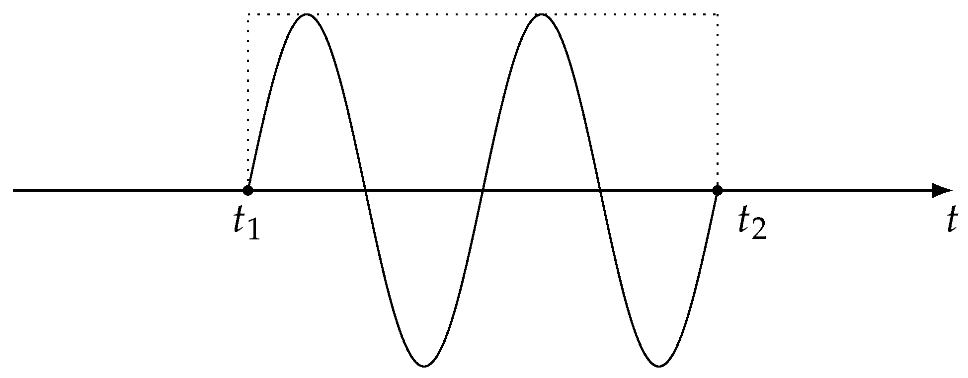
In the following, we assume that the optical dressing pulse has a rectangular shape:

$${\epsilon }_d\left(t\right)=A_d\left(\theta (t-t_1)-\theta (t-t_2)\right)\sin \left({\omega }_{d}t\right),$$

(19)

as shown in Figure 1.

In Equation (19), ${\omega }_d$ is the photon energy of the dressing field and $A_d$ is the field amplitude. The dressing pulse is assumed to start at $t_1=0$. Thus, the time $\tau$ associated with the attosecond XUV pulse is the delay of the attosecond XUV pulse relative to the beginning of the optical dressing pulse. For the pulse in Equation (19), analytical expressions can be obtained for the functions $f_{fxy0}^{mn}\left(t\right)$ appearing in Equation (18). These analytical expressions may be found in the appendix, where we assume that initial-state dressing is negligible, i.e., in Equation (18) terms involving indices a and b are set to zero.

From Equation (12) we see that the XUV one-photon cross-section can be written as:

$$\begin{array}{cc}\hfill {\sigma }^{\left(1\right)}(\omega ,\tau )& =\frac{2\pi \omega }{c}\sum _f\left({\tilde{F}}_{0f}(\omega ,\tau )F_{f0}\left(\tau \right)e^{-i\omega \tau }-{\tilde{F}}_{0f}(-\omega ,\tau )F_{f0}\left(\tau \right)e^{i\omega \tau }+c.c.\right),\hfill \end{array}$$

(20)

where

$${\tilde{F}}_{0f}(\omega ,\tau )=\underset{-\infty }{\overset{\infty }{\int }}dt{F}_{0f}\left(t\right)\theta (t-\tau )e^{i\omega t}$$

(21)

is the Fourier transform of the function $F_{0f}\left(t\right)\theta (t-\tau )$. In view of Equation (20), the analytical structure of ${\tilde{F}}_{0f}(\omega ,\tau )$ determines the resonance peaks in the XUV one-photon cross-section as a function of $\omega$. As shown in the appendix, ${\tilde{F}}_{0f}(\omega ,\tau )$ has the general form:

$${\tilde{F}}_{0f}(\omega ,\tau )=\sum _k{C}_k\frac{e^{-i({\Delta }_k-i\frac{{\mathrm{\Gamma }}_f}{2}-\omega )\tau }}{i({\Delta }_k-i\frac{{\mathrm{\Gamma }}_f}{2}-\omega )},$$

(22)

where each ${\Delta }_k$ is one of the quantities presented in Equations (A1)–(A3) in the appendix. Thus, the ${\Delta }_k$ define the poles of ${\tilde{F}}_{0f}(\omega ,\tau )$ in the complex $\omega$ plane. The peaks of ${\sigma }^{\left(1\right)}(\omega ,\tau )$ at the ${\Delta }_k$ correspond to XUV transitions accompanied by the absorption or emission of zero [Equation (A1)], one [Equation (A2)], or two [Equation (A3)] dressing-laser photons, or one absorption and one emission [Equation (A1)]. The $C_k$ in Equation (22) depend on whether the attosecond pulse precedes the dressing pulse ($-\infty <\tau <t_1$), whether the attosecond pulse overlaps with the dressing pulse ($t_1<\tau <t_2$), or whether the attosecond pulse arrives after the dressing pulse is over ($t_2<\tau <\infty$).

The coherent superposition of the electronically excited states associated with the resonance peaks at the energies ${\Delta }_k$ gives rise to oscillatory changes in the XUV one-photon cross-section as a function of $\tau$. To identify the associated frequencies, we take the Fourier transform of ${\sigma }^{\left(1\right)}(\omega ,\tau )$ with respect to the delay $\tau$ between the attosecond XUV pulse and the optical dressing pulse:

$${\tilde{\sigma }}^{\left(1\right)}(\omega ,{\omega }^{\prime })=\underset{-\infty }{\overset{\infty }{\int }}d\tau {\sigma }^{\left(1\right)}(\omega ,\tau )e^{i{\omega }^{\prime }\tau }.$$

(23)

From Equation (20) it follows that ${\tilde{\sigma }}^{\left(1\right)}(\omega ,{\omega }^{\prime })$ can be written as:

$${\tilde{\sigma }}^{\left(1\right)}(\omega ,{\omega }^{\prime })=\frac{2\pi \omega }{c}\sum _f\left(\widetilde{{\mathcal{F}}_f}(\omega ,{\omega }^{\prime })-\widetilde{{\mathcal{F}}_f}(-\omega ,{\omega }^{\prime })+{\tilde{\mathcal{F}}}_f^{\ast }(\omega ,-{\omega }^{\prime })-{\tilde{\mathcal{F}}}_f^{\ast }(-\omega ,-{\omega }^{\prime })\right),$$

(24)

where

$${\tilde{\mathcal{F}}}_f(\omega ,{\omega }^{\prime })=\underset{-\infty }{\overset{\infty }{\int }}d\tau {\tilde{F}}_{0f}(\omega ,\tau )F_{f0}\left(\tau \right)e^{i({\omega }^{\prime }-\omega )\tau }.$$

(25)

By making use of the analytical results provided in the appendix, one can see that the function ${\tilde{\mathcal{F}}}_f(\omega ,{\omega }^{\prime })$ has the following structure:

$${\tilde{\mathcal{F}}}_f(\omega ,{\omega }^{\prime })=\sum _{kj}\frac{A_{kj}(\omega ,{\omega }^{\prime })}{i({\Delta }_k-{\Delta }_j+{\omega }^{\prime })},$$

(26)

where the functions $A_{kj}(\omega ,{\omega }^{\prime })$ have no poles as a function of ${\omega }^{\prime }$. Therefore, the XUV one-photon cross-section ${\tilde{\sigma }}^{\left(1\right)}(\omega ,{\omega }^{\prime })$ has poles, as a function of ${\omega }^{\prime }$, at positions ${\Delta }_k-{\Delta }_j$, in which $\Delta$’s are combined in a way allowed by dipole selection rules. It is remarkable that some of these poles are entirely independent of the dressing-laser photon energy ${\omega }_d$, and some of the other poles depend only on ${\omega }_d$. We explore this in more detail in the following section.

3. Results for a Model Atom

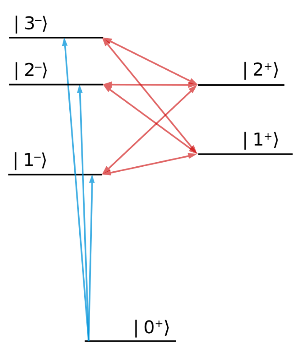
By focusing on a simple few-level atom, we perform in this section an analysis of the ATA signal dependence on the time decay between the attosecond XUV pulse and the optical dressing pulse. The model considered is shown in Figure 2.

The corresponding energy levels and transition dipole matrix elements, which underlie the numerical results shown in the following, are presented in

Table 1. Energy levels of the model atom.

${\mathbf{E}}_{0^{+}}$	${\mathit{E}}_{1^{-}}$	${\mathit{E}}_{2^{-}}$	${\mathit{E}}_{3^{-}}$	${\mathit{E}}_{1^{+}}$	${\mathit{E}}_{2^{+}}$
0	2.1888	2.2238	2.2360	2.1889	2.2238

and

Table 2. Transition dipole matrix elements $\langle i^{-}|\widehat{Z}|j^{+}\rangle$.

$\widehat{\mathit{Z}}$	$|0^{+}\rangle$	$|1^{+}\rangle$	$|2^{+}\rangle$
$\langle {\mathbf{1}}^{-}|$	0.25	0.33	0.33
$\langle {\mathbf{2}}^{-}|$	0.42	0.33	0.33
$\langle {\mathbf{3}}^{-}|$	0.33	0.33	0.33

, respectively.

The numbers employed do not correspond to any real atom. To illustrate the basic features of the kind of ATA spectroscopy considered in this paper, we employ an artificial few-level system characterized by level spacings matching XUV and optical energies. A key assumption is that parity is a good quantum number, which allows us to cleanly distinguish between bright and dark states (with respect to excitation from the ground state). The model in Figure 2 is intended as a pedagogical tool for identifying generic features of ${\sigma }^{\left(1\right)}(\omega ,\tau )$ and ${\tilde{\sigma }}^{\left(1\right)}(\omega ,{\omega }^{\prime })$.

As a consequence of its large spectral bandwidth, the attosecond XUV pulse can excite the atom from its ground state $0^{+}$ to any of the bright states $i^{-}$, $i=1,2,3$, which have a negative parity (see Figure 2). The dressing pulse with photon energy ${\omega }_d$ cannot, by assumption, affect the ground state, but can couple a bright state $i^{-}$ to a dark state $j^{+}$, by exchanging with the atom one dressing-laser photon (energy change by $\pm {\omega }_d$) or to a bright state $j^{-}$ by exchanging with the atom two dressing-laser photons (energy change by $\pm 2{\omega }_d$). Because $0^{+}$ and the dark states $j^{+}$, $j=1,2$, have the same parity (see Figure 2), the latter cannot be excited via one-photon absorption from the ground state (i.e., the corresponding transition dipole moments are zero); but in the presence of the dressing laser, they can give rise to light-induced states [52,53,54]. As a function of the XUV photon energy $\omega$, the following transition energies can be observed in the transmitted spectrum of the attosecond pulse: $E_{i^{-}}-E_{0^{+}}$ for a transition to a bright state $i^{-}$, and $E_{i^{+}}\pm {\omega }_d-E_{0^{+}}$ and $E_{i^{-}}\pm 2{\omega }_d-E_{0^{+}}$, respectively, for light-induced states (LIS). Excited states of the atom have a finite decay rate $\mathrm{\Gamma }={\mathrm{\Gamma }}_f$ and relax through fluorescence or Auger decay, which leads to a finite width of the absorption peaks. In our model, the decay rate $\mathrm{\Gamma }$ is assumed to be the same for all excited states $i^{+}$ and $i^{-}$ ($\mathrm{\Gamma }=1/263$ a.u.).

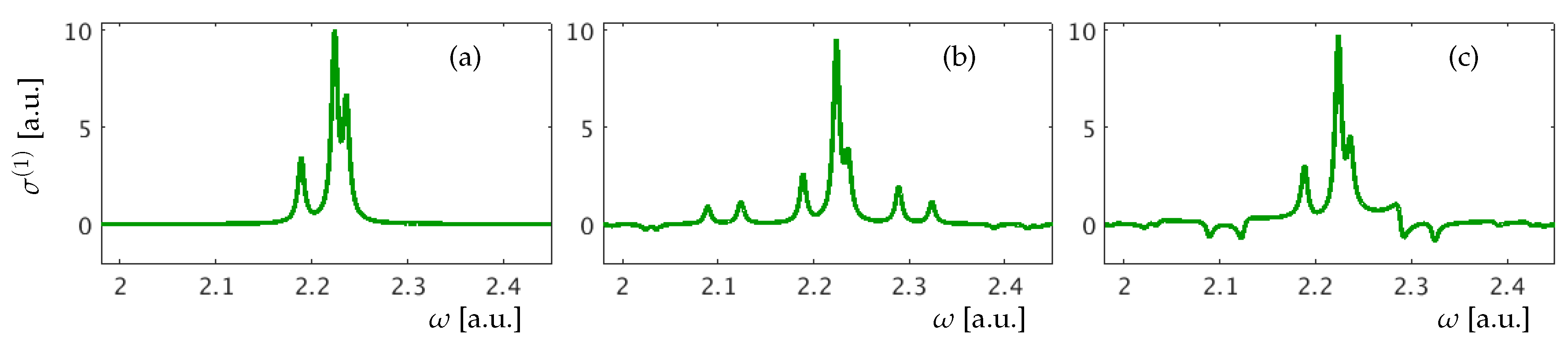
In Figure 3, the XUV one-photon cross-section ${\sigma }^{\left(1\right)}(\omega ,\tau )$ [Equation (12)] for our model atom is presented for three different time delays $\tau$.

In all figures below we use a dressing pulse with amplitude $A_d=0.06$ a.u., photon energy ${\omega }_d$ = 0.10 a.u. and duration $t_2=3141$ a.u. $\approx 11.95/\mathrm{\Gamma }$ a.u., unless stated otherwise. As there are three bright states $i^{-}$ in our model atom, one can see three main peaks in Figure 3, which correspond to the XUV transitions $0^{+}\to i^{-}$. The small additional peaks correspond to transitions to LIS. Numerical values for the transition energies are listed in

Table 3. Resonance energies (dressing photon energy ${\omega }_d$ = 0.10 a.u.).

	i = 1	i = 2	i = 3
${\mathit{E}}_{{\mathit{i}}^{-}}-{\mathit{E}}_{{\mathbf{0}}^{+}}-\mathbf{2}{\mathit{\omega }}_{\mathit{d}}$	1.9889	2.0238	2.0361
${\mathit{E}}_{{\mathit{i}}^{-}}-{\mathit{E}}_{{\mathbf{0}}^{+}}$	2.1888	2.2238	2.2360
${\mathit{E}}_{{\mathit{i}}^{-}}-{\mathit{E}}_{{\mathbf{0}}^{+}}+\mathbf{2}{\mathit{\omega }}_{\mathit{d}}$	2.3888	2.4238	2.4360
${\mathit{E}}_{{\mathit{i}}^{+}}-{\mathit{E}}_{{\mathbf{0}}^{+}}-{\mathit{\omega }}_{\mathit{d}}$	2.089	2.124
${\mathit{E}}_{{\mathit{i}}^{+}}-{\mathit{E}}_{{\mathbf{0}}^{+}}+{\mathit{\omega }}_{\mathit{d}}$	2.289	2.324

.

If dressing comes long after or before the excitation by the attosecond pulse, only the peaks associated with the bright states can be observed in the absorption spectrum (Figure 3a). When the time delay between the pulses gets shorter, optical dressing becomes possible, causing the appearance of LIS transition peaks as well as changes in the height of the bright-state transition peaks. New features can be positive or negative indicating whether the attosecond XUV beam is attenuated or amplified at the corresponding $\omega$.

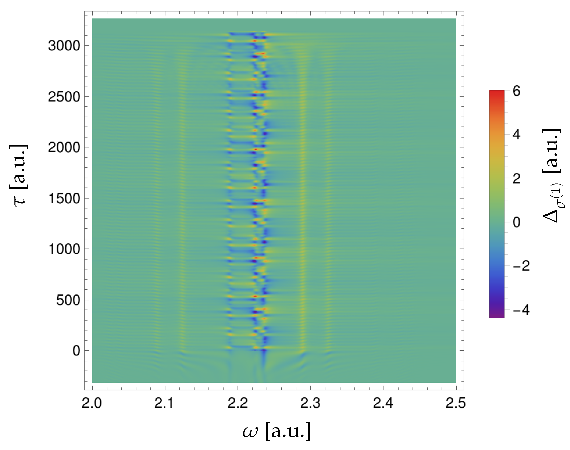
In Figure 4 we show the difference ${\Delta }_{{\sigma }^{\left(1\right)}}={\sigma }^{\left(1\right)}(\omega ,\tau )-{\sigma }^{\left(1\right)}(\omega ,\infty )$ as a function of $\omega$ and $\tau$.

Interference of different excitation paths from the ground state $0^{+}$ to a final f state [see Equation (12)] gives rise to an oscillation in the XUV one-photon cross-section of all peaks [55], which can be observed in Figure 4 in the overlap region between the optical dressing pulse and the attosecond XUV pulse. The oscillations become weaker after $\tau \approx 2230$ a.u. as the time available to dress an excited state gets shorter and becomes comparable with the excited-state lifetime. Thus, the probability of interference with another transition path through a dressed state goes down. This “ringing” of the system driven by the excitation pulse can be observed even if the dressing pulse comes after the excitation and the pulses do not overlap, if the excited state can survive till the dressing comes. This can be seen in the region of negative $\tau$ in Figure 4. If the attosecond pulse comes after the dressing pulse, the XUV one-photon cross-section remains constant and the height of the three main peaks at $E_{i^{-}}-E_{0^{+}}$ does not change with the time delay $\tau$, as the dressing pulse, by assumption, does not affect the ground state of the system.

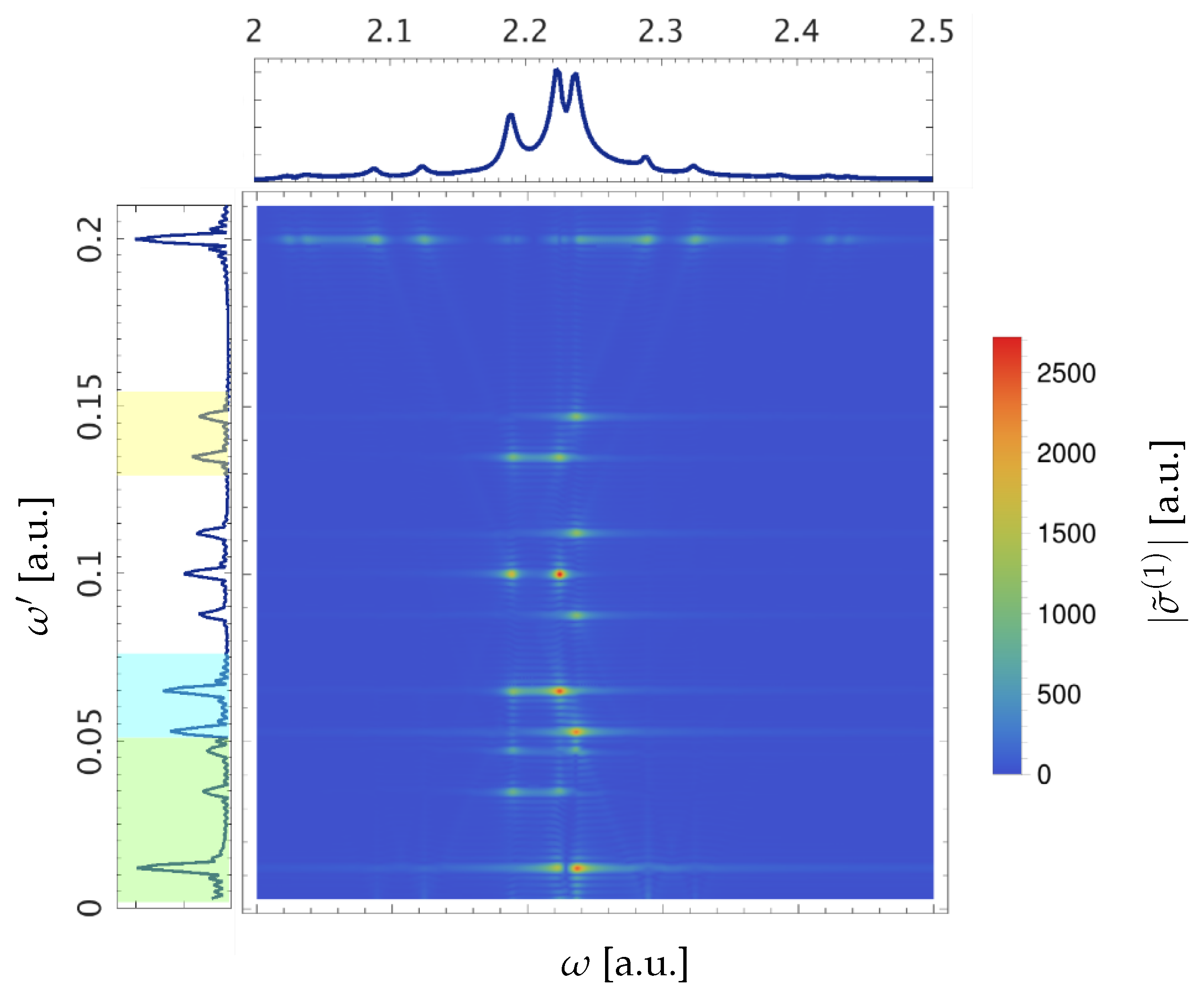
Studying the “ringing” allows us to reveal the real-time attosecond dynamics inside the atom. To this end, we take the Fourier transform of ${\sigma }^{\left(1\right)}(\omega ,\tau )$ with respect to the time delay, which gives an opportunity to study the reasons behind the oscillations observed. The absolute value of the resulting function ${\tilde{\sigma }}^{\left(1\right)}(\omega ,{\omega }^{\prime })$ [Equation (24)] is plotted in Figure 5.

The oscillations of ${\sigma }^{\left(1\right)}(\omega ,\tau )$, caused by the excitation path interference, have the energies ${\Delta }_i-{\Delta }_j$ (see Section 2.3). In accordance with the dipole selection rules, these are $2{\omega }_d$, $|E_{i^{-}}-E_{j^{-}}|$, $|E_{i^{+}}-E_{j^{-}}\pm {\omega }_d|$ (

Table 4. Oscillation energies ${\omega }^{\prime }$ [a.u.] of the ATA peaks, dependent on the electronic structure of the atom ($2{\omega }_d=0.20$ a.u. is missing in the table).

	i = 1	i = 2	i = 3
$|{\mathit{E}}_{{\mathit{i}}^{-}}-{\mathit{E}}_{{(\mathit{i}+\mathbf{1})}^{-}}|$	0.0350	0.0122	0.0472 ${}^{\ast }$
$|{\mathit{E}}_{{\mathbf{1}}^{+}}-{\mathit{E}}_{{\mathit{i}}^{-}}+{\mathit{\omega }}_{\mathit{d}}|$	0.1000	0.0650	0.0528
$|{\mathit{E}}_{{\mathbf{2}}^{+}}-{\mathit{E}}_{{\mathit{i}}^{-}}+{\mathit{\omega }}_{\mathit{d}}|$	0.1350	0.1000	0.0878
$|{\mathit{E}}_{{\mathbf{1}}^{+}}-{\mathit{E}}_{{\mathit{i}}^{-}}-{\mathit{\omega }}_{\mathit{d}}|$	0.0999	0.1350	0.1472
$|{\mathit{E}}_{{\mathbf{2}}^{+}}-{\mathit{E}}_{{\mathit{i}}^{-}}-{\mathit{\omega }}_{\mathit{d}}|$	0.0650	0.0999	0.1122

${}^{\ast }$Energy difference, $E_{3^{-}}-E_{1^{-}}$.

).

One can see all these energies in the oscillations of a main peak of the ATA spectrum, except those that do not include this concrete state in the interference process, such as ${\omega }^{\prime }=|E_{i^{-}}-E_{j^{-}}|$ for the absorption peak $\omega =|E_{k^{+}}-E_{0^{+}}|$, where $k\ne i$ and $k\ne j$. The first three peaks of the Fourier spectrum of the XUV one-photon cross-section (marked with a green color in the projection onto the ${\omega }^{\prime }$-axis in Figure 5) correspond to energy differences $|E_{i^{-}}-E_{j^{-}}|$, which appear due to coupling of two $i^{-}$ states by the dressing field. This makes it possible for the atom to be excited into the state $i^{-}$ with a following deexcitation from the $j^{-}$ state. In the middle of Figure 5 there are the peaks corresponding to ${\omega }^{\prime }=|E_{i^{-}}-E_{j^{+}}\pm {\omega }_d|$ energy differences. Oscillation energies marked in blue on the left in Figure 5 correspond to the coupling through or to the $1^{+}$ state for $2^{-}$ or $3^{-}$: ${\omega }^{\prime }=|E_{1^{+}}-E_{i^{-}}+{\omega }_d|$, $i=2,3$, and through or to the $2^{+}$ state for $1^{-}$: ${\omega }^{\prime }=|E_{2^{+}}-E_{1^{-}}-{\omega }_d|$. Analogously, in yellow are marked oscillation energies ${\omega }^{\prime }=|E_{1^{+}}-E_{i^{-}}-{\omega }_d|$ for $2^{-}$ and $3^{-}$, and ${\omega }^{\prime }=|E_{2^{+}}-E_{1^{-}}+{\omega }_d|$ for $1^{-}$. The remaining energies of this type correspond to ${\omega }^{\prime }=|E_{2^{+}}-E_{3^{-}}\pm {\omega }_d|$ are in the middle of the plot at the energies ${\omega }^{\prime }=0.087$ a.u. and ${\omega }^{\prime }=0.112$ a.u. The ${\omega }^{\prime }={\omega }_d=0.1\mathrm{a}.\mathrm{u}.$ oscillations appear due to the coupling of $1^{-}$ and $1^{+}$ or coupling of $2^{-}$ and $2^{+}$, whose energies were chosen rather close to each other. Oscillation at the energy ${\omega }^{\prime }=2{\omega }_d=0.2\mathrm{a}.\mathrm{u}.$ is characteristic for all cross-section peaks. This feature was theoretically predicted and measured as subcycle fringes in laser-dressed helium atoms [52,53,54]. It is noteworthy that the oscillation energy of these LIS peaks depends only on the photon energy of the dressing pulse and not on the electronic structure of the atom. In contrast, the energy ${\omega }^{\prime }=|E_{i^{-}}-E_{j^{-}}|$ of the main peaks’ oscillations does not depend on the energy of the dressing pulse at all, which testifies that the XUV excitation creates a coherent superposition of the $i^{-}$ states.

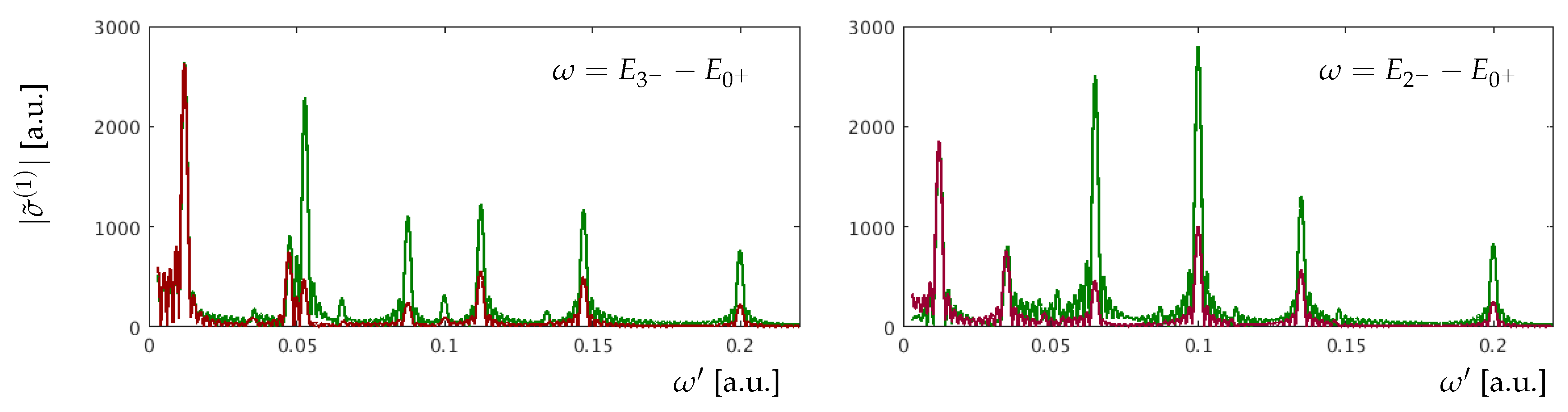
The intensity of a Fourier peak strongly depends on the atomic parameters as well as the pulse parameters. An important atomic parameter is the transition dipole matrix element between two states. In Figure 5 one can see that the Fourier peaks of the transition into $1^{-}$ are markedly weaker in comparison with $2^{-}$ and $3^{-}$, as the $1^{-}$ transition dipole matrix element from the ground state is smaller (Table 2) and as the energy gap between $1^{-}$ and the other two bright states is big. Moreover, our results obtained with Equation (24) show a sensitivity of ATA spectroscopy to the relative signs of the transition dipole matrix elements involved in the process. In Figure 6, we compare Fourier spectra of the oscillations of two different absorption peaks, where two cases are shown that differ from each other only through the sign of the transition dipole matrix element $\langle 3^{-}|\widehat{Z}|0^{+}\rangle$.

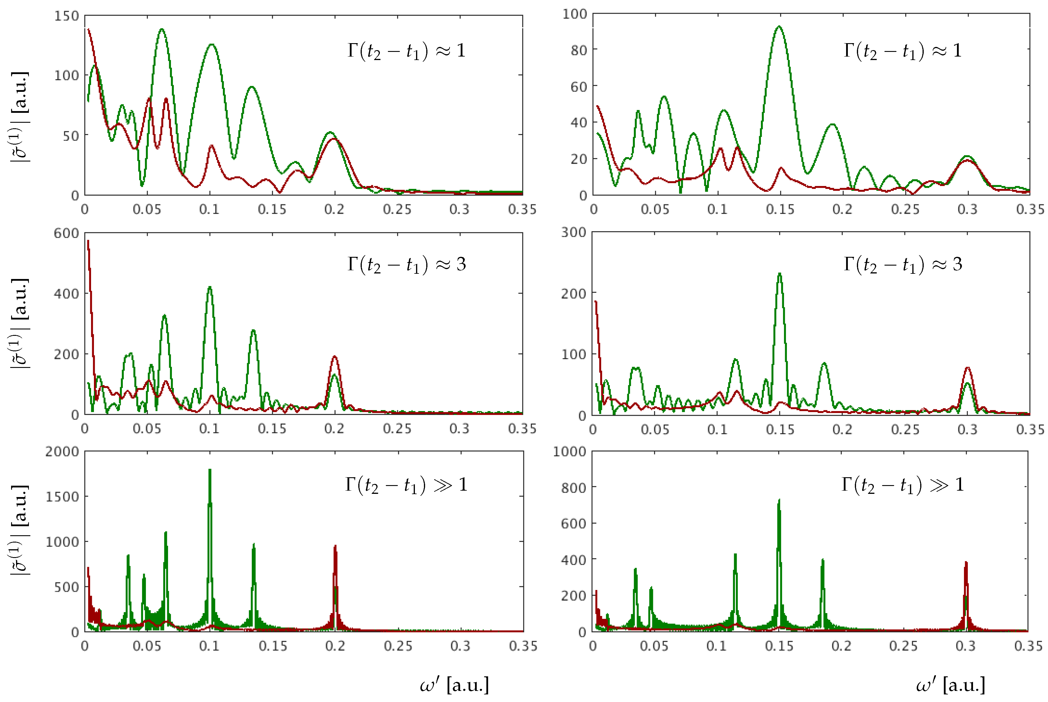
One can see significant changes in the amplitude of the Fourier peaks not only in the spectrum at $\omega =E_{3^{-}}-E_{0^{+}}$, which directly depends on parameters of the $3^{-}$ state, but also in the spectrum at $\omega =E_{2^{-}}-E_{0^{+}}$. This underscores the strong effective coupling between the $3^{-}$ and $2^{-}$ states. The change of the relative phase strongly affects the oscillation amplitudes that are explicitly dependent on transitions into LIS, whereas oscillations at the energies ${\omega }^{\prime }=E_{i^{-}}-E_{j^{-}}$ remain almost the same. The sensitivity to the relative phase, for transitions into LIS, can be understood as follows. If two bright states, here $2^{-}$ and $3^{-}$, are coupled by the dressing pulse to a dark state $j^{+}$, and the products $\langle 0^{+}|\widehat{Z}|2^{-}\rangle \langle 2^{-}|\widehat{Z}|j^{+}\rangle$ and $\langle 0^{+}|\widehat{Z}|3^{-}\rangle \langle 3^{-}|\widehat{Z}|j^{+}\rangle$ have opposite signs, then their contributions to the corresponding LIS peaks will attenuate each other. As a consequence of the destructive interference of the two pathways to the state $j^{+}$, the LIS peaks are suppressed. The impact of parameters of the dressing pulse is shown in Figure 7.

The panels show ${\tilde{\sigma }}^{\left(1\right)}(\omega ,{\omega }^{\prime })$ for the absorption peaks $\omega =E_{1^{-}}-E_{0^{+}}$ (green line) and $\omega =E_{1^{+}}-E_{0^{+}}+{\omega }_d$ (red line) calculated with Equation (24) for two different dressing photon energies ${\omega }_d=0.10$ a.u. (left panels) and ${\omega }_d=0.15$ a.u. (right panels) and different durations $t_2-t_1$ of the dressing pulse. Comparing the left and right panels of Figure 7 one can see that the peaks $E_{i^{-}}-E_{j^{-}}$ remain unaffected, and the peaks that depend on ${\omega }_d$ are shifted. As the effective coupling strength depends on the photon energy of the dressing field, the amplitudes of all peaks are affected by the ${\omega }_d$ change. The peak heights are sensitive to how close ${\omega }_d$ is to a resonant transition energy between the states $i^{-}$ and $j^{+}$. With increasing dressing pulse duration the relative heights of the peaks remain the same and all the peaks become sharp and clear.

4. Conclusions

We have presented an analytical theory of ATA spectroscopy for perturbatively dressed systems. This theory is applicable to the analysis of processes observed in pump-probe experiments if both pump and probe fields are sufficiently weak. We have used a two-stage approach based on perturbation theory, allowing us to give an analytical expression for the attosecond-resolved transient absorption signal.

In this work we have discussed an unusual kind of pump-probe experiment, where the information is gained from the absorption spectrum of an attosecond XUV pulse, which serves as a pump pulse at the same time. The optical probe pulse in this kind of experiment gives a reference time that provides a possibility to measure the time evolution of a system of interest. When a broadband attosecond XUV pulse excites a superposition of bright states, the presence of an optical dressing pulse gives rise to modulations of the absorption peaks connected to the population of bright states and, in addition, allows the population of LIS, which can be observed as new absorption lines in the ATA spectrum. Their positions depend on the energy of the dressing pulse. The modulations of the bright-state absorption peaks are caused by the dressing-laser-driven coherent coupling of the bright states to dark states and, via the dark states, to other bright states. The amplitude of a bright state excited by the attosecond XUV pulse can, thus, be enhanced or reduced via population transfer from or to other bright states by the dressing pulse. Therefore, the interference between the direct and the dressing-field-mediated pathways gives rise to periodic modulations of the bright-state absorption peaks as a function of the pump-probe delay. The energies associated with these modulations do not depend on the photon energy of the optical dressing pulse but on the energy differences among the bright states coherently populated by the attosecond XUV pulse.

The developed theory also shows the sensitivity of ATA spectroscopy to the relative signs of the transition dipole moments among the states involved in the interaction. A change in sign affects the interference of different quantum pathways, which can be observed via the strength of the corresponding modulations of an absorption peak. The presented technique is suitable not only for atoms, but for more complex systems as well.

References

- Tamai, N.; Miyasaka, H. Ultrafast dynamics of photochromic systems. Chem. Rev. 2000, 100, 1875–1890. [Google Scholar] [CrossRef] [PubMed]
- Joly, A.G.; Nelson, K.A. Femtosecond transient absorption spectroscopy of chromium hexacarbonyl in methanol: Observation of initial excited states and carbon monoxide dissociation. J. Phys. Chem. 1989, 93, 2876–2878. [Google Scholar] [CrossRef]
- Pfeifer, T.; Spielmann, C.; Gerber, G. Femtosecond X-ray science. Rep. Prog. Phys. 2006, 69, 443–505. [Google Scholar] [CrossRef]
- Zewail, A.H. Femtochemistry. Atomic-scale dynamics of the chemical bond. J. Phys. Chem. A 2000, 104, 5660–5694. [Google Scholar] [CrossRef]
- Dhar, L.; Rogers, J.A.; Nelson, K.A. Time-resolved vibrational spectroscopy in the impulsive limit. Chem. Rev. 1994, 94, 157–193. [Google Scholar] [CrossRef]
- Petek, H.; Ogawa, S. Femtosecond time-resolved two-photon photoemission studies of electron dynamics in metals. Prog. Surf. Sci. 1997, 56, 239–310. [Google Scholar] [CrossRef]
- Othonos, A. Probing ultrafast carrier and phonon dynamics in semiconductors. J. Appl. Phys. 1998, 83, 1789–1830. [Google Scholar] [CrossRef]
- Voisin, C.; Fatti, N.D.; Christofilos, D.; Vallee, F. Ultrafast electron dynamics and optical nonlinearities in metal nanoparticles. J. Phys. Chem. B 2001, 105, 2264–2280. [Google Scholar] [CrossRef]
- Stolow, A.; Bragg, A.E.; Neumark, D.M. Femtosecond time-resolved photoelectron spectroscopy. Chem. Rev. 2004, 104, 1719–1758. [Google Scholar] [CrossRef] [PubMed]
- Sokolowski-Tinten, K.; Von Der Linde, D. Ultrafast phase transitions and lattice dynamics probed using laser-produced X-ray pulses. J. Phys. Condens. Matter 2004, 16, R1517–R1536. [Google Scholar] [CrossRef]
- Güdde, J.; Höfer, U. Femtosecond time-resolved studies of image-potential states at surfaces and interfaces of rare-gas adlayers. Prog. Surf. Sci. 2005, 80, 49–91. [Google Scholar] [CrossRef]
- Nibbering, E.T.J.; Fidder, H.; Pines, E. Ultrafast chemistry: Using time-resolved vibrational spectroscopy for interrogation of structural dynamics. Annu. Rev. Phys. Chem. 2005, 56, 337–367. [Google Scholar] [CrossRef]
- Kukura, P.; McCamant, D.W.; Mathies, R.A. Femtosecond stimulated Raman spectroscopy. Annu. Rev. Phys. Chem. 2007, 58, 461–488. [Google Scholar] [CrossRef] [PubMed]
- Gühr, M.; Bargheer, M.; Fushitani, M.; Kiljunen, T.; Schwentner, N. Ultrafast dynamics of halogens in rare gas solids. Phys. Chem. Chem. Phys. 2007, 9, 779–801. [Google Scholar] [CrossRef] [PubMed]
- Sundstrom, V. Femtobiology. Annu. Rev. Phys. Chem. 2008, 59, 53–77. [Google Scholar] [CrossRef]
- Southworth, S.H.; Arms, D.A.; Dufresne, E.M.; Dunford, R.W.; Ederer, D.L.; Höhr, C.; Kanter, E.P.; Krässig, B.; Landahl, E.C.; Peterson, E.R.; et al. K-edge X-ray-absorption spectroscopy of laser-generated Kr+ and Kr2+. Phys. Rev. A 2007, 76, 043421. [Google Scholar] [CrossRef]
- Loh, Z.H.; Khalil, M.; Correa, R.E.; Santra, R.; Buth, C.; Leone, S.R. Quantum state-resolved probing of strong-field-ionized xenon atoms using femtosecond high-order harmonic transient absorption spectroscopy. Phys. Rev. Lett. 2007, 98, 143601. [Google Scholar] [CrossRef]
- Young, L.; Arms, D.A.; Dufresne, E.M.; Dunford, R.W.; Ederer, D.L.; Höhr, C.; Kanter, E.P.; Krässig, B.; Landahl, E.C.; Peterson, E.R.; et al. X-ray microprobe of orbital alignment in strong-field ionized atoms. Phys. Rev. Lett. 2006, 97, 083601. [Google Scholar] [CrossRef] [PubMed]
- Santra, R.; Dunford, R.W.; Young, L. Spin-orbit effect on strong-field ionization of krypton. Phys. Rev. A 2006, 74, 043403. [Google Scholar] [CrossRef]
- Johnsson, P.; Mauritsson, J.; Remetter, T.; L’Huillier, A.; Schafer, K.J. Attosecond control of ionization by wave-packet interference. Phys. Rev. Lett. 2007, 99, 233001. [Google Scholar] [CrossRef]
- Glover, T.E.; Hertlein, M.P.; Southworth, S.H.; Allison, T.K.; van Tilborg, J.; Kanter, E.P.; Krässig, B.; Varma, H.R.; Rude, B.; Santra, R.; et al. Controlling X-rays with light. Nat. Phys. 2009, 6, 69–74. [Google Scholar] [CrossRef]
- Ranitovic, P.; Tong, X.M.; Gramkow, B.; De, S.; DePaola, B.; Singh, K.P.; Cao, W.; Magrakvelidze, M.; Ray, D.; Bocharova, I.; et al. IR-assisted ionization of helium by attosecond extreme ultraviolet radiation. New J. Phys. 2010, 12, 013008. [Google Scholar] [CrossRef] [Green Version]
- Wickenhauser, M.; Burgdörfer, J.; Krausz, F.; Drescher, M. Time-resolved Fano resonances. Phys. Rev. Lett. 2005, 94, 023002. [Google Scholar] [CrossRef]
- Buth, C.; Santra, R.; Young, L. Electromagnetically induced transparency for X-rays. Phys. Rev. Lett. 2007, 98, 253001. [Google Scholar] [CrossRef]
- Pfeifer, T.; Abel, M.J.; Nagel, P.M.; Jullien, A.; Loh, Z.-H.; Bell, M.J.; Neumark, D.M.; Leone, S.R. Time-resolved spectroscopy of attosecond quantum dynamics. Chem. Phys. Lett. 2008, 463, 11–24. [Google Scholar] [CrossRef]
- Santra, R.; Buth, C.; Peterson, E.R.; Dunford, R.W.; Kanter, E.P.; Krässig, B.; Southworth, S.H.; Young, L. Strong-field control of X-ray absorption. J. Phys. Conf. Ser. 2007, 88, 012052. [Google Scholar] [CrossRef]
- Buth, C.; Santra, R. Theory of X-ray absorption by laser-dressed atoms. Phys. Rev. A 2007, 75, 033412. [Google Scholar] [CrossRef]
- Buth, C.; Santra, R. X-ray refractive index of laser-dressed atoms. Phys. Rev. A 2008, 78, 043409. [Google Scholar] [CrossRef]
- Porter, G.; Topp, M.R. Nanosecond flash photolysis and the absorption spectra of excited singlet states. Nature 1968, 220, 1228–1229. [Google Scholar] [CrossRef]
- Dantus, M.; Rosker, M.J.; Zewail, A.H. Real-time femtosecond probing of “transition states” in chemical reactions. J. Chem. Phys. 1987, 87, 2395–2397. [Google Scholar] [CrossRef]
- Bressler, C.; Chergui, M. Ultrafast X-ray absorption spectroscopy. Chem. Rev. 2004, 104, 1781–1812. [Google Scholar] [CrossRef]
- Chen, L.X. Probing transient molecular structures in photochemical processes using laser-initiated time-resolved X-ray absorption spectroscopy. Annu. Rev. Phys. Chem. 2005, 56, 221–254. [Google Scholar] [CrossRef]
- Seres, E.; Spielmann, C. Ultrafast soft X-ray absorption spectroscopy with sub-20-fs resolution. Appl. Phys. Lett. 2007, 91, 121919. [Google Scholar] [CrossRef]
- McPherson, A.; Gibson, G.; Jara, H.; Johann, U.; Luk, T.S.; McIntyre, I.A.; Boyer, K.; Rhodes, C.K. Studies of multiphoton production of vacuum-ultraviolet radiation in the rare gases. J. Opt. Soc. Am. B 1987, 4, 595–601. [Google Scholar] [CrossRef]
- Ferray, M.; L’Huillier, A.; Li, X.F.; Lompré, L.A.; Mainfray, G.; Manus, C. Multiple-harmonic conversion of 1064 nm radiation in rare gases. J. Phys. B 1988, 21, L31–L35. [Google Scholar] [CrossRef]
- Corkum, P.B. Plasma perspective on strong field multiphoton ionization. Phys. Rev. Lett. 1993, 71, 1994–1997. [Google Scholar] [CrossRef] [Green Version]
- Krause, J.L.; Schafer, K.J.; Kulander, K.C. High-order harmonic generation from atoms and ions in the high intensity regime. Phys. Rev. Lett. 1992, 68, 3535–3538. [Google Scholar] [CrossRef] [PubMed]
- Paul, P.M.; Toma, E.S.; Breger, P.; Mullot, G.; Augé, F.; Balcou, P.; Muller, H.G.; Agostini, P. Observation of a train of attosecond pulses from high harmonic generation. Science 2001, 292, 1689–1692. [Google Scholar] [CrossRef] [PubMed]
- Goulielmakis, E.; Loh, Z.-H.; Wirth, A.; Santra, R.; Rohringer, N.; Yakovlev, V.S.; Zherebtsov, S.; Pfeifer, T.; Azzeer, A.M.; Kling, M.F.; et al. Real-time observation of valence electron motion. Nature 2010, 466, 739–743. [Google Scholar] [CrossRef]
- Blättermann, A.; Ott, C.; Kaldun, A.; Ding, T.; Pfeifer, T. Two-dimensional spectral interpretation of time-dependent absorption near laser-coupled resonances. J. Phys. B 2014, 47, 124008. [Google Scholar] [CrossRef] [Green Version]
- Santra, R.; Yakovlev, V.S.; Pfeifer, T.; Loh, Z.-H. Theory of attosecond transient absorption spectroscopy of strong-field-generated ions. Phys. Rev. A 2011, 83, 033405. [Google Scholar] [CrossRef]
- Pabst, S.; Sytcheva, A.; Moulet, A.; Wirth, A.; Goulielmakis, E.; Santra, R. Theory of attosecond transient-absorption spectroscopy of krypton for overlapping pump and probe pulses. Phys. Rev. A 2012, 86, 063411. [Google Scholar] [CrossRef]
- Baggesen, J.C.; Lindroth, E.; Madsen, L.B. Theory of attosecond absorption spectroscopy in krypton. Phys. Rev. A 2012, 85, 013415. [Google Scholar] [CrossRef]
- Gallmann, L.; Herrmann, J.; Locher, R.; Sabbar, M.; Ludwig, A.; Lucchini, M.; Keller, U. Resolving intra-atomic electron dynamics with attosecond transient absorption spectroscopy. Mol. Phys. 2013, 111, 2243–2250. [Google Scholar] [CrossRef]
- Cao, W.; Warrick, E.R.; Neumark, D.M.; Leone, S.R. Attosecond transient absorption of argon atoms in the vacuum ultraviolet region: Line energy shifts versus coherent population transfer. New J. Phys. 2016, 18, 013041. [Google Scholar] [CrossRef]
- Wu, M.; Chen, S.; Camp, S.; Schafer, K.J.; Gaarde, M.B. Theory of strong-field attosecond transient absorption. J. Phys. B 2016, 49, 062003. [Google Scholar] [CrossRef] [Green Version]
- Mukamel, S.; Loring, R.F. Nonlinear response function for time-domain and frequency-domain four-wave mixing. J. Opt. Soc. Am. B 1986, 3, 595. [Google Scholar] [CrossRef]
- Marx, C.A.; Harbola, U.; Mukamel, S. Nonlinear optical spectroscopy of single, few, and many molecules: Nonequilibrium Green’s function QED approach. Phys. Rev. A 2008, 77, 022110. [Google Scholar] [CrossRef] [PubMed]
- Mukamel, S. Partially-time-ordered Schwinger-Keldysh loop expansion of coherent nonlinear optical susceptibilities. Phys. Rev. A 2008, 77, 023801. [Google Scholar] [CrossRef]
- Biggs, J.D.; Voll, J.A.; Mukamel, S. Coherent nonlinear optical studies of elementary processes in biological complexes: Diagrammatic techniques based on the wave function versus the density matrix. Philos. Trans. R. Soc. A 2012, 370. [Google Scholar] [CrossRef] [PubMed]
- Keldysh, L.V. Ionization in the field of a strong electromagnetic wave. Sov. Phys. JETP 1965, 20, 1307–1314. [Google Scholar]
- Beck, A.R.; Neumark, D.M.; Leone, S.R. Probing ultrafast dynamics with attosecond transient absorption. Chem. Phys. Lett. 2015, 624, 119–130. [Google Scholar] [CrossRef] [Green Version]
- Chen, S.; Bell, M.J.; Beck, A.R.; Mashiko, H.; Wu, M.; Pfeiffer, A.N.; Gaarde, M.B.; Neumark, D.M.; Leone, S.R.; Schafer, K.J. Light-induced states in attosecond transient absorption spectra of laser-dressed helium. Phys. Rev. A 2012, 86, 063408. [Google Scholar] [CrossRef]
- Chen, S.; Wu, M.; Gaarde, M.B.; Schafer, K.J. Quantum interference in attosecond transient absorption of laser-dressed helium atoms. Phys. Rev. A 2013, 87, 033408. [Google Scholar] [CrossRef]
- Paul, H. Interference and ‘which way’ information. Opt. Quantum Electron. 1996, 28, 1111–1127. [Google Scholar] [CrossRef]
Figure 1.
Rectangular-shaped dressing pulse that starts at time and ends at , which is an integer multiple of the period .
Figure 2.
Level structure of the few-level atom employed to illustrate ATA spectroscopy. XUV transitions from the ground state are shown in blue. Red arrows indicate laser dressing of the excited states. The superscripts represent the parity of each state.
Figure 3.
Atomic cross-section at (a) ; (b) ; (c) .
Figure 4.
Difference .
Figure 5.
, i.e., the modulus of the Fourier transform of the XUV one-photon cross-section , calculated with Equation (24).
Figure 6.
Fourier spectrum of the oscillations at the and peaks (green: ; red: ).
Figure 7.
Fourier spectra at (green line) and (red line) for different pulse durations of the dressing field ( is kept constant). The pulse durations used are integers of the dressing field period. Left and right panels correspond to the dressing photon energies = 0.10 a.u. and = 0.15 a.u., respectively.