Enhanced Digital Image Correlation Analysis of Ruptures with Enforced Traction Continuity Conditions Across Interfaces

Abstract

Accurate measurements of displacements around opening or interfacial shear cracks (shear ruptures) are challenging when digital image correlation (DIC) is used to quantify strain and stress fields around such cracks. This study presents an algorithm to locally adjust the displacements computed by DIC near frictional interfaces of shear ruptures, in order for the local stress fields to satisfy the continuity of tractions across the interface. In the algorithm, the stresses near the interface are extrapolated by local polynomials that are constructed using a constrained inversion. This inversion is such that the traction continuity (TC) conditions are satisfied at the interface while simultaneously matching the displacements produced by the DIC solution at the pixels closest to the center of the subset, where the DIC fields are more accurate. We apply the algorithm to displacement fields of experimental shear ruptures obtained using a local DIC approach and show that the algorithm produces the desired continuous traction field across the interface. The experimental data are also used to examine the sensitivity of the algorithm against different geometrical parameters related to construction of the polynomials in order to avoid artifacts in the stress field.

1. Introduction

Understanding the dynamics of shear rupture of interfaces is important for fields ranging from failure of composites and bimaterial structures, to earthquakes, car brakes, and even to pistons of internal combustion engines. Recent advances in high-speed camera technologies have enabled the development of an experimental setup that combines ultra-high-speed photography with digital image correlation (DIC) to quantify the behavior of propagating dynamic ruptures in the laboratory [1,2,3], including full-field measurements of displacements, velocities, strains, and stresses (Figure 1).

DIC is an optical technique used to determine the full-field deformation between a reference and a deformed image [4,5,6]. The correlation algorithms use either global or local approaches to compute the desired field quantities [7,8]. In global approaches, the pattern matching is performed over the entire domain of analysis, typically using the finite element method [9,10], which allows enforcing compatibility of the displacement field. In local approaches, the image matching is performed with small windows, or “subsets”, separated by a distance, referred to as “step”, which can be less than half a subset size, (i.e., subsets can overlap) [4,11,12]. A number of recent investigations have focused on evaluating the accuracy and resolution of DIC [13,14]. The full-field measurements enabled by DIC have been used in a wide range of applications [4,6]. However, standard DIC techniques cannot capture displacement discontinuities associated with cracks or ruptures, as they assume a continuous displacement field [4]. Various approaches have been proposed to analyze discontinuous displacement fields [15,16,17,18,19,20,21,22], but they generally entail the application of constraints with a theoretical interpretation of the fields. This limits the implementation of such approaches to cases where the theoretical assumptions are valid.

In a previous study on dynamic ruptures conducted using an experimental setup similar to that employed here, it was possible to capture the static displacements associated with dynamic ruptures, after these ruptures traversed a part of a fault, because a low-frame-rate camera with high resolution (i.e., 4 megapixels) was employed [23]. In that study, the discontinuous displacement field was accurately mapped by simply having subsets over the interface as the high resolution and low noise of the images allowed for the subset size to be relatively small compared to the image size, so that smearing of the displacement fields caused by having subsets across the interface was minimal. Generally, local DIC approaches that provide the solution up to half a subset from the interface may also be sufficient when tracking the quasi-static propagation and opening of tensile crack faces and the associated strain field, using a large field of views and high-resolution cameras. However, these correlation approaches are not possible when the subset size is large compared to the field of view (i.e., when using low-resolution cameras), such as our ultra-high-speed camera (which has a resolution of 250 × 400 pixels²) or high-resolution cameras, but with comparatively large subset sizes, situations typically arising in the study of dynamic problems [3]. To resolve the displacement discontinuities on the interface associated with the propagation of dynamic shear ruptures, the studies in [1,2,3] used the commercial DIC software Vic-2D (Correlated Solutions, Inc.) to separately correlate the domains above and below the interface. While standard local DIC methods calculate displacements up to half a subset away from the interface, the “fill boundary” algorithm of Vic-2D employed in [1,2,3] uses affine transformation functions to extrapolate the displacements from the center of the subset up to the interface. This enables the use of large subsets in each side of the interface, which are essential to overcoming the noise associated with ultra-high-speed photography and the analyzed rapid ruptures. An important limitation of this approach, however, is that the extrapolated displacements are less accurate than those obtained directly by the actual correlation, especially at pixels near the interface, which have the largest distance from the subset center. This leads to errors in the strains and stresses near the interface, which are obtained from the spatial derivatives of the displacement fields. In addition, the non-coupled correlation of the domains above and below the interface results in non-physical discontinuities in the tractions across the interface.

This study proposes a simple and fast method to supplement the DIC solution with a post-processing algorithm that enforces the continuity of normal and shear tractions across the interface. The algorithm uses a constrained inversion to construct local 2-D polynomials that satisfy traction continuity conditions at the interface while matching the displacements of pixels closer to the center of the subset, where the DIC solution is most accurate. The polynomials are then used to calculate all stress components near the interface. In Section 2, we describe the experimental setup, including the laboratory experiment, ultra-high-speed diagnostics, the digital image correlation approach, and the post-processing procedure to turn the displacement fields into strain and stress fields. In Section 3, we present the method to enforce traction continuity along the interface and study the effects of the parameters involved in this method on the full-field stresses, displacements and particle velocities. Implications for the analysis of friction using the stress fields produced by this approach and conclusions are given in Section 4 and Section 5, respectively.

2. Monitoring Dynamic Shear Ruptures in the Laboratory

The algorithm developed in this paper is a post-processing algorithm that is designed to enforce the continuity of stresses measured near frictional interfaces during experimental dynamic ruptures. This section briefly summarizes the experimental setup, diagnostics, image analysis, and numerical methods that are used to obtain the displacement, strain, and stress fields before using the algorithm. This setup is the evolution of the Caltech “ Laboratory Earthquake Setup ” developed by Rosakis and his co-workers over a span of 15 years [1,2,3,24,25,26,27,28,29]. A more detailed description of the current form of the setup is given in [3].

The presentation focuses on the analysis of experimental dynamic ruptures, but the algorithm can be used for a wider range of frictional experiments that involve image analysis. The same methodology can also be used for the analysis of opening, shear, and mixed-mode cracks at both coherent and incoherent (frictional) interfaces separating both similar and dissimilar solids. Such interfaces are common in nature (e.g., faults), and are also important to a variety of engineering problems involving composites and bi-materials.

2.1. The Laboratory Setup

The laboratory setup is designed to study the dynamics of shear ruptures propagating along preexisting inclined frictional interfaces via full-field measurements of displacements, velocities, strains, and stresses associated with the rupture (Figure 1). Two Homalite-100 quadrilateral plates with a frictional interface inclined at an angle α are loaded under uniaxial compression P (Figure 1), resulting in initial shear and normal stresses on the interface of τ₀ = Psin(α)cos(α) and σ₀ = Pcos² (α), respectively. The rupture is nucleated by a local pressure release provided by a rapid expansion of a NiCr wire filament due to an electrical discharge of Cordin 640 high-voltage capacitor (Cordin, Salt Lake City, UT, USA). A key aspect of the setup is that the low shear modulus of Homalite enables production of well-developed dynamic ruptures in samples of tens of centimeters.

Once the rupture initiates, a target area coated with a random black-speckle pattern is monitored using Shimadzu HPV-X ultra-high-speed camera system (Shimadzu, Kyoto, Japan), capable of recording up to 10 million frames per second, and Cordin 605 high-speed white-light source system with two light heads (Cordin, Salt Lake City, UT, USA) (Figure 1). In the experiment reported here, the camera recorded a sequence of 128 images of the patterns distorted by the propagating rupture, with a resolution of 400 × 250 pixels², at a temporal sampling of 2 million frames/second and an exposure time of 200 ns. Moreover, the HPV-X camera was equipped with a range of prime telephoto lenses, which allowed it to monitor fields of view of different sizes [3].

2.2. Digital Image Correlation to obtain Displacement Fields

We employed the local digital image correlation (DIC) software Vic-2D (Correlation Solutions Inc.) to analyze the sequence of images acquired with the HPV-X high-speed camera, and to produce evolving displacement maps, computed with respect to a selected reference configuration. In local approaches, the correlation is performed on local “subsets” separated by a distance, referred to as “step”, which can be less than half the subset size (i.e., subsets can overlap) [4,11,12]. The 2D-DIC algorithms provide the two in-plane displacement components at each subset center. A parametric study performed in [3] showed that a subset size of 41 pixels and step size of 1 are needed to accurately resolve the spatial and temporal features of dynamic ruptures. In order to capture the discontinuous displacement field across the interface, the correlation is performed separately for the domains above and below the interface. While standard local DIC approaches are able to produce the displacement map up to half a subset away from the interface, the “fill boundary” algorithm of Vic-2D uses affine transformation functions to extrapolate the displacements from the center of the subset up to the interface.

2.3. Post-Processing of the Displacement Fields

Prior to the computation of strain fields, we filtered high-frequency noise from the displacement fields using a non-local-means (NL-means) filter [23,30,31]. This filter enables the displacement fields to be smoothed, while maintaining the original signal pattern. An example of full-field displacement maps of a laboratory rupture obtained using high-speed photography, DIC analysis, and a non-local filter is given in Figure 1. To facilitate comparisons, we report the same experimental rupture discussed in [1,3], produced with an applied vertical load P = 23 MPa and inclination angle α = 29°, and monitored with a small field of view. This was a super-shear rupture propagating at a speed of 2200 m/s. Super-shear ruptures are interfacial ruptures whose tip propagates at speeds greater than the shear wave speed of the surrounding solid, as first observed in [24,26,32,33]. Note that the full-field maps are cropped and their size is slightly smaller than the reported field of view size. These displacement fields are used throughout the study to test the capability of new algorithms to enforce traction continuity (TC) at the interface.

Strains are computed from the filtered displacement fields using finite difference approximation. We employ a frame system x₁-x₂ parallel to the interface and use the central difference scheme for pixels away from the boundaries [23]:

$${\epsilon }_{11}\left(i,j,k\right)=\frac{u_1\left(i,j+1,k\right)-u_1\left(i,j-1,k\right)}{2 s}$$

(1)

$${\epsilon }_{22}\left(i,j,k\right)=\frac{u_2\left(i+1,j,k\right)-u_2\left(i-1,j,k\right)}{2 s}$$

(2)

$${\epsilon }_{12}\left(i,j,k\right)=\frac{1}{2}\left(\frac{u_1\left(i+1,j,k\right)-u_1\left(i-1,j,k\right)}{2 s}+\frac{u_2\left(i,j+1,k\right)-u_2\left(i,j-1,k\right)}{2 s}\right),$$

(3)

where $u_1\left(i,j,k\right)$ and $u_2\left(i,j,k\right)$ are the interface-parallel and interface-normal displacement components, respectively, for pixel $\left(i,j\right)$ and frame k, and s is the step size. Note that the displacements in Equations (1)–(3) are expressed in pixels. Second-order backward and forward difference schemes are used to compute strains at the pixels immediately above and below the interface, respectively [1,3].

The stress changes with respect to the reference configuration (before rupture) are computed from the strain fields using the standard plane-stress linear elastic constitutive equations:

$$\left[\begin{array}{c}\Delta {\sigma }_{11}\left(x_1,x_2,t\right)\\ \Delta {\sigma }_{22}\left(x_1,x_2,t\right)\\ \Delta {\sigma }_{12}\left(x_1,x_2,t\right)\end{array}\right]=\frac{E}{1-{\nu }^2}\left[\begin{array}{ccc}1& \nu & 0\\ \nu & 1& 0\\ 0& 0& 1-\nu \end{array}\right]\left[\begin{array}{c}{\epsilon }_{11}\left(x_1,x_2,t\right)\\ {\epsilon }_{22}\left(x_1,x_2,t\right)\\ {\epsilon }_{12}\left(x_1,x_2,t\right)\end{array}\right],$$

(4)

where E is the Young’s modulus and ν is Poisson’s ratio. The actual stresses are given by:

$$\begin{gathered} {\sigma }_{11}\left(x_1,x_2,t\right)={\sigma }_{11\left(0\right)}\left(x_1,x_2\right)+\Delta {\sigma }_{11}\left(x_1,x_2,t\right) \\ {\sigma }_{22}\left(x_1,x_2,t\right)={\sigma }_{22\left(0\right)}\left(x_1,x_2\right)+\Delta {\sigma }_{22}\left(x_1,x_2,t\right) \\ {\sigma }_{12}\left(x_1,x_2,t\right)={\sigma }_{12\left(0\right)}\left(x_1,x_2\right)+\Delta {\sigma }_{12}\left(x_1,x_2,t\right), \end{gathered}$$

(5)

where ${\sigma }_{11\left(0\right)}\left(x_1,x_2\right)$, ${\sigma }_{22\left(0\right)}\left(x_1,x_2\right)={\sigma }_0$, and ${\sigma }_{12\left(0\right)}\left(x_1,x_2\right)={\tau }_0$ are the pre-stresses at the reference configuration. Since Homalite-100 is a strain-rate sensitive material at the strain rate levels developed during these dynamic ruptures, we use the dynamic values of the elastic constants to compute the stress changes [1,3]. An example of full-field maps of normal and shear stresses calculated from the displacement fields shown in Figure 1 are given in Figure 2a,b, respectively. The figures clearly show that the experimental technique enables capturing the spatial and temporal features of the ruptures. In particular, the more compressional and dilatational regions surrounding the crack are clearly imaged, as expected for shear ruptures (see [1,3] for more examples and physical insight). However, a significant limitation is that in the “fill boundary” algorithm of Vic-2D the domains above and below the interface are correlated and extrapolated towards the interface independently, without applying continuity constraints along the interface. Therefore, tractions are discontinuous at the interface, especially the normal component, where at some locations there is a difference of about 9 MPa between the normal tractions above and below the interface. Note that the increase of normal tractions towards the interface is the physical consequence of the shear rupture; however, close to the interface the tractions need to evolve towards being continuous. In the following section we present a post-processing algorithm to resolve this issue.

3. A Post-Processing Algorithm to Enforce Traction Continuity along the Interface

We present a method to supplement the DIC solution with a post-processing algorithm in which the displacements are modified in the proximity of the interface, such that the normal and shear tractions are continuous across the interface. The main idea is (i) to keep the displacement fields obtained with the local DIC up (or close) to the center of the subset touching the interface, and (ii) to use a portion of those fields to construct a polynomial extrapolation for the displacement so that stresses computed from the extrapolated displacements satisfy traction continuity conditions at the interface. The formulation presented here is for a coordinate frame x₁-x₂, such that x₁ is parallel to the interface. However, the method can easily be extended to any other frame. The procedure is described here for a given column of pixels at a given frame, and was implemented for all the columns and frames.

3.1. Traction Continuity Conditions

The condition for continuity of normal traction across the interface is given by

$${\sigma }_{22\left(0\right)}{}^{0+}+\Delta {\sigma }_{22}{}^{0+}={\sigma }_{22\left(0\right)}{}^{0-}+\Delta {\sigma }_{22}{}^{0-},$$

(6)

where the superscripts (⁰⁺) and (⁰⁻) denote the values immediately above and below the interface, respectively, and ${\sigma }_{22\left(0\right)}{}^{0+}={\sigma }_{22\left(0\right)}{}^{0-}$ are the initial stresses. Assuming a linear elastic response for the materials above and below the interface, the condition in Equation (6) can be written in terms of strains as

$$\frac{E^{+}}{1-{\nu }^{+}{}^2}\left({\epsilon }_{22}{}^{0+}+{\nu }^{+}{}_1{\epsilon }_{11}{}^{0+}\right)=\frac{E^{-}}{1-{\nu }^{-}{}^2}\left({\epsilon }_{22}{}^{0-}+{\nu }^{-}{\epsilon }_{11}{}^{0-}\right),$$

(7)

where the superscripts (⁺) and (⁻) denote the material properties above and below the interface, respectively. For small strains the condition can be expressed in terms of displacement gradients as

$$\frac{E^{+}}{1-{\nu }^{+}{}^2}\left({\frac{\partial u_2}{\partial x_2}}^{0+}+{\nu }^{+}{\frac{\partial u_1}{\partial x_1}}^{0+}\right)=\frac{E^{-}}{1-{\nu }^{-}{}^2}\left({\frac{\partial u_2}{\partial x_2}}^{0-}+{\nu }^{-}{\frac{\partial u_1}{\partial x_1}}^{0-}\right).$$

(8)

Similarly, the continuity of shear traction is expressed via

$${\sigma }_{12\left(0\right)}{}^{0+}+\Delta {\sigma }_{12}{}^{0+}={\sigma }_{12\left(0\right)}{}^{0-}+\Delta {\sigma }_{12}{}^{0-},$$

(9)

and

$${\mu }^{+}\left({\frac{\partial u_1}{\partial x_2}}^{0+}+{\frac{\partial u_2}{\partial x_1}}^{0+}\right)={\mu }^{-}\left({\frac{\partial u_1}{\partial x_2}}^{0-}+{\frac{\partial u_2}{\partial x_1}}^{0-}\right),$$

(10)

where $\mu$ is the shear modulus.

3.2. Approximating the Displacements with Local Polynomials

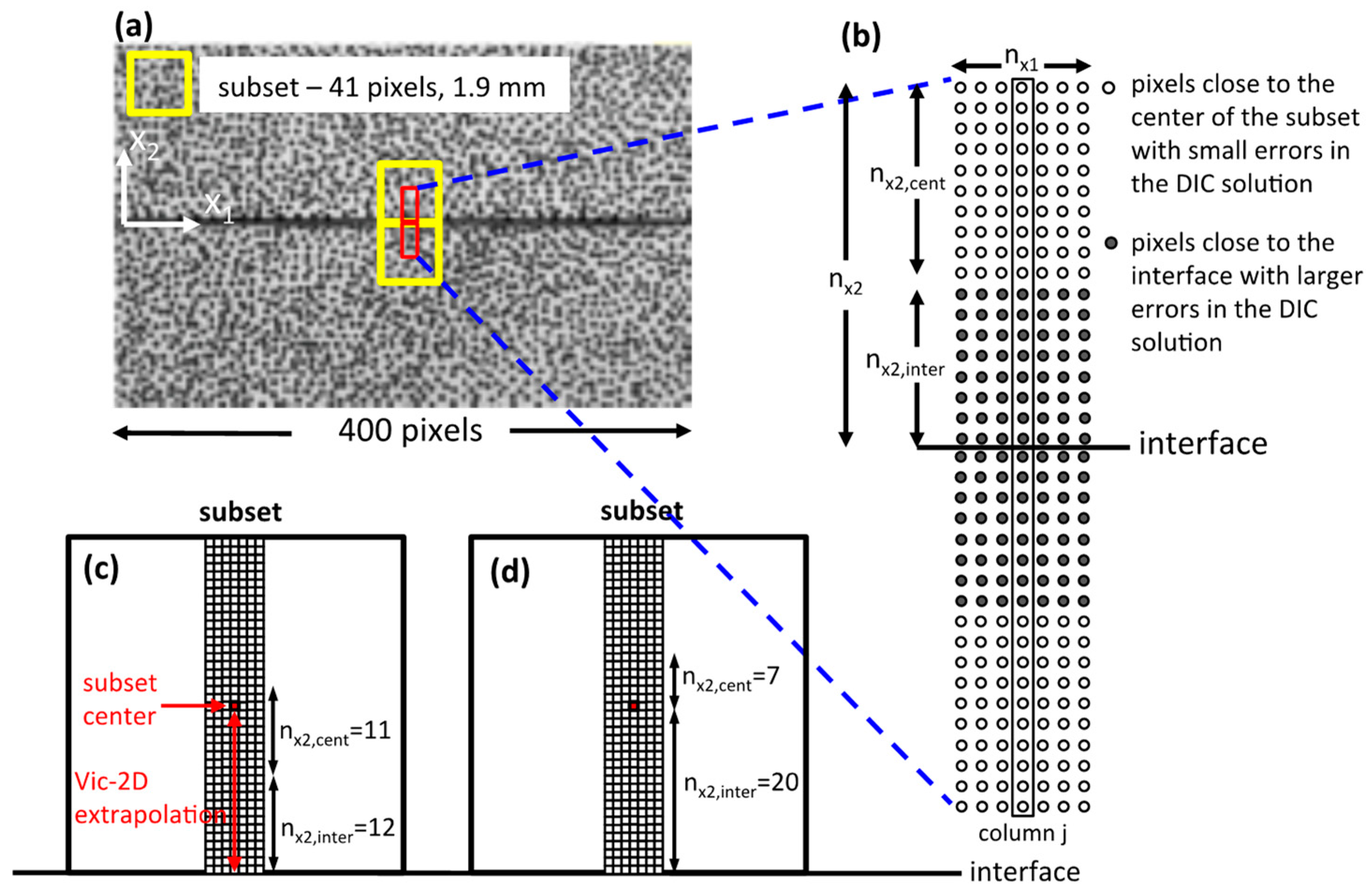
In order to modify the displacements near the interface for the jth column of pixels, we approximate the displacement fields $u_2^{+}$, $u_1^{+}$, $u_2^{-}$, and $u_1^{-}$ with local polynomials in terms of both spatial coordinates. The polynomials are defined over rectangles of $n_{x1}\times n_{x2}$ pixels above and below the interface, which are centered at the jth column of pixels (Figure 3). The pixels within each rectangle are divided into a group of $n_{x1}\times n_{x2,inter}$ pixels that are closer to the interface, and a group of $n_{x1}\times n_{x2,cent}$ pixels that are closer to the center of the subset. To represent the spatial variations in stresses, we approximate the displacement fields with cubic polynomials with n = 10 coefficients as

$$\begin{array}{l}\begin{array}{l}{u}_2^{p+}\left(x_1,x_2\right)=a_2^{10+}{x}_1{}^3+a_2^{9+}{x}_1{}^2{x}_2+a_2^{8+}{x}_1{}^2+a_2^{7+}{x}_1{x}_2{}^2+a_2^{6+}{x}_1{x}_2+a_2^{5+}{x}_1+a_2^{4+}{x}_2{}^3+a_2^{3+}{x}_2{}^2\\ +a_2^{2+}{x}_2+a_2^{1+}\end{array}\\ u_1^{p+}\left(x_1,x_2\right)=a_1^{10+}{x}_1{}^3+\cdots +a_1^{1+}\\ u_2^{p-}\left(x_1,x_2\right)=a_2^{10-}{x}_1{}^3+\cdots +a_2^{1-}\\ u_1^{p-}\left(x_1,x_2\right)=a_1^{10-}{x}_1{}^3+\cdots +a_1^{1-}\end{array}.$$

(11)

Note that $n_{x1}$ and $n_{x2}$ should be chosen small enough to avoid smoothing local patterns in the displacement fields.

3.3. Inverting for the Polynomial Coefficients

To obtain the polynomial coefficients, we aim to minimize the misfit between the observed displacements ${\mathrm{u}}_2^{ob+}$, ${\mathrm{u}}_2^{ob-}$, ${\mathrm{u}}_1^{ob+}$, and ${\mathrm{u}}_1^{ob-}$, produced by the DIC analysis, and the displacements predicted by the polynomials ${\mathrm{u}}_2^{p+}$, ${\mathrm{u}}_2^{p-}$, ${\mathrm{u}}_1^{p+}$, and ${\mathrm{u}}_1^{p-}$ at the pixels closer to the center of the subset. Recall that the DIC solution is computed up to half a subset away from the interface and extrapolated to the interface by the “fill Boundary” algorithm of Vic-2D. Since we expect such extrapolation to be reliable close to the center of the subset, but not close to the interface, we can use some of the extrapolated values by taking $n_{\mathrm{x}2,\mathrm{inter}}<20$ (Figure 3c). We can also exclude the displacement extrapolated by Vic-2D and consider only the computed values (up to the subset center) by taking $n_{\mathrm{x}2,\mathrm{inter}}\ge 20$ (Figure 3d). The minimization condition leads to the following system of equations:

$$\left[\left[\begin{array}{cccc}{\mathrm{X}}_{\left[\mathrm{m}\times \mathrm{n}\right]}^{+}& \cdots & \cdots & 0\\ ⋮& {\mathrm{X}}_{\left[\mathrm{m}\times \mathrm{n}\right]}^{-}& \ddots & ⋮\\ ⋮& \ddots & {\mathrm{X}}_{\left[\mathrm{m}\times \mathrm{n}\right]}^{+}& ⋮\\ 0& \cdots & \cdots & {\mathrm{X}}_{\left[\mathrm{m}\times \mathrm{n}\right]}^{-}\end{array}\right]\begin{array}{c}{\mathrm{A}}_{2\left[n\right]}^{+}\\ {\mathrm{A}}_{2\left[n\right]}^{-}\\ {\mathrm{A}}_{1\left[n\right]}^{+}\\ {\mathrm{A}}_{1\left[n\right]}^{-}\end{array}\right]=\left[\begin{array}{c}{\mathrm{u}}_{2\left[m\right]}^{ob+}\\ {\mathrm{u}}_{2\left[m\right]}^{ob-}\\ {\mathrm{u}}_{1\left[m\right]}^{ob+}\\ {\mathrm{u}}_{1\left[m\right]}^{ob-}\end{array}\right]$$

(12)

where

$${\mathrm{X}}_{\left[\mathrm{m}\times \mathrm{n}\right]}^{+}=\left[\begin{array}{cccc}{x}_{11}{}^3& x_{11}{}^2{x}_{12}& \cdots & 1\\ ⋮& ⋮& \ddots & ⋮\\ x_{m1}{}^3& x_{m1}{}^2{x}_{m2}& \cdots & 1\end{array}\right], x_2>0$$

and

$${\mathrm{X}}_{\left[\mathrm{m}\times \mathrm{n}\right]}^{-}=\left[\begin{array}{cccc}{x}_{11}{}^3& x_{11}{}^2{x}_{12}& \cdots & 1\\ ⋮& ⋮& \ddots & ⋮\\ x_{m1}{}^3& x_{m1}{}^2{x}_{m2}& \cdots & 1\end{array}\right], x_2<0$$

are the sensitivity sub-matrices above and below the interface, respectively,

$$\begin{gathered} {\mathrm{A}}_{2\left[n\right]}^{+}={\left[\begin{array}{ccc}{a}_2^{10+}& \cdots & a_2^{1+}\end{array}\right]}^T \\ {\mathrm{A}}_{2\left[n\right]}^{-}={\left[\begin{array}{ccc}{a}_2^{10-}& \cdots & a_2^{1-}\end{array}\right]}^T \\ {\mathrm{A}}_{1\left[n\right]}^{+}={\left[\begin{array}{ccc}{a}_1^{10+}& \cdots & a_1^{1+}\end{array}\right]}^T \\ {\mathrm{A}}_{1\left[n\right]}^{-}={\left[\begin{array}{ccc}{a}_1^{10-}& \cdots & a_1^{1-}\end{array}\right]}^T \end{gathered}$$

are the assemblies of polynomial coefficients, and $m=n_{x1}\times n_{x2,cent}$ is the number of pixels within the group closer to the center of the subset.

The polynomials must also fulfill the constraints for continuity of tractions across the interface. The condition for continuity of normal tractions is enforced by

$$\frac{E^{+}}{1-{\nu }^{+}{}^2}\left(\frac{\partial {\mathrm{u}}_2^{p0+}}{\partial x_2}+{\nu }^{+}\frac{\partial {\mathrm{u}}_1^{p0+}}{\partial x_1}\right)=\frac{E^{-}}{1-{\nu }^{-}{}^2}\left(\frac{\partial {\mathrm{u}}_2^{p0-}}{\partial x_2}+{\nu }^{-}\frac{\partial {\mathrm{u}}_1^{p0-}}{\partial x_1}\right)$$

(13)

and can be assembled into the following matrix form:

$$[\frac{E^{+}}{1-{\nu }^{+}{}^2}\frac{\partial {\mathrm{X}}_{\left[{\mathrm{n}}_{x1}\times \mathrm{n}\right]}^{0+}}{\partial x_2}\hspace{1em}-\frac{E^{-}}{1-{\nu }^{-}{}^2}\frac{\partial {\mathrm{X}}_{\left[{\mathrm{n}}_{x1}\times \mathrm{n}\right]}^{0-}}{\partial x_2}\hspace{1em}\frac{E^{+}}{1-{\nu }^{+}{}^2}\nu \frac{\partial {\mathrm{X}}_{\left[{\mathrm{n}}_{x1}\times \mathrm{n}\right]}^{0+}}{\partial x_1}\hspace{1em}-\frac{E^{-}}{1-{\nu }^{-}{}^2}\nu \frac{\partial {\mathrm{X}}_{\left[{\mathrm{n}}_{x1}\times \mathrm{n}\right]}^{0-}}{\partial x_1}]\left[\begin{array}{c}{\mathrm{A}}_{2,\left[n\right]}^{+}\\ {\mathrm{A}}_{2,\left[n\right]}^{-}\\ {\mathrm{A}}_{1,\left[n\right]}^{+}\\ {\mathrm{A}}_{1,\left[n\right]}^{-}\end{array}\right]=0,$$

(14)

where, for example,

$$\frac{\partial {\mathrm{u}}_2^{p0+}}{\partial x_2}=\frac{\partial {\mathrm{X}}_{\left[{\mathrm{n}}_{x1}\times \mathrm{n}\right]}^{0+}}{\partial x_2}{\mathrm{A}}_{2,\left[n\right]}^{+}=\left[\begin{array}{cccc}0& x_{11}{}^2& \cdots & 0\\ ⋮& ⋮& \ddots & ⋮\\ 0& x_{{\mathrm{n}}_{x1}1}{}^2& \cdots & 0\end{array}\right]{\mathrm{A}}_{2,\left[n\right]}^{+}, x_2=0.$$

Similarly, the condition for continuity of shear stresses is enforced by

$$\left[\begin{array}{cccc}{\mu }^{+}\frac{\partial {\mathrm{X}}_{\left[{\mathrm{n}}_{x1}\times \mathrm{n}\right]}^{0+}}{\partial x_1}& -{\mu }^{-}\frac{\partial {\mathrm{X}}_{\left[{\mathrm{n}}_{x1}\times \mathrm{n}\right]}^{0-}}{\partial x_1}& {\mu }^{+}\frac{\partial {\mathrm{X}}_{\left[{\mathrm{n}}_{x1}\times \mathrm{n}\right]}^{0+}}{\partial x_2}& -{\mu }^{-}\frac{\partial {\mathrm{X}}_{\left[{\mathrm{n}}_{x1}\times \mathrm{n}\right]}^{0-}}{\partial x_2}\end{array}\right]\left[\begin{array}{c}{\mathrm{A}}_{2,\left[n\right]}^{+}\\ {\mathrm{A}}_{2,\left[n\right]}^{-}\\ {\mathrm{A}}_{1,\left[n\right]}^{+}\\ {\mathrm{A}}_{1,\left[n\right]}^{-}\end{array}\right]=0.$$

(15)

Different methods can be used to solve the system of equations in Equation (12) together with the constraints in Equations (14) and (15) for the polynomial coefficients; here we use Matlab (The MathWorks, Natick, MA, USA) function lsqlin. Once the coefficients are obtained, the displacements at the pixels of the central column ($n_{x2}$ pixels above and $n_{x2}$ pixels below the interface) are replaced by those predicted by the corresponding polynomials, and the procedure is repeated for all columns and images. Note that the system of equations to be solved is small because the local polynomials should represent the local variations in displacements and stresses well. Thus, the computation time was small, and the modification of all pixel columns within an image was done within 2–3 s for the images analyzed here (400 pixels along the interface). Figure 4 shows the interface-parallel (a) and normal (b) displacements at the center of the field of view (j = 190) for the rupture of Figure 1. Both the displacements obtained by Vic-2D (with the “fill boundary” algorithm) and displacements modified by TC enforcement are shown. The maximum difference in displacements between the two solutions was smaller than 0.001 pixels, which is equivalent to 0.5% for u₁ and 1.5% for u₂, but it was enough to enforce the continuity of traction.

When the gradients in displacements in the direction parallel to the interface are large, as in the case of the rupture analyzed in this study, direct calculation of strains and stresses using the modified displacement fields may not result in completely continuous tractions at the interface. The calculation of strains and stresses for pixels in column j involves the displacements in columns j−1 and j + 1, as it requires displacement gradients with respect to x₁ (Equations (1)–(4)). When enforcing TC, these gradients are computed using the polynomial centered at column j. Once the displacement fields have been updated using the procedure described above, strains can be computed from the updated displacement fields, using finite difference schemes, as discussed in Section 2.3. However, the finite differences would be using the displacements of columns j−1 and j + 1, which are obtained from other polynomials than that used to enforce TC, those centered in columns j−1 and j + 1. As such, the spatial derivatives of the modified displacement field with respect to x₁ would be slightly different than those obtained during the enforcement of TC, using the polynomial centered at column j. Although the differences between polynomials centered at two neighboring columns are small, they may be enough to cause some discontinuities in tractions at the interface. To ensure the continuity of tractions, we computed strains and stresses within the $2\times n_{\mathrm{x}2}$ band, where displacements are updated directly as the algorithm goes over each column of pixels (i.e., we calculated the displacement derivatives for column j with respect to x₁ using the displacements in columns j−1 and j + 1 obtained from the polynomial centered at column j. Full-field maps of stresses modified by the algorithm using n_x1 = 7, n_x2,inter = 12, and n_x2,cent = 11 (Figure 2c,d) demonstrated the capability of this approach to generate more realistic and continuous stress fields near the interface. Interestingly, because of the symmetry of the problem, the enforcement of TC led to normal stresses that are close to the background value (∼17.6 MPa) at the interface.

3.4. The Effects of the Geometrical Parameters of the Polynomial

It is important to choose appropriate values for the geometrical parameters n_x1, n_x2,inter, and n_x2,cent in order not to introduce unwanted field distortions. For instance, a choice of a small value of n_x2,inter together with a large value of n_x2,cent or vice versa can lead to stress fields that are continuous on the interface, but have sharp discontinuities (Figure 2e,f) or spurious oscillations (Figure 2g,h) in the bulk. In this section, we study the effects of different parameter combinations in more details, aiming to find the parameter sets that avoid these distortions in the stress field. We ran the algorithm 324 times, varying the geometrical parameters in the following ranges: 3 ≤ n_x1 ≤ 9, 4 ≤ n_x2,inter ≤ 20, and 5 ≤ n_x2,cent ≤ 21. Note that for n_x1 ≥ 13 the system was over constrained. Overall, we found that parameters in ranges of 8 ≤ n_x2,inter ≤ 14 (1/5 to 1/3 of the subset size) and 7 ≤ n_x2,cent ≤ 15 gave similar results, independent of the value of n_x1.

We found that the stress fields obtained with the algorithm were insensitive to the value of n_x1. For example, there was no observable difference between full-field maps of stresses obtained with n_x1 = 3 and n_x1 = 9 (Figure 5a–d). To further examine the effect of n_x1, we plot the normal and shear stresses vs position along two lines perpendicular to the interface at x₁ = 170 and 220 pixels (Figure 5e–h). For both lines there was a “jump” larger than 5.5 MPa in the normal stress at the interface when the calculation was done with the “fill boundary” algorithm of Vic-2D without TC enforcement. The TC algorithm enforced the normal stress to be continuous across the interface, with a normal stress at the interface that was about the average of the normal stresses at the pixels immediately above and below the interface when TC was not enforced. The results were not sensitive to n_x1. A small effect of n_x1 on the shear stress was observed for the line located at x1 = 220 pixels (Figure 5h), with a difference of 0.12 MPa between the results for n_x1 = 3 and 9. The shear stress at the interface when TC was enforced were smaller than the shear stresses at the pixels immediately above and below the interface when TC was not enforced.

As shown in Figure 2e–h, a large difference between the parameters n_x2,inter and n_x2,cent resulted in artifacts in the stress field. On the one hand, taking n_x2,inter = 4 and n_x2,cent = 21 (with n_x1 = 7) resulted in discontinuities at the boundary between the Vic-2D solution and polynomial extrapolation (Figure 2e,f), n_x2,inter + n_x2,cent pixels away from the interface due to a poor fit between the stresses obtained by the polynomial and the original stresses at this region. On the other hand, taking n_x2,inter = 20 and n_x2,cent = 5 (with n_x1 = 7) resulted in spurious oscillations (Figure 2g,h). Some effects of n_x2,inter were observed also when n_x2,cent was fixed at a moderate value (e.g., n_x2,cent = 11), especially for the shear stress. A small value of n_x2,inter (e.g., n_x2,inter = 6) led to large gradients in the normal stresses near the interface, as well as to small discontinuities at the pixels located n_x2 pixels above and below the interface (Figure 6a,b). A large value of n_x2,inter (e.g., n_x2,inter = 16) resulted in an artificial increase or decrease of stresses at localized regions around the interface compared with the domains above and below (Figure 6c,d). For example, the normal stress decreased locally at the interface at x₁ = 370 pixels (Figure 6c), while the shear stress increased locally at x₁ = 170 and 370 pixels (Figure 6d). Some issues are illustrated further in plots of the normal and shear stresses vs position along two lines perpendicular to the interface at x₁ = 170 and 220 pixels (Figure 6e–h). The value of normal stress on the interface was similar for n_x2,inter ≤ 14, but diverged for higher values, with a difference of about 1 MPa for n_x2,inter = 20. For n_x2,inter ≤ 6, the TC enforcement resulted in a poor agreement between the stresses obtained by the polynomial and the original stresses also at the pixels closer to the center of the subset. The shear stress at the interface also diverged, with an increase of about 1 MPa for n_x2,inter = 16, at x₁ = 170 pixels (Figure 6f).

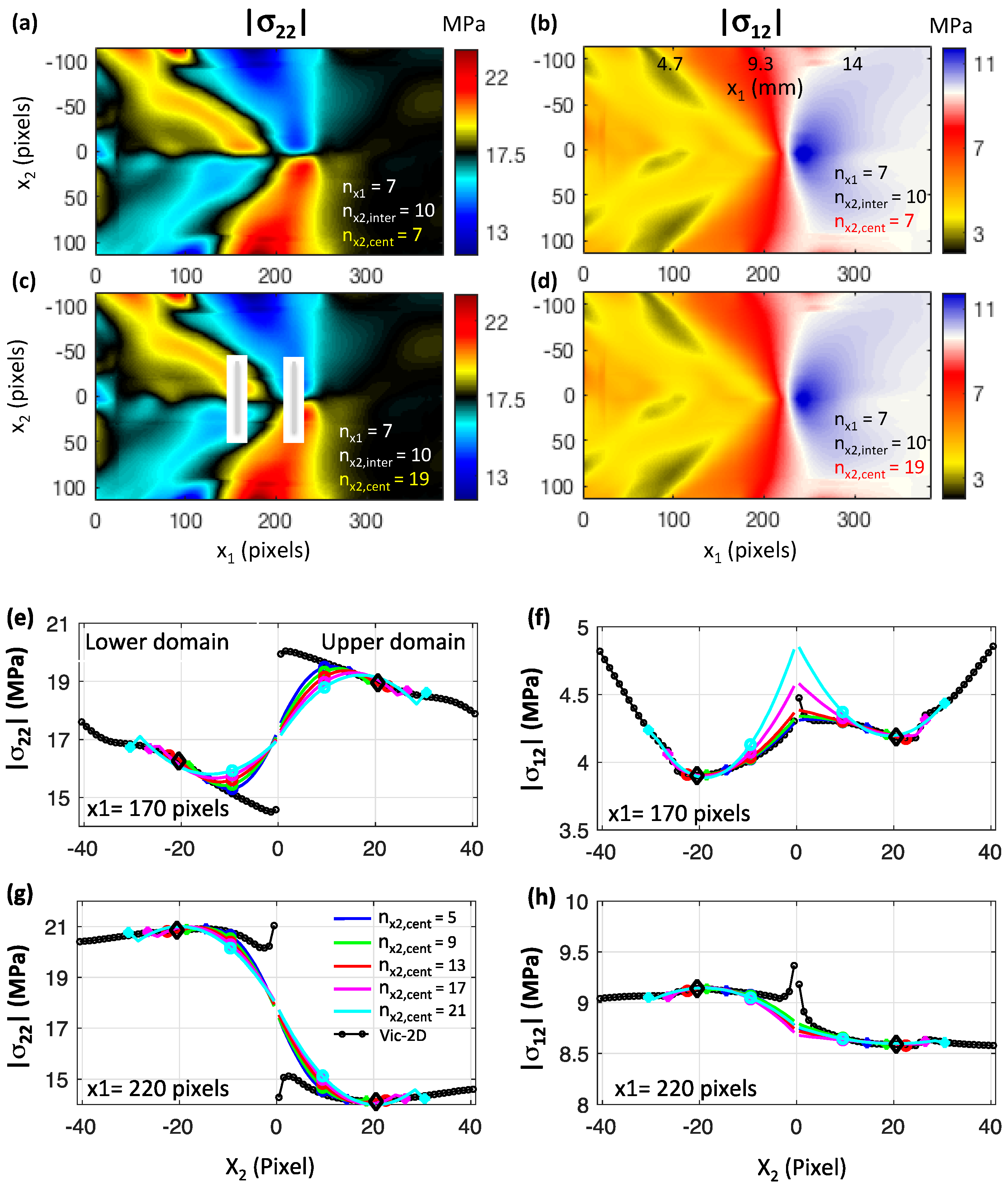
The effect of n_x2,cent was generally smaller than that of n_x2,inter. Full-field maps of stresses obtained with n_x2,cent = 7 and n_x2,inter = 10 (Figure 7a,b), were similar to those in Figure 2c,d. However, large value of n_x2,cent = 19 resulted in small discontinuities in normal stress at the pixels located n_x2 pixels above and below the interface (Figure 7c,d). Both at x₁ = 170 and 220 pixels there was a very small effect of n_x2,cent on the normal stress at the interface (Figure 7e,g). However, for n_x2,cent ≥ 17, the fit between the stresses obtained by the polynomial and the original stresses was poor also for the pixels closer to the center of the subset. Similarly to n_x2,inter, the shear stress at the interface may significantly have differed for large values of n_x2,cent (Figure 7f).

4. Implications for Friction Analysis

The experimental setup developed in [1,3], which combines ultra-high-speed photography with digital image correlation, enables us to observe displacements, velocities, and stresses close to the interface. For the field of view shown in Figure 1, these quantities can be measured up to 25 μm (0.5 pixels) from the interface using the “fill boundary” algorithm of Vic-2D. This enables studying the evolution of friction, defined by the ratio $f={\sigma }_{12}{}^0/{\sigma }_{22}{}^0$, at any point along the interface, as well as its dependence on variables such as slip (relative displacement across the interface) and slip rate [1]. As a first approach to enforce traction continuity on the interface, the tractions ${\sigma }_{12}{}^0$ and ${\sigma }_{22}{}^0$ were calculated in [1] by averaging the stresses at the pixels immediately above and below the interface. Because of the anti-symmetric and symmetric patterns in the stress changes $\Delta {\sigma }_{22}$ and $\Delta {\sigma }_{12}$, respectively, the normal stress on the interface ${\sigma }_{22}{}^0$ was inferred to be nearly constant, as expected during the propagation of a dynamic shear rupture along a planar interface, and the shear stress ${\sigma }_{12}{}^0$ had a smoother evolution than the individual components ${\sigma }_{12}^{0^{+}}$ and ${\sigma }_{12}^{0^{-}}$ above and below the interface. The averaging enabled us to study friction, despite large differences between the normal stresses immediately above and below the interface [1], but it is important to examine whether those average values actually correspond to the tractions at the interface computed with the continuity condition.

In general, the averaged normal stresses (without TC enforcement) agreed with the normal stresses computed with TC enforcement for the pixels immediately above and below the interface (Figure 8a), with some small deviations. Note that, because we enforced the continuity at the interface, the stresses obtained with TC enforcement for the pixels located 0.5 pixels above and below the interface did not completely overlap, with a maximum difference of 0.3 MPa. Because of its symmetry with respect to the interface, the discontinuity in shear stress across the interface for the original Vic-2d results (Figure 8b) was significantly smaller than in the normal stress. Overall, there was a good agreement between the shear tractions obtained by the averaging procedure and those obtained with TC enforcement, again, with some minor differences. Interestingly, the differences were consistently smaller in the cohesive zone (the zone where the shear traction drops from a maximum to a residual value), with a maximum difference of about 1 MPa at x₁ = 9 mm. This is also shown locally in Figure 5h. Because the stresses were computed from displacement gradients, small changes in the displacements were enough to enforce the traction continuity on the interface, and there were only minor differences between the interface-parallel displacements and velocities obtained with TC enforcement and those obtained without TC enforcement (Figure 8c,d). The small differences in stresses resulted in some differences in the evolution of local friction with slip and slip rate (Figure 8e,f). However, the important characteristics of the local friction, such as the peak, residual levels, and weakening distance, were similar.

5. Conclusions

In this work, the local DIC solution is supplemented with a fast post-processing algorithm to enforce the continuity of tractions across the interfaces of shear ruptures. This procedure allows us to obtain more physically meaningful stress fields near the interface, which is important when DIC is applied to study the dynamics of laboratory frictional ruptures. In the algorithm, the stresses near the interface are calculated from local polynomials that are constructed using a constrained inversion. This inversion is such that the resulting displacements match the displacements of pixels closer to the center of the subset, where the DIC solution is most accurate, while the resulting stresses satisfy traction continuity conditions at the interface.

We applied the algorithm to the displacement fields of a laboratory shear rupture obtained with a local DIC procedure, to show that the algorithm indeed produces the desired continuous traction fields across the interface. A sensitivity study provided a constraint on the parameters n_x2,inter, n_x2,cent, and n_x1 involved in the construction of the polynomials, such that undesired artifacts in the stress fields were eliminated. We found that parameter ranges of 8 ≤ n_x2,inter ≤ 14 (1/5 to 1/3 of the subset size) and 7 ≤ n_x2,cent ≤ 15 gave similar results, independent of the value of n_x1. Relatively minor changes in displacement fields around the interface can produce non-negligible gradient changes, resulting in some non-uniqueness regarding the exact stress evolution towards the interface, even if the traction continuity is enforced. Future progress can be made by combining the results inferred by the analysis presented in this work with dynamic rupture modeling that matches the observed full fields. The dynamic solutions can then be interrogated for the spatial dependencies of stress fields next to the interface.

The averaging procedure for stresses above and below the interface, employed in the previous study [1] to study friction, works well to mimic the traction continuity across the interface due to the special nature of this rupture problem that exhibits certain symmetries across the interface. However, the averaging procedure may not work as well in cases where the symmetries are disrupted, as in the case of ruptures approaching a free surface [27]. We will examine such cases in future studies.

References

- Rubino, V.; Rosakis, A.J.; Lapusta, N. Understanding dynamic friction through spontaneously evolving laboratory earthquakes. Nat. Commun. 2017, 8, 15991. [Google Scholar] [CrossRef] [PubMed]
- Gori, M.; Rubino, V.; Rosakis, A.J.; Lapusta, N. Pressure shock fronts formed by ultra-fast shear cracks in viscoelastic materials. Nat. Commun. 2018, 9, 4754. [Google Scholar]
- Rubino, V.; Rosakis, A.J.; Lapusta, N. Full-field ultrahigh-speed quantification of dynamic shear ruptures using digital image correlation. Exp. Mech. 2019, in press. [Google Scholar] [CrossRef]
- Sutton, M.A.; Orteu, J.J.; Schreier, H. Image Correlation for Shape, Motion and Deformation Measurements: Basic Concepts, Theory and Applications; Springer: New York, NY, USA, 2009. [Google Scholar]
- Hild, F.; Roux, S. Digital Image Correlation; Wiley-VCH: Weinheim, UK, 2012. [Google Scholar]
- Sutton, M.A.; Matta, F.; Rizos, D.; Ghorbani, R.; Rajan, S.; Mollenhauer, D.H.; Schreier, H.W.; Lasprilla, A.O. Recent Progress in Digital Image Correlation: Background and Developments since the 2013 W M Murray Lecture. Exp. Mech. 2017, 57, 1–30. [Google Scholar] [CrossRef]
- Hild, F.; Roux, S. Comparison of Local and Global Approaches to Digital Image Correlation. Exp. Mech. 2012, 52, 1503–1519. [Google Scholar] [CrossRef]
- Wang, B.; Pan, B. Subset-based local vs. finite element-based global digital image correlation: A comparison study. Theor. Appl. Mech. Lett. 2016, 6, 200–208. [Google Scholar] [CrossRef]
- Besnard, G.; Hild, F.; Roux, S. “Finite-element” displacement fields analysis from digital images: Application to Portevin-Le Châtelier bands. Exp. Mech. 2006, 46, 789–803. [Google Scholar] [CrossRef]
- Sun, Y.; Pang, J.H.; Wong, C.K.; Su, F. Finite element formulation for a digital image correlation method. Appl. Opt. 2005, 44, 7357–7363. [Google Scholar] [CrossRef]
- Sutton, M.A.; Wolters, W.J.; Peters, W.H.; Ranson, W.F.; McNeill, S.R. Determination of displacements using an improved digital correlation method. Image Vis. Comput. 1983, 1, 133–139. [Google Scholar] [CrossRef]
- Sutton, M.A.; Cheng, M.; Peters, W.H.; Chao, Y.J.; McNeill, S.R. Application of an optimized digital correlation method to planar deformation analysis. Image Vis. Comput. 1986, 4, 143–150. [Google Scholar] [CrossRef]
- Reu, P.L.; Toussaint, E.; Jones, E.; Bruck, H.A.; Iadicola, M.; Balcaen, R.; Turner, D.Z.; Siebert, T.; Lava, P.; Simonsen, M. DIC Challenge: Developing Images and Guidelines for Evaluating Accuracy and Resolution of 2D Analyses. Exp. Mech. 2018, 58, 1067–1099. [Google Scholar] [CrossRef]
- Rossi, M.; Lava, P.; Pierron, F.; Debruyne, D.; Sasso, M. Effect of DIC spatial resolution, noise and interpolation error on identification results with the VFM. Strain 2015, 51, 206–222. [Google Scholar] [CrossRef]
- Jin, H.; Bruck, H.A. Theoretical development for pointwise digital image correlation. Opt. Eng. 2005, 44, 067003. [Google Scholar] [CrossRef]
- Réthoré, J.; Hild, F.; Roux, S. Shear-band capturing using a multiscale extended digital image correlation technique. Comput. Methods Appl. Mech. Eng. 2007, 196, 5016–5030. [Google Scholar] [CrossRef]
- Réthoré, J.; Hild, F.; Roux, S. Extended digital image correlation with crack shape optimization. Int. J. Numer. Methods Eng. 2008, 73, 248–272. [Google Scholar] [CrossRef]
- Poissant, J.; Barthelat, F. A novel “subset splitting” procedure for digital image correlation on discontinuous displacement fields. Exp. Mech. 2010, 50, 353–364. [Google Scholar] [CrossRef]
- Nguyen, T.L.; Hall, S.A.; Vacher, P.; Viggiani, G. Fracture mechanisms in soft rock: Identification and quantification of evolving displacement discontinuities by extended digital image correlation. Tectonophysics 2011, 503, 117–128. [Google Scholar] [CrossRef]
- Tomicevic, Z.; Hild, F.; Roux, S.; Tomicevic, Z.; Hild, F.; Roux, S.; Image, M.D. Mechanics-Aided Digital Image Correlation. J. Strain Anal. Eng. Des. 2013, 48, 330–343. [Google Scholar] [CrossRef]
- Hassan, G.M.; Dyskin, A.; Macnish, C.; Pasternak, E.; Shufrin, I. Discontinuous Digital Image Correlation to reconstruct displacement and strain fields with discontinuities: Dislocation approach. Eng. Fract. Mech. 2018, 189, 273–292. [Google Scholar] [CrossRef]
- Hassan, G.M.; Macnish, C.; Dyskin, A. Extending Digital Image Correlation to Reconstruct Displacement and Strain Fields around Discontinuities in Geomechanical Structures under Deformation. In Proceedings of the IEEE Winter Conference on Applications of Computer Vision, Waikoloa, HI, USA, 5–9 January 2015; IEEE: Piscataway, NJ, USA, 2015; pp. 710–717. [Google Scholar]
- Rubino, V.; Lapusta, N.; Rosakis, A.J.; Leprince, S.; Avouac, J.P. Static Laboratory Earthquake Measurements with the Digital Image Correlation Method. Exp. Mech. 2015, 55, 77–94. [Google Scholar] [CrossRef]
- Xia, K.; Rosakis, A.J.; Kanamori, H. Laboratory Earthquakes: The Sub-Rayleigh-to-Supershear. Science 2004, 303, 1859–1861. [Google Scholar] [CrossRef]
- Lu, X.; Lapusta, N.; Rosakis, A.J. Pulse-like and crack-like ruptures in experiments mimicking crustal earthquakes. Proc. Natl. Acad. Sci. USA 2007, 104, 18931–18936. [Google Scholar] [CrossRef] [PubMed]
- Rosakis, A.J.; Xia, K.; Lykotrafitis, G.; Kanamori, H. Dynamic shear rupture in frictional interfaces: Speeds, directionality, and modes. Treatise Geophys. 2007, 4, 153–192. [Google Scholar]
- Gabuchian, V.; Rosakis, A.J.; Bhat, H.S.; Madariaga, R.; Kanamori, H. Experimental evidence that thrust earthquake ruptures might open faults. Nature 2017, 545, 336–339. [Google Scholar] [CrossRef]
- Mello, M.; Bhat, H.S.; Rosakis, A.J.; Kanamori, H. Identifying the unique ground motion signatures of supershear earthquakes: Theory and experiments. Tectonophysics 2010, 493, 297–326. [Google Scholar] [CrossRef]
- Mello, M.; Bhat, H.S.; Rosakis, A.J.; Kanamori, H. Reproducing the supershear portion of the 2002 Denali earthquake rupture in laboratory. Earth Planet. Sci. Lett. 2014, 387, 89–96. [Google Scholar] [CrossRef]
- Buades, A.; Coll, B.; Morel, J. The Staircasing Effect in Neighborhood Filters and its Solution. IEEE Trans. Image Process. 2006, 15, 1499–1505. [Google Scholar] [CrossRef] [PubMed]
- Buades, A.; Coll, B.; Morel, J. Nonlocal Image and Movie Denoising. Int. J. Comput. Vis. 2008, 76, 123–139. [Google Scholar] [CrossRef]
- Rosakis, A.; Samudrala, O.; Coker, D. Cracks faster than the shear wave speed. Science 1999, 284, 1337–1340. [Google Scholar] [CrossRef] [PubMed]
- Rosakis, A.J. Intersonic shear cracks and fault ruptures. Adv. Phys. 2002, 51, 1189–1257. [Google Scholar] [CrossRef]
Figure 1.
Schematics of the laboratory rupture experiment. Dynamic shear ruptures evolved spontaneously along the frictional interface, inclined at an angle α, of two Homalite plates under a compressional load P. Ruptures were initiated by the small burst of a NiCr wire placed across the interface and connected to a capacitor bank. The white light produced by a flash source was reflected by the specimen’s surface and captured by a low-noise high-speed camera, typically at 1–2 million frames/s. The portion of the specimen to be imaged, the field of view, was coated by a flat white paint and decorated by a characteristic speckle pattern. Next, the textured images were processed by digital image correlation (DIC) algorithms to produce a temporal sequence of full-field displacement maps. The displacement fields were then post-processed to produce velocity, strain, strain rate, and stress maps.
Figure 2.
Full-field maps of normal (left) and shear (right) stresses measured for a super-shear crack-like rupture during a test with α = 29°, P = 23 MPa ( MPa and MPa), and a field of view of 19 x 12 mm. (a,b) Full-field maps obtained using Vic-2D extrapolation near the interface. (c,d) Fulfilled maps obtained with the stress continuity constraints, using a good set of parameters nx1, nx2,inter, and nx2,cent. (e–h) Enforcement of stress continuity with extreme values of nx2,inter and nx2,cent leads to discontinuities and spurious oscillations in the stress fields. Note that the full-field maps are cropped and their size is slightly smaller than the reported field of view size.
Figure 3.
(a) A speckled image with two subsets of 41 × 41 pixels above and below the interface (yellow squares). The post-processing algorithm is performed on the regions inside the subsets marked by the red rectangles. (b) The geometry of the pixels over which the local polynomials approximating the displacement fields are defined. The polynomials approximating , extend over a rectangle above the interface, while those approximating , extend over a rectangle below the interface; both rectangles include pixels. The pixels within each rectangle are divided into a group of pixels that are closer to the interface, and a group of pixels that are closer to the center of the subset. The observed displacements in the latter group are used together with continuity of stresses constraints on the interface to construct the polynomials. (c,d) Two different combinations of and and their relationship with Vic-2D extrapolation. In the first combination, the group of pixels , which are used as data in the inversion, include pixels where the displacement values were obtained by the “fill boundary” algorithm of Vic-2D.
Figure 4.
Interface parallel (a) and normal (b) displacements at the central columns of the subsets shown in Figure 3a. The black lines represent the displacements obtained with Vic-2D, while the blue lines are the displacements modified with the traction continuity algorithm, using , , and . The red circles represent the observed displacements that are used to invert for the coefficients of the displacement polynomials , , , and . The black diamonds correspond to the centers of the subsets.
Figure 5.
The effect of parameter nx1 on the stress field. (a–d) Full-field maps of normal (left) and shear (right) stresses for nx1 = 3 and 9. (e–h) Normal (left) and shear (right) stresses vs position along paths perpendicular to the interface at x1 = 170 and 220 pixels (grey lines in (c)) for different values of nx1. The stresses calculated with the “fill boundary” algorithm of Vic-2D without the traction continuity algorithm are also shown, where the black diamonds correspond to the centers of the subsets above and below the interface. In all the cases shown in this figure, nx2,inter = 10 and nx2,cent = 11.
Figure 6.
The effect of parameter nx2,inter on the stress field. (a–d) Full-field maps of normal (left) and shear (right) stresses for nx2,inter = 6 and 16. (e–h) Normal (left) and shear (right) stresses vs position along paths perpendicular to the interface at x1 = 170 and 220 pixels (grey lines in (c)) for different values of nx2,inter. The circles on the curves correspond to nx2,inter, while the filled diamonds correspond to nx2. The stresses calculated with the “fill boundary” algorithm of Vic-2D without the traction continuity algorithm are also shown, where the black diamonds correspond to the centers of the subsets above and below the interface. In all the cases shown in this figure nx1 = 7 and nx2,cent = 11.
Figure 7.
The effect of parameter nx2,cent on the stress field. (a–d) Full-field maps of normal (left) and shear (right) stresses for nx2,cent = 7 and 19. (e–h) Normal (left) and shear (right) stresses vs position along paths perpendicular to the interface at x1 = 170 and 220 pixels (grey lines in (c)) for different values of nx2,cent. The circles on the curves correspond to nx2,inter, while the filled diamonds correspond to nx2. The stresses calculated with the “fill boundary” algorithm of Vic-2D without the traction continuity algorithm are also shown, where the black diamonds correspond to the centers of the subsets above and below the interface. In all the cases shown in this figure nx1 = 7 and nx2,inter = 10.
Figure 8.
(a,b) normal and shear stresses along the interface. The black curves represent the stresses ±0.5 pixels from the interface obtained without traction continuity (TC) enforcement, while the green curve represents the average of the two. The blue curves represent the stresses obtained with TC enforcement ±0.5 pixels from the interface. (c,d) Interface-parallel displacements and velocities ±0.5 pixels from the interface, obtained with (blue) and without (black) TC enforcement. (e,f) Resolved friction vs slip and slip rate at x1 = 8.5 mm, obtained with (blue) and without (black) TC enforcement. Both curves represent the average of the values immediately above and below interface. The polynomial geometrical parameters are nx1 = 7, nx2,inter = 10, and nx2,cent = 11.
© 2019 by the authors. Licensee MDPI, Basel, Switzerland. This article is an open access article distributed under the terms and conditions of the Creative Commons Attribution (CC BY) license (http://creativecommons.org/licenses/by/4.0/).
Share and Cite
MDPI and ACS Style
Tal, Y.; Rubino, V.; Rosakis, A.J.; Lapusta, N. Enhanced Digital Image Correlation Analysis of Ruptures with Enforced Traction Continuity Conditions Across Interfaces. Appl. Sci. 2019, 9, 1625. https://doi.org/10.3390/app9081625
AMA Style
Tal Y, Rubino V, Rosakis AJ, Lapusta N. Enhanced Digital Image Correlation Analysis of Ruptures with Enforced Traction Continuity Conditions Across Interfaces. Applied Sciences. 2019; 9(8):1625. https://doi.org/10.3390/app9081625
Chicago/Turabian StyleTal, Yuval, Vito Rubino, Ares J. Rosakis, and Nadia Lapusta. 2019. "Enhanced Digital Image Correlation Analysis of Ruptures with Enforced Traction Continuity Conditions Across Interfaces" Applied Sciences 9, no. 8: 1625. https://doi.org/10.3390/app9081625
Note that from the first issue of 2016, this journal uses article numbers instead of page numbers. See further details here.