Independent Components of EEG Activity Correlating with Emotional State

 ,
,
Abstract
:1. Introduction
2. Materials and Methods
2.1. Participants
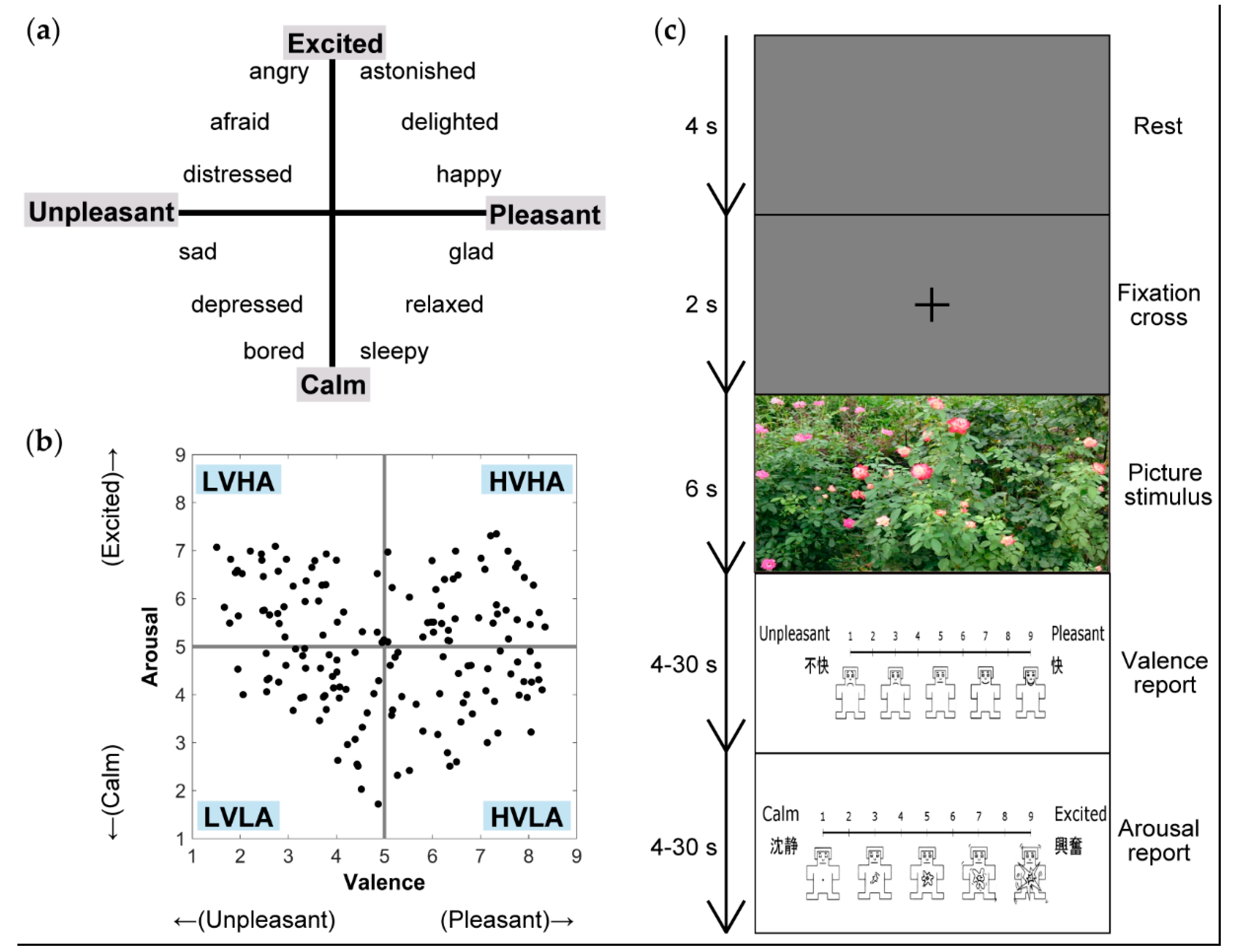
2.2. Stimuli
2.3. Experimental Task
2.4. EEG Data Acquisition
2.5. EEG Data Processing
2.6. Regression Analyses
2.7. Identification of IC Clusters Correlating with Emotional State
3. Results
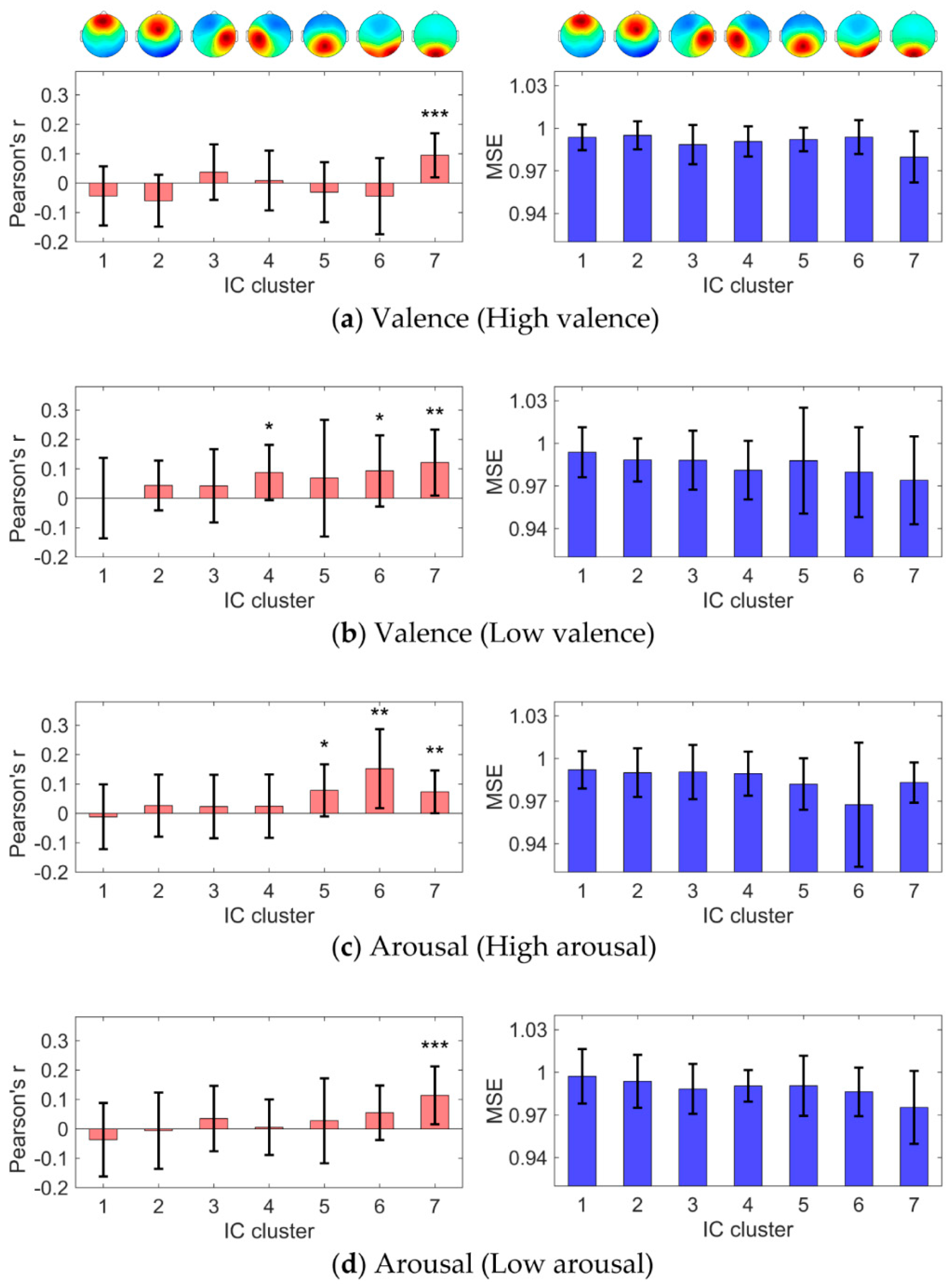
3.1. IC Clusters Obtained by ICA and Cluster Analysis
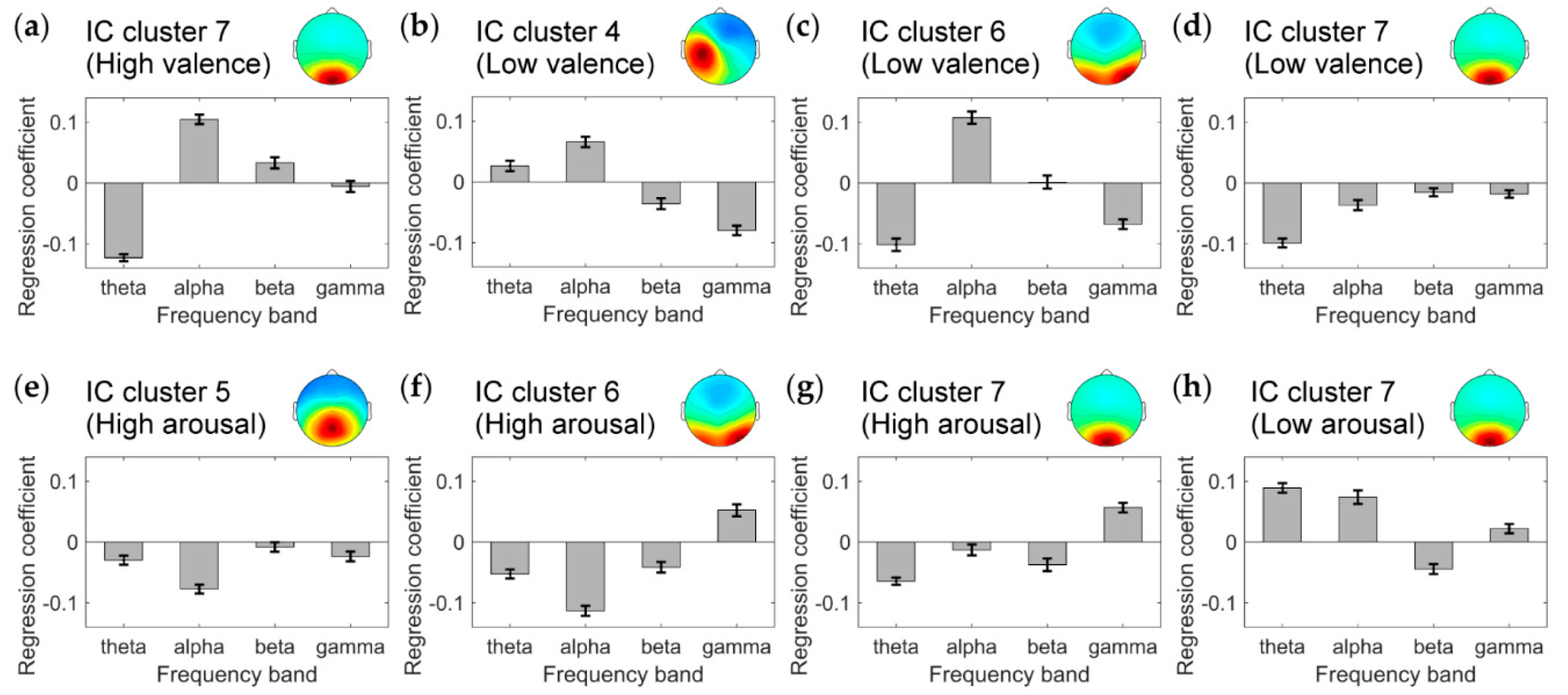
3.2. IC Clusters Correlating with Emotional State
4. Discussion
5. Conclusions
Author Contributions
Funding
Acknowledgments
Conflicts of Interest
References
- Kim, M.-K.; Kim, M.; Oh, E.; Kim, S.-P. A Review on the Computational Methods for Emotional State Estimation from the Human EEG. Comput. Math. Methods Med. 2013, 2013, 573734. [Google Scholar] [CrossRef] [PubMed] [Green Version]
- Al-Nafjan, A.; Hosny, M.; Al-Ohali, Y.; Al-Wabil, A. Review and Classification of Emotion Recognition Based on EEG Brain-Computer Interface System Research: A Systematic Review. Appl. Sci. 2017, 7, 1239. [Google Scholar] [CrossRef] [Green Version]
- Alarcão, S.M.; Fonseca, M.J. Emotions Recognition Using EEG Signals: A Survey. IEEE Trans. Affect. Comput. 2019, 10, 374–393. [Google Scholar] [CrossRef]
- Frantzidis, C.A.; Bratsas, C.; Papadelis, C.L.; Konstantinidis, E.; Pappas, C.; Bamidis, P.D. Toward Emotion Aware Computing: An Integrated Approach Using Multichannel Neurophysiological Recordings and Affective Visual Stimuli. IEEE Trans. Inf. Technol. Biomed. 2010, 14, 589–597. [Google Scholar] [CrossRef] [PubMed]
- Russell, J.A. A circumplex model of affect. J. Personal. Soc. Psychol. 1980, 39, 1161–1178. [Google Scholar] [CrossRef]
- Padilla-Buritica, J.I.; Martinez-Vargas, J.D.; Castellanos-Dominguez, G. Emotion Discrimination Using Spatially Compact Regions of Interest Extracted from Imaging EEG Activity. Front. Comput. Neurosci. 2016, 10, 55. [Google Scholar] [CrossRef] [PubMed] [Green Version]
- Martinez-Vargas, J.D.; Nieto-Mora, D.A.; Muñoz-Gutiérrez, P.A.; Cespedes-Villar, Y.R.; Giraldo, E.; Castellanos-Dominguez, G. Assessment of Source Connectivity for Emotional States Discrimination. In Brain Informatics (BI 2018), Proceedings of the International Conference on Brain Informatics, Arlington, TX, USA, 7–9 December, 2018; Springer: Cham, Switzerland, 2018; pp. 63–73. [Google Scholar]
- Becker, H.; Fleureau, J.; Guillotel, P.; Wendling, F.; Merlet, I.; Albera, L. Emotion Recognition Based on High-Resolution EEG Recordings and Reconstructed Brain Sources. IEEE Trans. Affect. Comput. 2020, 11, 244–257. [Google Scholar] [CrossRef]
- Chen, G.; Zhang, X.; Sun, Y.; Zhang, J. Emotion Feature Analysis and Recognition Based on Reconstructed EEG Sources. IEEE Access 2020, 8, 11907–11916. [Google Scholar] [CrossRef]
- Hu, X.; Chen, J.; Wang, F.; Zhang, D. Ten challenges for EEG-based affective computing. Brain Sci. Adv. 2019, 5, 1–20. [Google Scholar] [CrossRef] [Green Version]
- Bradley, M.M.; Lang, P.J. Measuring emotion: The self-assessment manikin and the semantic differential. J. Behav. Ther. Exp. Psychiatry 1994, 25, 49–59. [Google Scholar] [CrossRef]
- Soleymani, M.; Koelstra, S.; Patras, I.; Pun, T. Continuous emotion detection in response to music videos. In Proceedings of the Face and Gesture 2011, Santa Barbara, CA, USA, 21–25 March 2011; pp. 803–808. [Google Scholar]
- Uzun, S.S.; Yildirim, S.; Yildirim, E. Emotion primitives estimation from EEG signals using Hilbert Huang Transform. In Proceedings of the 2012 IEEE-EMBS International Conference on Biomedical and Health Informatics, Hong Kong, China, 5–7 January 2012; pp. 224–227. [Google Scholar]
- Garcia, H.F.; Orozco, Á.A.; Álvarez, M.A. Dynamic physiological signal analysis based on Fisher kernels for emotion recognition. In Proceedings of the 2013 35th Annual International Conference of the IEEE Engineering in Medicine and Biology Society (EMBC), Osaka, Japan, 3–7 July 2013; pp. 4322–4325. [Google Scholar]
- Jenke, R.; Peer, A.; Buss, M. A Comparison of Evaluation Measures for Emotion Recognition in Dimensional Space. In Proceedings of the 2013 Humaine Association Conference on Affective Computing and Intelligent Interaction, Geneva, Switzerland, 2–5 September 2013; pp. 822–826. [Google Scholar]
- Koelstra, S.; Patras, I. Fusion of facial expressions and EEG for implicit affective tagging. Image Vis. Comput. 2013, 31, 164–174. [Google Scholar] [CrossRef]
- Soleymani, M.; Asghari-Esfeden, S.; Pantic, M.; Fu, Y. Continuous emotion detection using EEG signals and facial expressions. In Proceedings of the 2014 IEEE International Conference on Multimedia and Expo (ICME), Chengdu, China, 14–18 July 2014; pp. 1–6. [Google Scholar]
- Torres-Valencia, C.A.; Álvarez, M.A.; Orozco-Gutiérrez, Á.A. Multiple-output support vector machine regression with feature selection for arousal/valence space emotion assessment. In Proceedings of the 2014 36th Annual International Conference of the IEEE Engineering in Medicine and Biology Society, Chicago, IL, USA, 26–30 August 2014; pp. 970–973. [Google Scholar]
- Zhuang, X.; Rozgić, V.; Crystal, M. Compact unsupervised EEG response representation for emotion recognition. In Proceedings of the IEEE-EMBS International Conference on Biomedical and Health Informatics (BHI), Valencia, Spain, 1–4 June 2014; pp. 736–739. [Google Scholar]
- Al-Fahad, R.; Yeasin, M. Robust Modeling of Continuous 4-D Affective Space from EEG Recording. In Proceedings of the 2016 15th IEEE International Conference on Machine Learning and Applications (ICMLA), Anaheim, CA, USA, 18–20 December 2016; pp. 1040–1045. [Google Scholar]
- Lan, Z.; Müller-Putz, G.R.; Wang, L.; Liu, Y.; Sourina, O.; Scherer, R. Using Support Vector Regression to estimate valence level from EEG. In Proceedings of the 2016 IEEE International Conference on Systems, Man, and Cybernetics (SMC), Budapest, Hungary, 9–12 October 2016; pp. 2558–2563. [Google Scholar]
- McFarland, D.J.; Parvaz, M.A.; Sarnacki, W.A.; Goldstein, R.Z.; Wolpaw, J.R. Prediction of subjective ratings of emotional pictures by EEG features. J. Neural Eng. 2016, 14, 016009. [Google Scholar] [CrossRef] [PubMed]
- Soleymani, M.; Asghari-Esfeden, S.; Fu, Y.; Pantic, M. Analysis of EEG Signals and Facial Expressions for Continuous Emotion Detection. IEEE Trans. Affect. Comput. 2016, 7, 17–28. [Google Scholar] [CrossRef]
- Thammasan, N.; Fukui, K.; Numao, M. An investigation of annotation smoothing for EEG-based continuous music-emotion recognition. In Proceedings of the 2016 IEEE International Conference on Systems, Man, and Cybernetics (SMC), Budapest, Hungary, 9–12 October 2016; pp. 3323–3328. [Google Scholar]
- Al-Fahad, R.; Yeasin, M.; Anam, A.S.M.I.; Elahian, B. Selection of stable features for modeling 4-D affective space from EEG recording. In Proceedings of the 2017 International Joint Conference on Neural Networks (IJCNN), Anchorage, AK, USA, 14–19 May 2017; pp. 1202–1209. [Google Scholar]
- Thammasan, N.; Fukui, K.; Numao, M. Application of Annotation Smoothing for Subject-Independent Emotion Recognition Based on Electroencephalogram. In Trends in Artificial Intelligence: PRICAI 2016 Workshops, Proceedings of the Pacific Rim International Conference on Artificial Intelligence, Phuket, Thailand, 22–23 August 2016; Springer: Cham, Switzerland, 2017; pp. 115–126. [Google Scholar]
- Ding, Y.; Hu, X.; Xia, Z.; Liu, Y.; Zhang, D. Inter-brain EEG Feature Extraction and Analysis for Continuous Implicit Emotion Tagging during Video Watching. IEEE Trans. Affect. Comput. 2018. [Google Scholar] [CrossRef]
- Reali, P.; Cosentini, C.; de Carvalho, P.; Traver, V.; Bianchi, A.M. Towards the development of physiological models for emotions evaluation. In Proceedings of the 2018 40th Annual International Conference of the IEEE Engineering in Medicine and Biology Society (EMBC), Honolulu, HI, USA, 18–21 July 2018; pp. 110–113. [Google Scholar]
- Sani, O.G.; Yang, Y.; Lee, M.B.; Dawes, H.E.; Chang, E.F.; Shanechi, M.M. Mood variations decoded from multi-site intracranial human brain activity. Nat. Biotechnol. 2018, 36, 954–961. [Google Scholar] [CrossRef]
- Yao, Y.; Qing, C.; Xu, X.; Wang, Y. EEG-Based Emotion Estimate Using Shallow Fully Convolutional Neural Network with Boost Training Strategy. In Advances in Brain Inspired Cognitive Systems, Proceedings of the International Conference on Brain Inspired Cognitive Systems, Guangzhou, China, 13–14 July 2019; Springer: Cham, Switzerland, 2020; pp. 55–64. [Google Scholar]
- Onton, J.; Makeig, S. Information-based modeling of event-related brain dynamics. Prog. Brain Res. 2006, 159, 99–120. [Google Scholar] [CrossRef] [Green Version]
- Liu, J.; Tian, J. Spatiotemporal analysis of single-trial EEG of emotional pictures based on independent component analysis and source location. In Medical Imaging 2007: Physiology, Function, and Structure from Medical Images; SPIE: Washington, DC, USA, 2007; Volume 6511, pp. 646–655. [Google Scholar]
- Onton, J.; Makeig, S. High-frequency broadband modulations of electroencephalographic spectra. Front. Hum. Neurosci. 2009, 3, 61. [Google Scholar] [CrossRef] [Green Version]
- Lin, Y.-P.; Duann, J.-R.; Chen, J.-H.; Jung, T.-P. Electroencephalographic dynamics of musical emotion perception revealed by independent spectral components. Neuroreport 2010, 21, 410–415. [Google Scholar] [CrossRef]
- Wyczesany, M.; Ligeza, T.S. Towards a constructionist approach to emotions: Verification of the three-dimensional model of affect with EEG-independent component analysis. Exp. Brain Res. 2015, 233, 723–733. [Google Scholar] [CrossRef] [Green Version]
- Rogenmoser, L.; Zollinger, N.; Elmer, S.; Jäncke, L. Independent component processes underlying emotions during natural music listening. Soc. Cogn. Affect. Neurosci. 2016, 11, 1428–1439. [Google Scholar] [CrossRef] [Green Version]
- Shen, Y.-W.; Lin, Y.-P. Challenge for Affective Brain-Computer Interfaces: Non-stationary Spatio-spectral EEG Oscillations of Emotional Responses. Front. Hum. Neurosci. 2019, 13, 366. [Google Scholar] [CrossRef] [PubMed]
- Machizawa, M.G.; Lisi, G.; Kanayama, N.; Mizuochi, R.; Makita, K.; Sasaoka, T.; Yamawaki, S. Quantification of anticipation of excitement with a three-axial model of emotion with EEG. J. Neural Eng. 2020, 17, 036011. [Google Scholar] [CrossRef] [PubMed]
- Nielen, M.M.A.; Heslenfeld, D.J.; Heinen, K.; Van Strien, J.W.; Witter, M.P.; Jonker, C.; Veltman, D.J. Distinct brain systems underlie the processing of valence and arousal of affective pictures. Brain Cogn. 2009, 71, 387–396. [Google Scholar] [CrossRef] [PubMed]
- Viinikainen, M.; Jääskeläinen, I.P.; Alexandrov, Y.; Balk, M.H.; Autti, T.; Sams, M. Nonlinear relationship between emotional valence and brain activity: Evidence of separate negative and positive valence dimensions. Hum. Brain Mapp. 2010, 31, 1030–1040. [Google Scholar] [CrossRef] [PubMed]
- Lang, P.J.; Bradley, M.M.; Cuthbert, B.N. International Affective Picture System (IAPS): Affective Ratings of Pictures and Instruction Manual; Technical Report A-8; University of Florida: Gainesville, FL, USA, 2008. [Google Scholar]
- Brainard, D.H. The Psychophysics Toolbox. Spat. Vis. 1997, 10, 433–436. [Google Scholar] [CrossRef] [PubMed] [Green Version]
- Pelli, D.G. The VideoToolbox software for visual psychophysics: Transforming numbers into movies. Spat. Vis. 1997, 10, 437–442. [Google Scholar] [CrossRef] [Green Version]
- Kleiner, M.; Brainard, D.; Pelli, D. What’s new in Psychtoolbox-3? Perception 2007, 36. [Google Scholar]
- Delorme, A.; Makeig, S. EEGLAB: An open source toolbox for analysis of single-trial EEG dynamics including independent component analysis. J. Neurosci. Methods 2004, 134, 9–21. [Google Scholar] [CrossRef] [Green Version]
- Palmer, J.A.; Makeig, S.; Kreutz-Delgado, K.; Rao, B.D. Newton method for the ICA mixture model. In Proceedings of the 2008 IEEE International Conference on Acoustics, Speech and Signal Processing, Lag Vegas, NV, USA, 31 March–4 April 2008; pp. 1805–1808. [Google Scholar]
- Oostenveld, R.; Fries, P.; Maris, E.; Schoffelen, J.-M. FieldTrip: Open Source Software for Advanced Analysis of MEG, EEG, and Invasive Electrophysiological Data. Comput. Intell. Neurosci. 2011, 2011, 156869. [Google Scholar] [CrossRef]
- Tzourio-Mazoyer, N.; Landeau, B.; Papathanassiou, D.; Crivello, F.; Etard, O.; Delcroix, N.; Mazoyer, B.; Joliot, M. Automated Anatomical Labeling of Activations in SPM Using a Macroscopic Anatomical Parcellation of the MNI MRI Single-Subject Brain. Neuroimage 2002, 15, 273–289. [Google Scholar] [CrossRef]
- Rorden, C.; Karnath, H.-O.; Bonilha, L. Improving Lesion-Symptom Mapping. J. Cogn. Neurosci. 2007, 19, 1081–1088. [Google Scholar] [CrossRef] [PubMed]
- Holm, S. A Simple Sequentially Rejective Multiple Test Procedure. Scand. J. Stat. 1979, 6, 65–70. [Google Scholar]
- Hamann, S.; Canli, T. Individual differences in emotion processing. Curr. Opin. Neurobiol. 2004, 14, 233–238. [Google Scholar] [CrossRef]
- Lang, P.J.; Bradley, M.M.; Fitzsimmons, J.R.; Cuthbert, B.N.; Scott, J.D.; Moulder, B.; Nangia, V. Emotional arousal and activation of the visual cortex: An fMRI analysis. Psychophysiology 1998, 35, 199–210. [Google Scholar] [CrossRef] [PubMed]
- Aftanas, L.I.; Varlamov, A.A.; Pavlov, S.V.; Makhnev, V.P.; Reva, N.V. Affective picture processing: Event-related synchronization within individually defined human theta band is modulated by valence dimension. Neurosci. Lett. 2001, 303, 115–118. [Google Scholar] [CrossRef]
- Güntekin, B.; Başar, E. A review of brain oscillations in perception of faces and emotional pictures. Neuropsychologia 2014, 58, 33–51. [Google Scholar] [CrossRef]
- Zhang, W.; Li, X.; Liu, X.; Duan, X.; Wang, D.; Shen, J. Distraction reduces theta synchronization in emotion regulation during adolescence. Neurosci. Lett. 2013, 550, 81–86. [Google Scholar] [CrossRef]
- Uusberg, A.; Thiruchselvam, R.; Gross, J.J. Using distraction to regulate emotion: Insights from EEG theta dynamics. Int. J. Psychophysiol. 2014, 91, 254–260. [Google Scholar] [CrossRef]
- Spyropoulos, G.; Bosman, C.A.; Fries, P. A theta rhythm in macaque visual cortex and its attentional modulation. Proc. Natl. Acad. Sci. USA 2018, 115, E5614–E5623. [Google Scholar] [CrossRef] [Green Version]
- Cavanna, A.E.; Trimble, M.R. The precuneus: A review of its functional anatomy and behavioural correlates. Brain 2006, 129, 564–583. [Google Scholar] [CrossRef] [Green Version]
- Cuthbert, B.N.; Schupp, H.T.; Bradley, M.M.; Birbaumer, N.; Lang, P.J. Brain potentials in affective picture processing: Covariation with autonomic arousal and affective report. Biol. Psychol. 2000, 52, 95–111. [Google Scholar] [CrossRef] [Green Version]
- Schupp, H.T.; Cuthbert, B.N.; Bradley, M.M.; Cacioppo, J.T.; Ito, T.; Lang, P.J. Affective picture processing: The late positive potential is modulated by motivational relevance. Psychophysiology 2000, 37, 257–261. [Google Scholar] [CrossRef] [PubMed]
- Olofsson, J.K.; Nordin, S.; Sequeira, H.; Polich, J. Affective picture processing: An integrative review of ERP findings. Biol. Psychol. 2008, 77, 247–265. [Google Scholar] [CrossRef] [PubMed] [Green Version]
- Hajcak, G.; MacNamara, A.; Olvet, D.M. Event-Related Potentials, Emotion, and Emotion Regulation: An Integrative Review. Dev. Neuropsychol. 2010, 35, 129–155. [Google Scholar] [CrossRef]
- Liu, Y.; Huang, H.; McGinnis-Deweese, M.; Keil, A.; Ding, M. Neural Substrate of the Late Positive Potential in Emotional Processing. J. Neurosci. 2012, 32, 14563–14572. [Google Scholar] [CrossRef] [Green Version]
- Cacioppo, J.T.; Berntson, G.G. Relationship between attitudes and evaluative space: A critical review, with emphasis on the separability of positive and negative substrates. Psychol. Bull. 1994, 115, 401–423. [Google Scholar] [CrossRef]
- Ekman, P. An argument for basic emotions. Cogn. Emot. 1992, 6, 169–200. [Google Scholar] [CrossRef]
- Pfurtscheller, G.; Aranibar, A. Evaluation of event-related desynchronization (ERD) preceding and following voluntary self-paced movement. Electroencephalogr. Clin. Neurophysiol. 1979, 46, 138–146. [Google Scholar] [CrossRef]
- Crone, N.E.; Miglioretti, D.L.; Gordon, B.; Lesser, R.P. Functional mapping of human sensorimotor cortex with electrocorticographic spectral analysis. II. Event-related synchronization in the gamma band. Brain 1998, 121, 2301–2315. [Google Scholar] [CrossRef] [Green Version]
- Leech, R.; Sharp, D.J. The role of the posterior cingulate cortex in cognition and disease. Brain 2014, 137, 12–32. [Google Scholar] [CrossRef] [Green Version]
- Foxe, J.J.; Snyder, A.C. The Role of Alpha-Band Brain Oscillations as a Sensory Suppression Mechanism during Selective Attention. Front. Psychol. 2011, 2, 154. [Google Scholar] [CrossRef] [PubMed] [Green Version]
- Phan, K.L.; Wager, T.; Taylor, S.F.; Liberzon, I. Functional Neuroanatomy of Emotion: A Meta-Analysis of Emotion Activation Studies in PET and fMRI. Neuroimage 2002, 16, 331–348. [Google Scholar] [CrossRef] [Green Version]
- Etkin, A.; Egner, T.; Kalisch, R. Emotional processing in anterior cingulate and medial prefrontal cortex. Trends Cogn. Sci. 2011, 15, 85–93. [Google Scholar] [CrossRef] [Green Version]
- Petrantonakis, P.C.; Hadjileontiadis, L.J. A Novel Emotion Elicitation Index Using Frontal Brain Asymmetry for Enhanced EEG-Based Emotion Recognition. IEEE Trans. Inf. Technol. Biomed. 2011, 15, 737–746. [Google Scholar] [CrossRef] [PubMed]
- Petrantonakis, P.C.; Hadjileontiadis, L.J. Adaptive Emotional Information Retrieval From EEG Signals in the Time-Frequency Domain. IEEE Trans. Signal Process. 2012, 60, 2604–2616. [Google Scholar] [CrossRef]


| Cluster Index | Location of Centroid 1 | MNI Coordinates (X, Y, Z) | Number of Participants | Number of ICs |
|---|---|---|---|---|
| 1 | Right anterior cingulate gyrus | (2, 39, −2) | 14 | 21 |
| 2 | Right middle cingulate gyrus | (1, −5, 32) | 14 | 21 |
| 3 | Right precentral gyrus | (39, −6, 36) | 16 | 18 |
| 4 | Left precentral gyrus | (−28, −13, 43) | 16 | 19 |
| 5 | Left middle cingulate gyrus | (−3, −40, 44) | 16 | 24 |
| 6 | Right precuneus | (20, −45, 4) | 18 | 19 |
| 7 | Right cuneus | (6, −84, 16) | 19 | 19 |
© 2020 by the authors. Licensee MDPI, Basel, Switzerland. This article is an open access article distributed under the terms and conditions of the Creative Commons Attribution (CC BY) license (http://creativecommons.org/licenses/by/4.0/).
Share and Cite
Maruyama, Y.; Ogata, Y.; Martínez-Tejada, L.A.; Koike, Y.; Yoshimura, N. Independent Components of EEG Activity Correlating with Emotional State. Brain Sci. 2020, 10, 669. https://doi.org/10.3390/brainsci10100669
Maruyama Y, Ogata Y, Martínez-Tejada LA, Koike Y, Yoshimura N. Independent Components of EEG Activity Correlating with Emotional State. Brain Sciences. 2020; 10(10):669. https://doi.org/10.3390/brainsci10100669
Chicago/Turabian StyleMaruyama, Yasuhisa, Yousuke Ogata, Laura A. Martínez-Tejada, Yasuharu Koike, and Natsue Yoshimura. 2020. "Independent Components of EEG Activity Correlating with Emotional State" Brain Sciences 10, no. 10: 669. https://doi.org/10.3390/brainsci10100669
APA StyleMaruyama, Y., Ogata, Y., Martínez-Tejada, L. A., Koike, Y., & Yoshimura, N. (2020). Independent Components of EEG Activity Correlating with Emotional State. Brain Sciences, 10(10), 669. https://doi.org/10.3390/brainsci10100669