
Effects of Phase Separation Behavior on Morphology and Performance of Polycarbonate Membranes


Abstract
:1. Introduction
2. Materials and Methods
2.1. Materials
2.2. Preparation of Polymer Solution
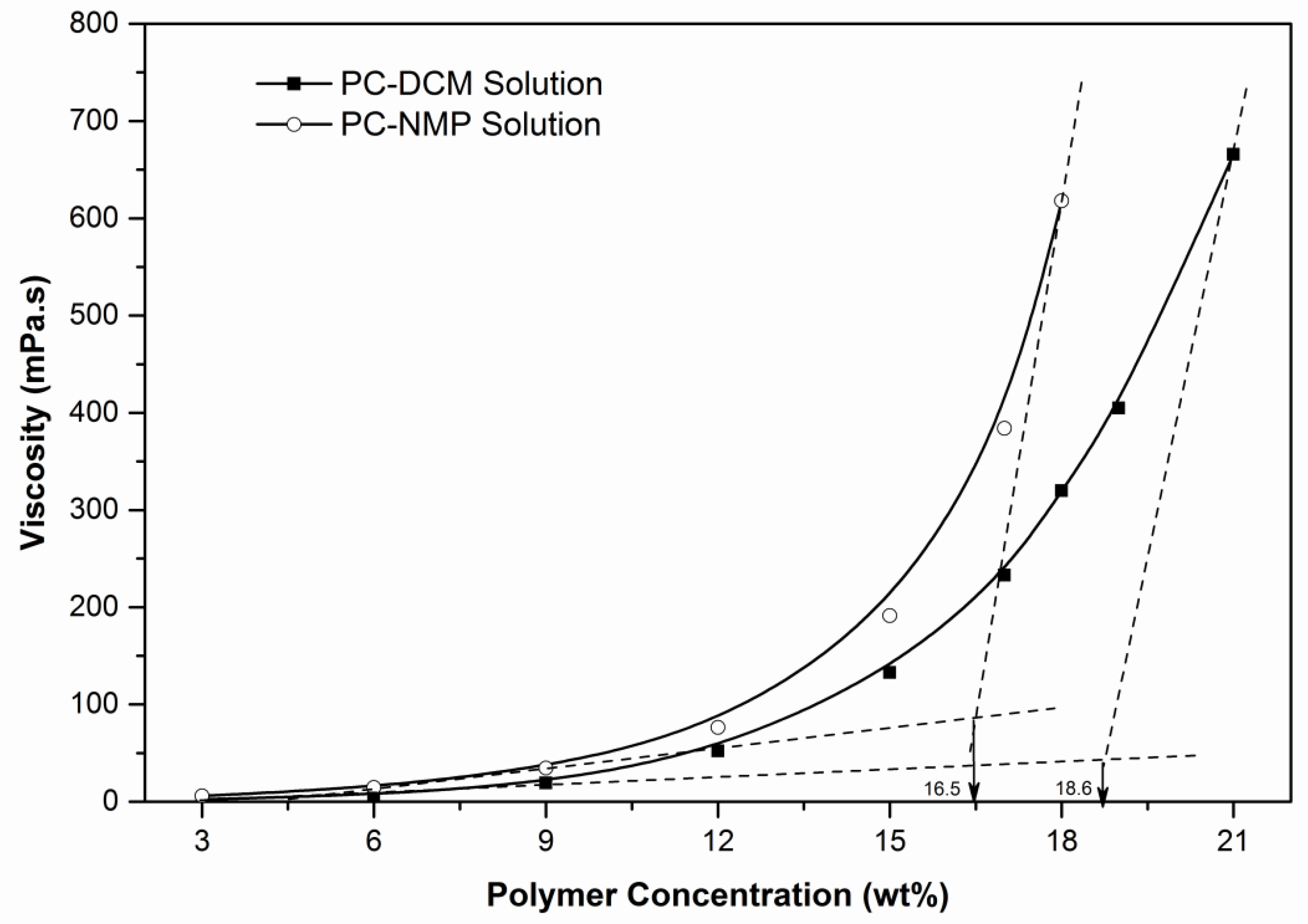
2.3. Viscosity and Density Determination
2.4. Cloud Point Determination
2.5. Preparation of PC Membranes
2.6. Characterization
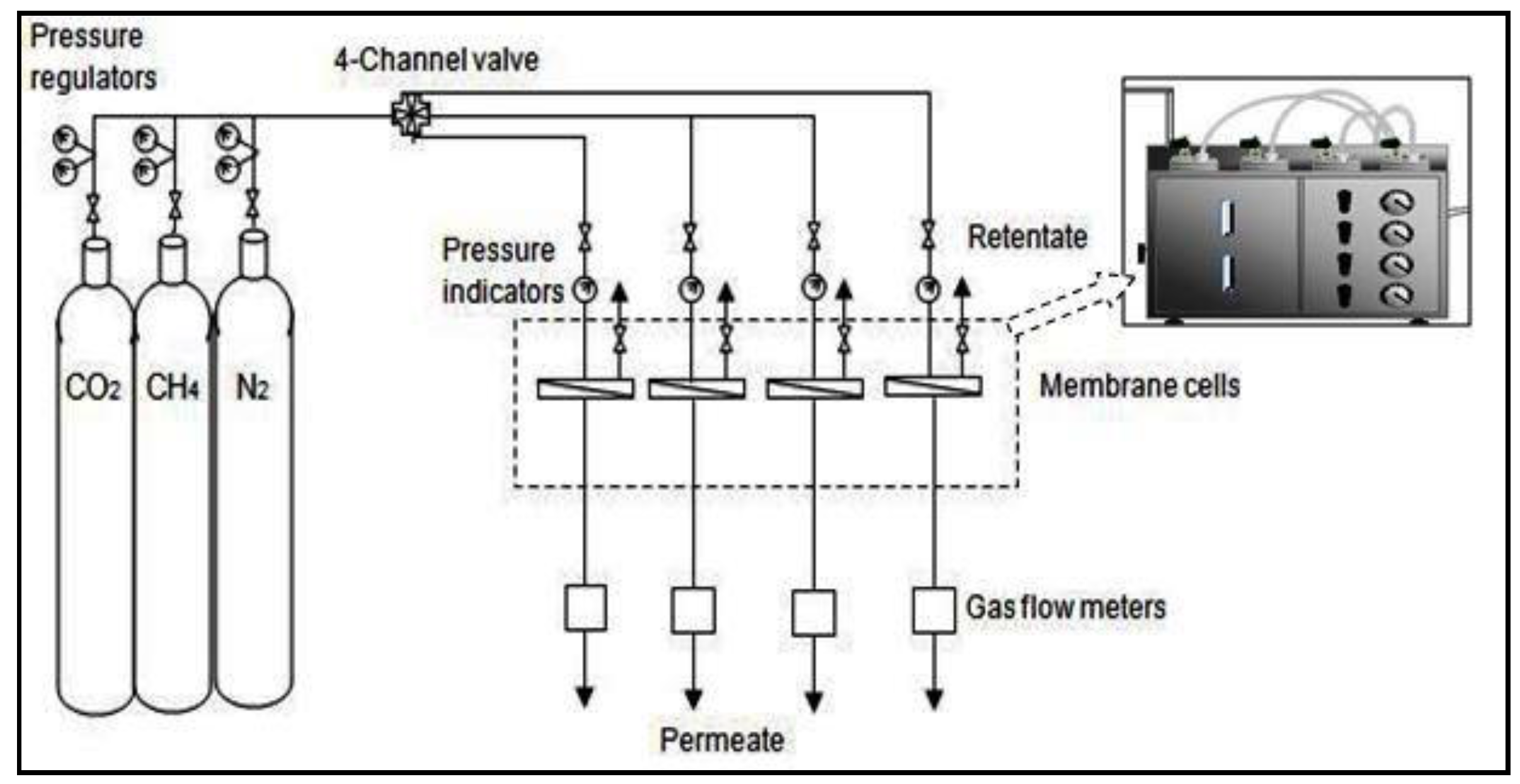
2.7. Performance Tests
2.8. Calculation of Solubility and Interaction Parameters
2.8.1. The Hansen’s Solubility Parameter
2.8.2. The Solvent/Polymer and Nonsolvent/Polymer Interaction Parameters
3. Results and Discussion
3.1. Solubility Behavior of PC
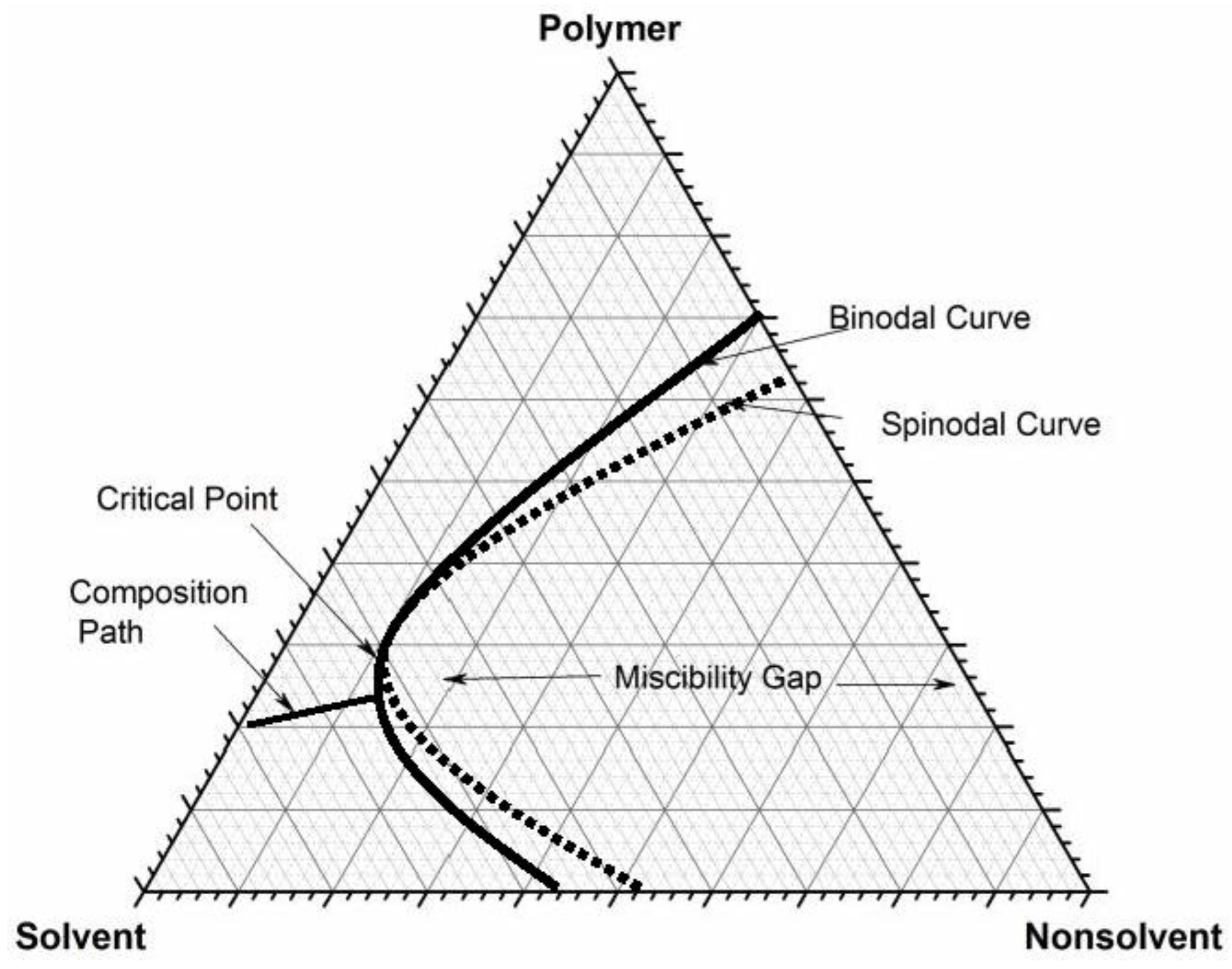
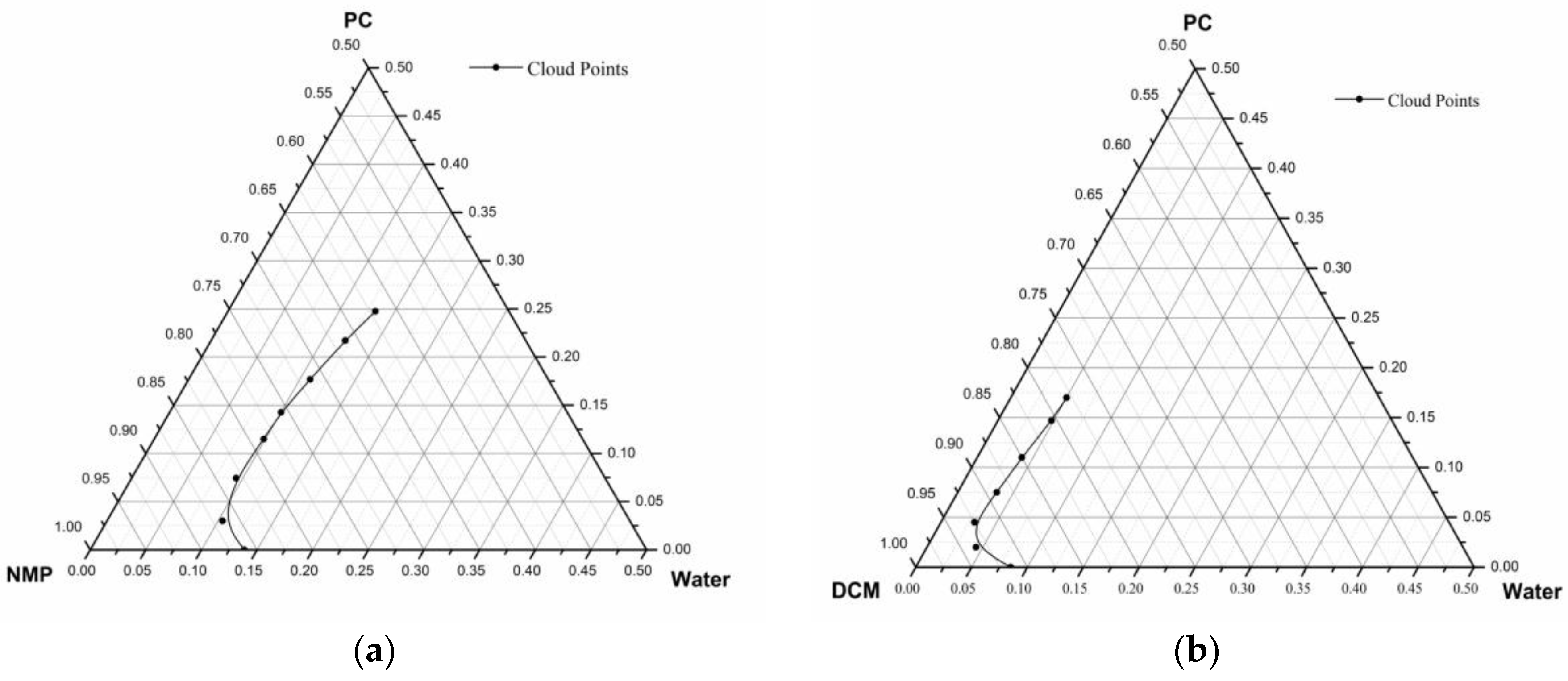
3.2. Cloud Points Binodal Curve
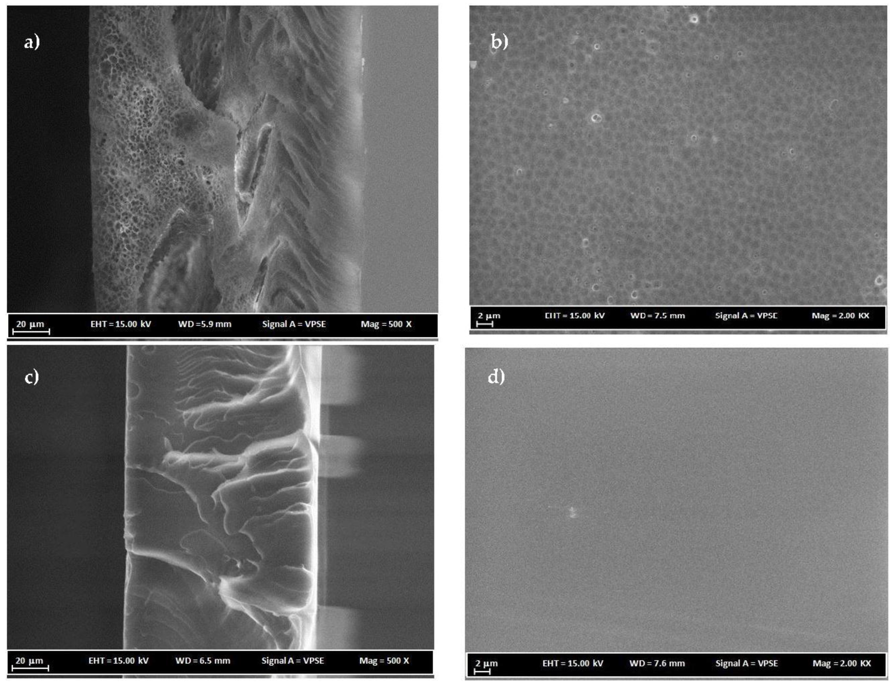
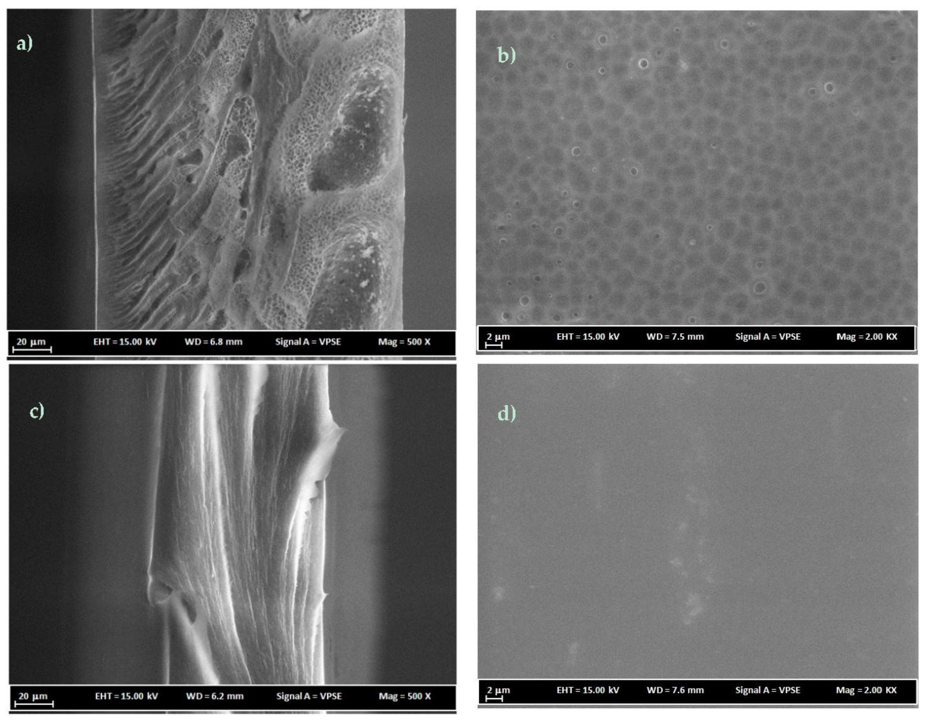
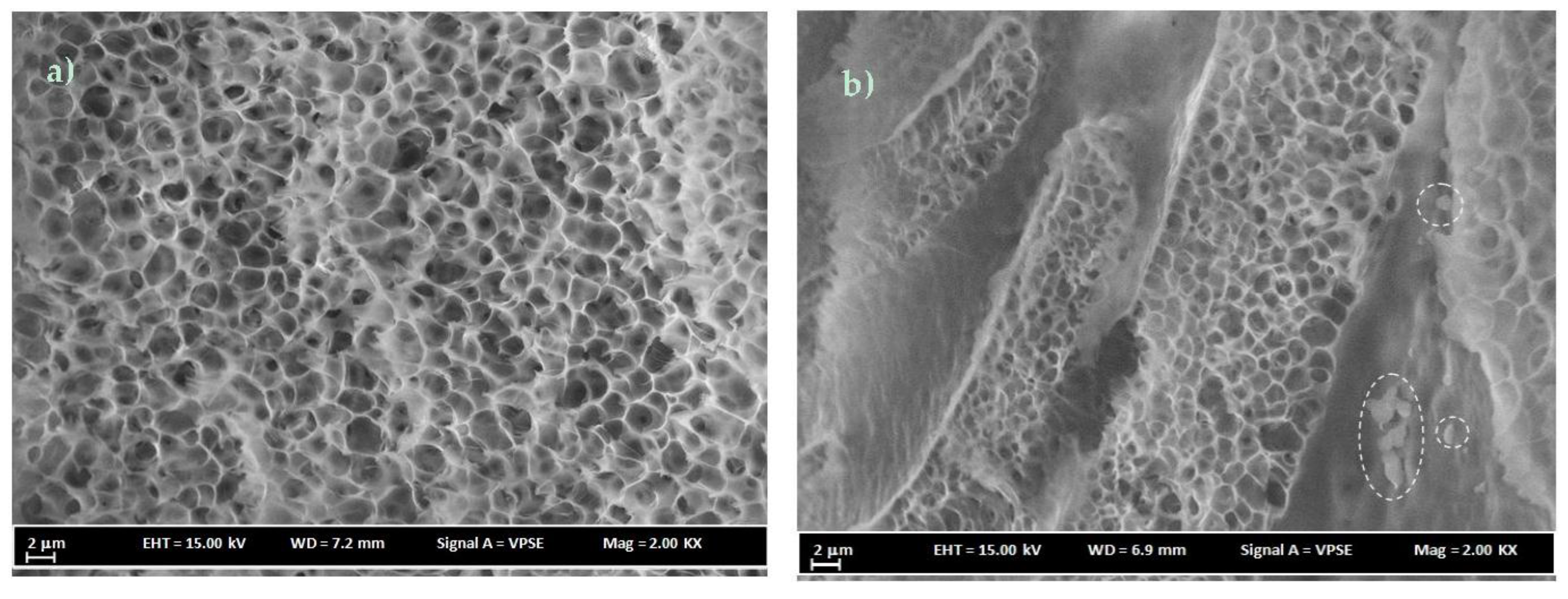
3.3. FESEM Analysis
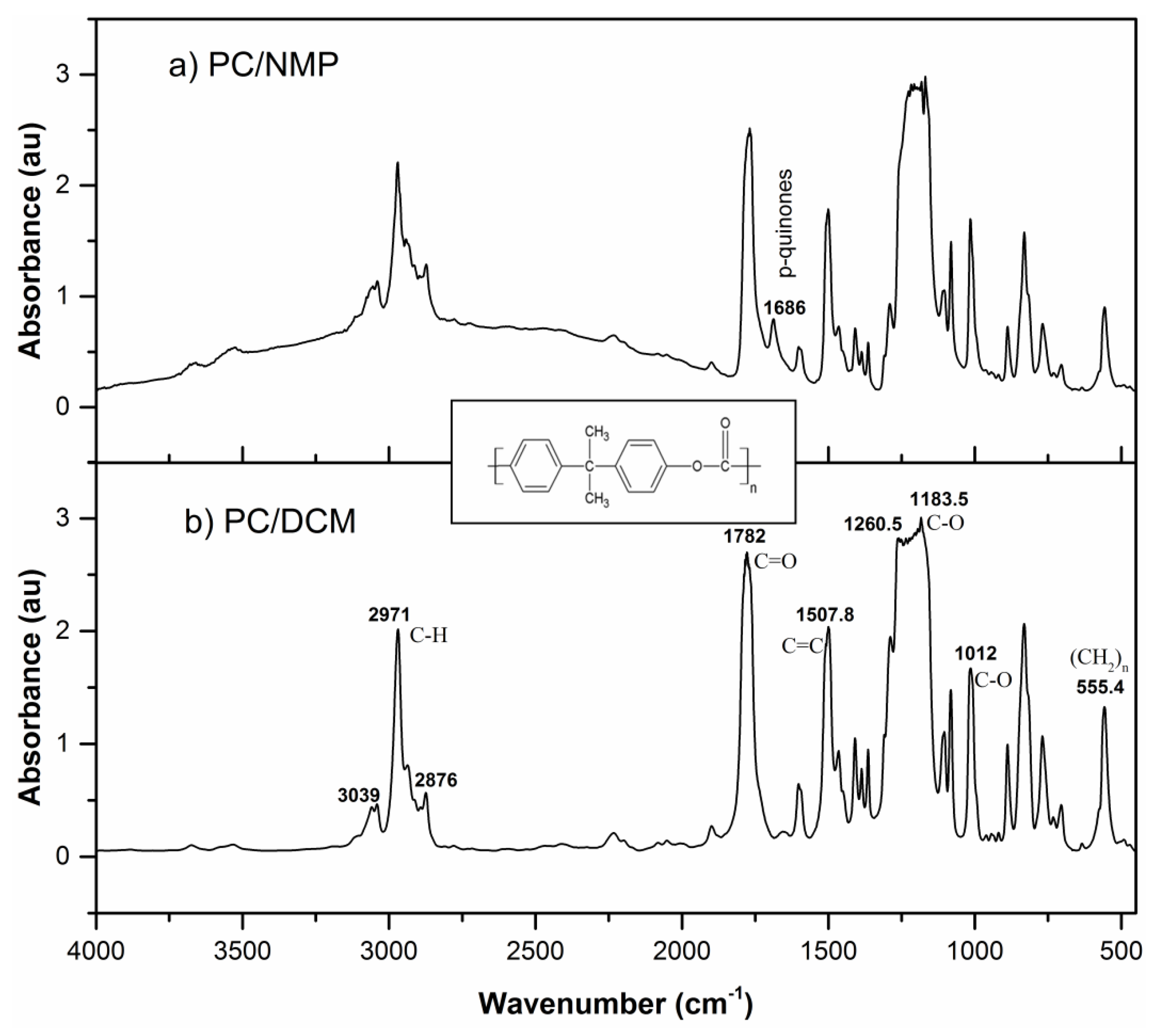
3.4. FTIR Analysis
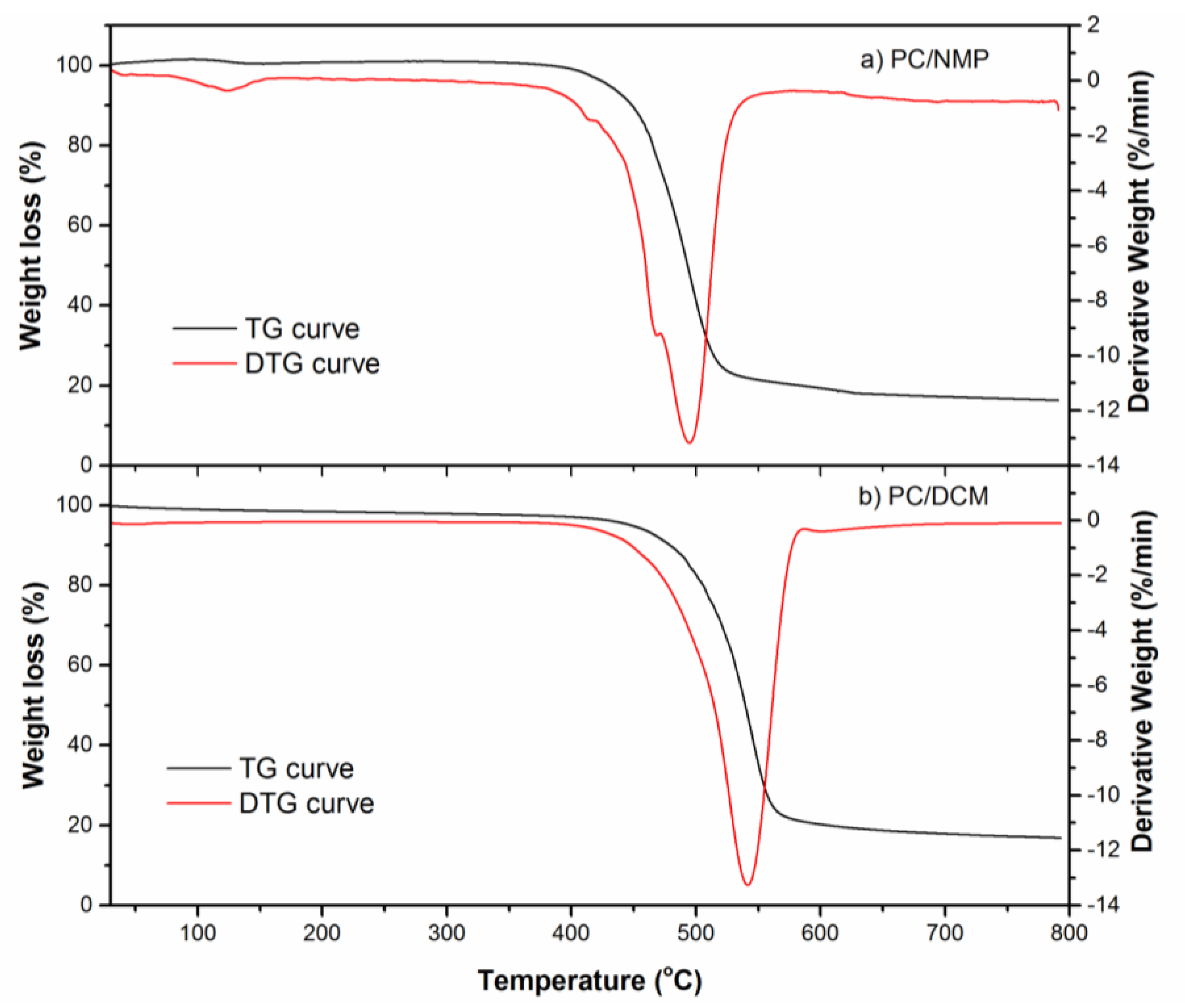
3.5. Thermal Analysis
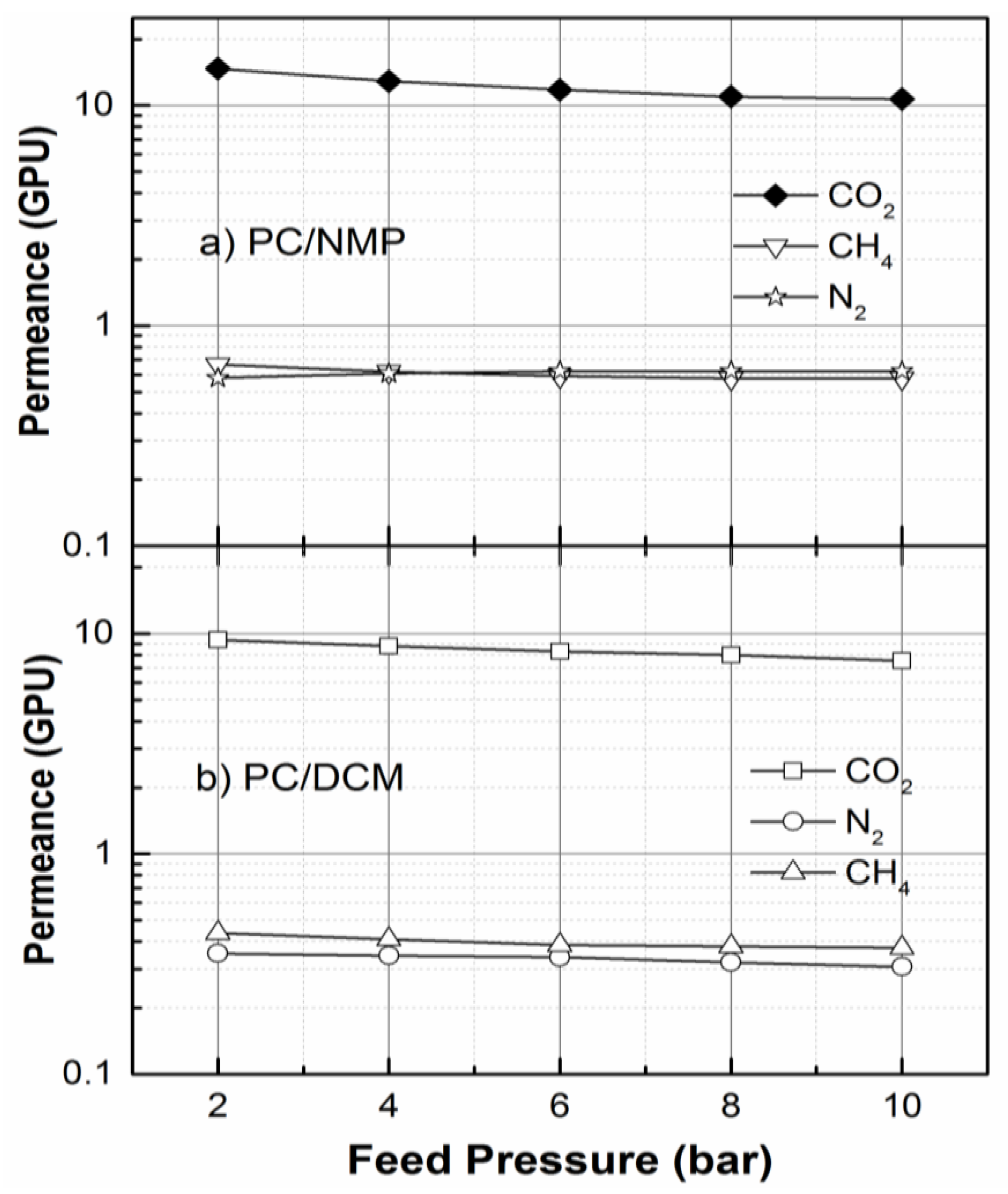
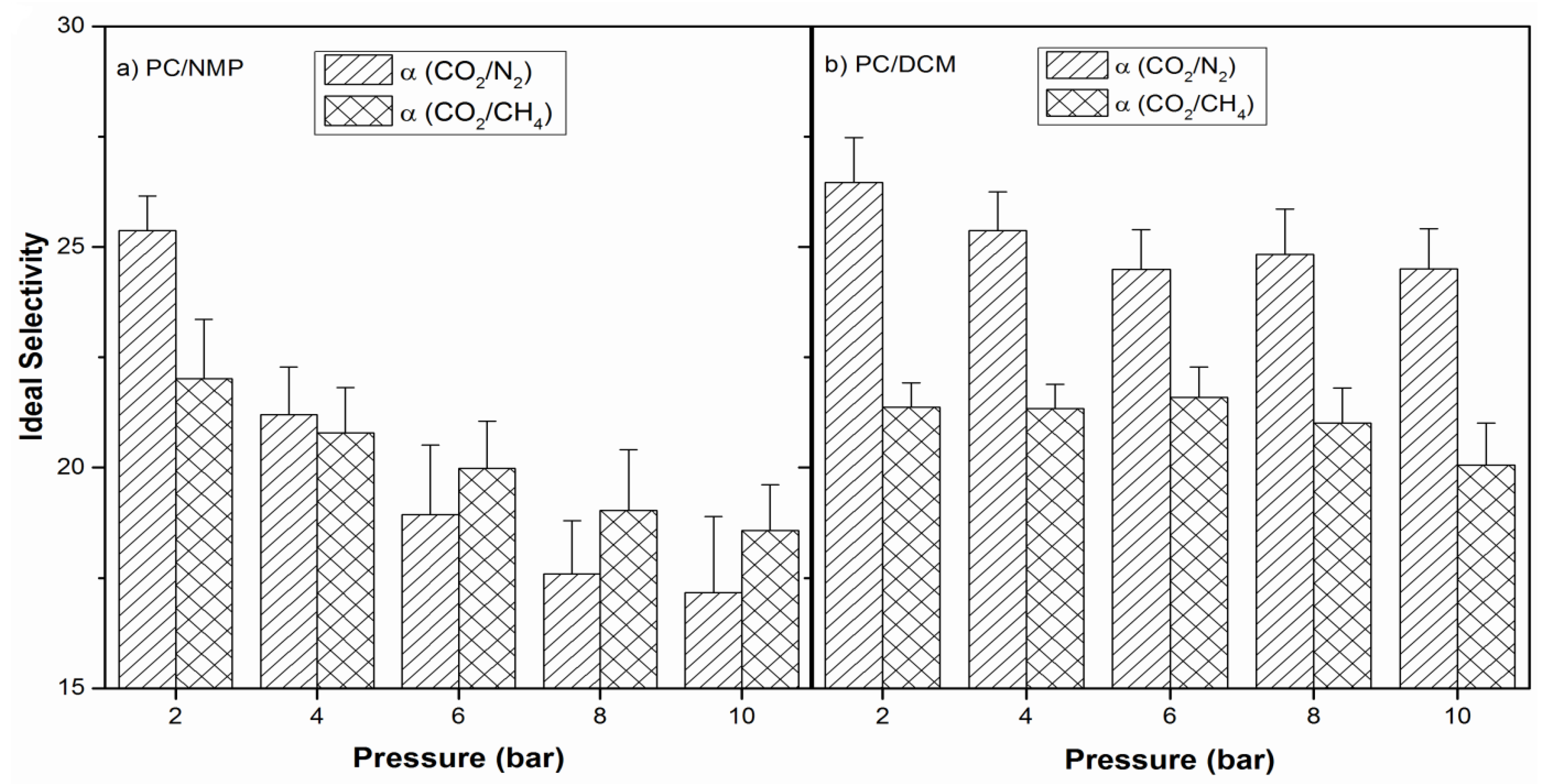
3.6. Performance Test
4. Conclusions
Acknowledgments
Author Contributions
Conflicts of Interest
Abbreviations
| PC | Bisphenol A Polycarbonate |
| DCM | Dichloromethane |
| NMP | N-Methyl-2-Pyrrolidone |
| RED | Relative Energy Difference |
| FESEM | Field Emission Scanning Electron Microscope |
| FTIR | Fourier Transform Infrared Spectroscopy |
| TGA | Thermogravimetric analyzer (or analysis) |
Greek Symbols
| v [cm3·mol−1] | The molar volume of ternary system component |
| δd [(MPa)1/2] | The dispersive component of solubility parameter |
| δh [(MPa)1/2] | The contribution due to hydrogen bonding |
| δp [(MPa)1/2] | Polar component of solubility parameter |
| δ [(MPa)1/2] | Total solubility parameter |
| χ13 | Nonsolvent/polymer interaction parameter |
| χ23 | Solvent/polymer interaction parameter |
| ∆δi–p | Solubility parameter difference |
| α | Ideal selectivity |
| Ra | Solubility parameter distance |
| Ro | Interaction radius of polymer solubility sphere |
| R | Universal gas constant |
| T | Absolute Temperature |
References
- Kim, H.; Min, B.R.; Won, J.; Park, H.C.; Kang, Y.S. Phase behavior and mechanism of membrane formation for polyimide/DMSO/water system. J. Membr. Sci. 2001, 187, 47–55. [Google Scholar] [CrossRef]
- Strathmann, H.; Kock, K. The formation mechanism of phase inversion membranes. Desalination 1977, 21, 241–255. [Google Scholar] [CrossRef]
- Luccio, M.; Nobrega, R.; Borges, C.P. Microporous anisotropic phase inversion membranes from bisphenol A polycarbonate: Effect of additives to the polymer solution. J. Appl. Polym. Sci. 2002, 86, 3085–3096. [Google Scholar] [CrossRef]
- Machado, P.S.T.; Habert, A.C.; Borges, C.P. Membrane formation mechanism based on precipitation kinetics and membrane morphology: Flat and hollow fiber polysulfone membranes. J. Membr. Sci. 1999, 155, 171–183. [Google Scholar] [CrossRef]
- Hopkinson, I.; Myatt, M. Phase Separation in Ternary Polymer Solutions Induced by Solvent Loss. Macromolecules 2002, 35, 5153–5160. [Google Scholar] [CrossRef]
- Stropnik, C.; Germic, L.; Zerjal, B. Morphology variety and formation mechanisms of polymeric membranes prepared by wet phase inversion. J. Appl. Polym. Sci. 1996, 61, 1821–1830. [Google Scholar] [CrossRef]
- Wijmans, J.G.; Kant, J.; Mulder, M.H.V.; Smolders, C.A. Phase separation phenomena in solutions of polysulfone in mixtures of a solvent and a nonsolvent: Relationship with membrane formation. Polymer 1985, 26, 1539–1546. [Google Scholar]
- Klenin, V.J. Features of Phase Separation in Polymeric Systems: Cloud-Point Curves (Discussion). Univers. J. Mater. Sci. 2013, 1, 39–45. [Google Scholar]
- Pinnau, I.; Koros, W.J. A qualitative skin layer formation mechanism for membranes made by dry/wet phase inversion. J. Polym. Sci. Part B: Polym. Phys. 1993, 31, 419–427. [Google Scholar] [CrossRef]
- Young, T.-H.; Chen, L.-W. Pore formation mechanism of membranes from phase inversion process. Desalination 1995, 103, 233–247. [Google Scholar] [CrossRef]
- Matz, R. The structure of cellulose acetate membranes 1. The development of porous structures in anisotropic membranes. Desalination 1972, 10, 1–15. [Google Scholar] [CrossRef]
- Ray, R.J.; Krantz, W.B.; Sani, R.L. Linear stability theory model for finger formation in asymmetric membranes. J. Membr. Sci. 1985, 23, 155–182. [Google Scholar] [CrossRef]
- Smolders, C.A.; Reuvers, A.J.; Boom, R.M.; Wienk, I.M. Microstructures in phase-inversion membranes. Part 1. Formation of macrovoids. J. Membr. Sci. 1992, 73, 259–275. [Google Scholar] [CrossRef]
- Hatti-Kaul, R.; Kaul, A. Aqueous Two-Phase Systems: Methods and Protocols, in Methods in Biotechnology; Humana Press Inc.: Totowa, NJ, USA, 2000; pp. 11–21. [Google Scholar]
- Iqbal, M.; Man, Z.; Mukhtar, H.; Dutta, B.K. Solvent effect on morphology and CO2/CH4 separation performance of asymmetric polycarbonate membranes. J. Membr. Sci. 2008, 318, 167–175. [Google Scholar] [CrossRef]
- Wang, D.; Li, K.; Sourirajan, S.; Teo, W.K. Phase separation phenomena of polysulfone/solvent/organic nonsolvent and polyethersulfone/solvent/organic nonsolvent systems. J. Appl. Polym. Sci. 1993, 50, 1693–1700. [Google Scholar] [CrossRef]
- Maghsoud, Z.; Famili, M.H.N.; Madaeni, S.S. Phase diagram calculations of water/tetrahydrofuran/poly (vinyl chloride) ternary system based on a compressible regular solution model. Iran. Polym. J. 2010, 19, 581–588. [Google Scholar]
- Barzin, J.; Sadatnia, B. Theoretical phase diagram calculation and membrane morphology evaluation for water/solvent/polyethersulfone systems. Polymer 2007, 48, 1620–1631. [Google Scholar] [CrossRef]
- Albo, J.; Wang, J.; Tsuru, T. Application of interfacially polymerized polyamide composite membranes to isopropanol dehydration: Effect of membrane pre-treatment and temperature. J. Membr. Sci. 2014, 453, 384–393. [Google Scholar]
- Albo, J.; Wang, J.; Tsuru, T. Gas transport properties of interfacially polymerized polyamide composite membranes under different pre-treatments and temperatures. J. Membr. Sci. 2014, 449, 109–118. [Google Scholar] [CrossRef]
- Laciak, D.; Robeson, L.; Smith, C. Group contribution modeling of gas transport in polymeric membranes. ACS Publ. 1999, 733, 151–178. [Google Scholar]
- Marrero, J.; Gani, R. Group-contribution based estimation of pure component properties. Fluid Phase Equilib. 2001, 183–184, 183–208. [Google Scholar] [CrossRef]
- Lindvig, T.; Michelsen, M.L.; Kontogeorgis, G.M. A Flory–Huggins model based on the Hansen solubility parameters. Fluid Phase Equilib. 2002, 203, 247–260. [Google Scholar] [CrossRef]
- Skaarup, K.; Hansen, C.M. The three dimensional solubility parameter—Key to paint component affinities III. J. Paint Technol. 1969, 39, 511–514. [Google Scholar]
- Miller-Chou, B.A.; Koenig, J.L. A review of polymer dissolution. Prog. Polym. Sci. 2003, 28, 1223–1270. [Google Scholar] [CrossRef]
- Guillen, G.R.; Pan, Y.; Li, M.; Hoek, M.V. Preparation and Characterization of Membranes Formed by Nonsolvent Induced Phase Separation: A Review. Ind. Eng. Chem. Res. 2011, 50, 3798–3817. [Google Scholar] [CrossRef]
- Hansen, C.M. Hansen Solubility Parameters: A User’s Handbook; CRC Press: Boca Raton, FL, USA, 2000. [Google Scholar]
- Wei, Y.-M.; Xu, Z.-L.; Yang, X.-T.; Liu, H.-L. Mathematical calculation of binodal curves of a polymer/solvent/nonsolvent system in the phase inversion process. Desalination 2006, 192, 91–104. [Google Scholar] [CrossRef]
- Ahmed, I.; Idris, A.; Hussain, A.; Yusof, Z.A.M.; Saad Kahn, M. Influence of Co-Solvent Concentration on the Properties of Dope Solution and Performance of Polyethersulfone Membranes. Chem. Eng. Technol. 2013, 36, 1683–1690. [Google Scholar] [CrossRef]
- Xing, D.Y.; Peng, N.; Chung, T.-S. Formation of Cellulose Acetate Membranes via Phase Inversion Using Ionic Liquid, [BMIM] SCN, As the Solvent. Ind. Eng. Chem. Res. 2010, 49, 8761–8769. [Google Scholar] [CrossRef]
- Bakeri, G.; Ismail, A.F.; Shariaty-Niassar, M.; Matsuura, T. Effect of polymer concentration on the structure and performance of polyetherimide hollow fiber membranes. J. Membr. Sci. 2010, 363, 103–111. [Google Scholar] [CrossRef]
- Coates, J. (Ed.) Interpretation of Infrared Spectra, a Practical Approach, in Encyclopedia of Analytical Chemistry; John Wiley & Sons: Chichester, UK, 2000; pp. 10815–10837. [Google Scholar]
- Socrates, G. Infrared and Raman Characteristic Group Frequencies: Tables and Charts; John Wiley & Sons Ltd.: Chichester, UK, 2001. [Google Scholar]
- Stuart, B. Infrared Spectroscopy: Fundamentals and Applications; John Wiley & Sons Ltd.: Chichester, UK, 2004. [Google Scholar]
- Zhang, L.; Fang, W.; Jiang, J. Effects of Residual Solvent on Membrane Structure and Gas Permeation in a Polymer of Intrinsic Microporosity: Insight from Atomistic Simulation. J. Phys. Chem. C 2011, 115, 11233–11239. [Google Scholar] [CrossRef]
- Albo, J.; Hagiwara, H.; Yanagishita, H.; Ito, K.; Tsuru, T. Structural Characterization of Thin-Film Polyamide Reverse Osmosis Membranes. Ind. Eng. Chem. Res. 2014, 53, 1442–1451. [Google Scholar] [CrossRef]
- Koros, W.J.; Fleming, G.K. Membrane-based gas separation. J. Membr. Sci. 1993, 83, 1–80. [Google Scholar] [CrossRef]


| Material | PC | NMP | DCM | Water |
|---|---|---|---|---|
| Vm (mol/cc) | 211.67 | 96.50 | 63.9 | 18.02 |
| δd (MPa)1/2 | 17.95 | 18.00 | 18.2 | 15.50 |
| δp (MPa)1/2 | 3.16 | 12.30 | 6.30 | 16.00 |
| δh (MPa)1/2 | 6.87 | 7.20 | 6.10 | 42.40 |
| δ (MPa)1/2 | 19.48 | 22.96 | 20.20 | 47.90 |
| ∆δj−p | – | 9.15 | 3.24 | 37.86 |
| Ra | 12.10 | 9.14 | 3.27 | 38. 09 |
| RED | – | 0.76 | 0.27 | 3.15 |
| χ23 | – | 1.79 | 0.23 | 31.00 |
| Polymer Concentration wt % | PC-NMP | Polymer Concentration wt % | PC-DCM | ||||
|---|---|---|---|---|---|---|---|
| Density g/cm3 | Viscosity mPa·s | Refractive Index | Density g/cm3 | Viscosity mPa·s | Refractive Index | ||
| 3 | 1.043 | 5.821 | 1.474 | 3 | 1.315 | 2.431 | 1.428 |
| 6 | 1.045 | 14.509 | 1.477 | 6 | 1.313 | 7.071 | 1.435 |
| 9 | 1.056 | 34.358 | 1.481 | 9 | 1.312 | 19.283 | 1.442 |
| 12 | 1.062 | 76.376 | 1.485 | 12 | 1.311 | 52.170 | 1.450 |
| 15 | 1.068 | 191.223 | 1.489 | 15 | 1.308 | 132.822 | 1.454 |
| 17 | 1.071 | 384.214 | 1.492 | 17 | 1.309 | 232.856 | 1.459 |
| 18 | 1.078 | 617.930 | 1.498 | 19 | 1.304 | 404.968 | 1.466 |
| – | – | – | – | 21 | 1.306 | 665.786 | 1.469 |
| S. No. | Membrane Name | Degradation Temperature °C | Residue % | |
|---|---|---|---|---|
| Tonset | Tmax | |||
| 1 | PC/NMP membrane | 430.26 | 495.12 | 16.91 |
| 2 | PC/DCM membrane | 448.26 | 540.5 | 17.2 |
© 2017 by the authors. Licensee MDPI, Basel, Switzerland. This article is an open access article distributed under the terms and conditions of the Creative Commons Attribution (CC BY) license (http://creativecommons.org/licenses/by/4.0/).
Share and Cite
Idris, A.; Man, Z.; Maulud, A.S.; Khan, M.S. Effects of Phase Separation Behavior on Morphology and Performance of Polycarbonate Membranes. Membranes 2017, 7, 21. https://doi.org/10.3390/membranes7020021
Idris A, Man Z, Maulud AS, Khan MS. Effects of Phase Separation Behavior on Morphology and Performance of Polycarbonate Membranes. Membranes. 2017; 7(2):21. https://doi.org/10.3390/membranes7020021
Chicago/Turabian StyleIdris, Alamin, Zakaria Man, Abdulhalim S. Maulud, and Muhammad Saad Khan. 2017. "Effects of Phase Separation Behavior on Morphology and Performance of Polycarbonate Membranes" Membranes 7, no. 2: 21. https://doi.org/10.3390/membranes7020021
APA StyleIdris, A., Man, Z., Maulud, A. S., & Khan, M. S. (2017). Effects of Phase Separation Behavior on Morphology and Performance of Polycarbonate Membranes. Membranes, 7(2), 21. https://doi.org/10.3390/membranes7020021