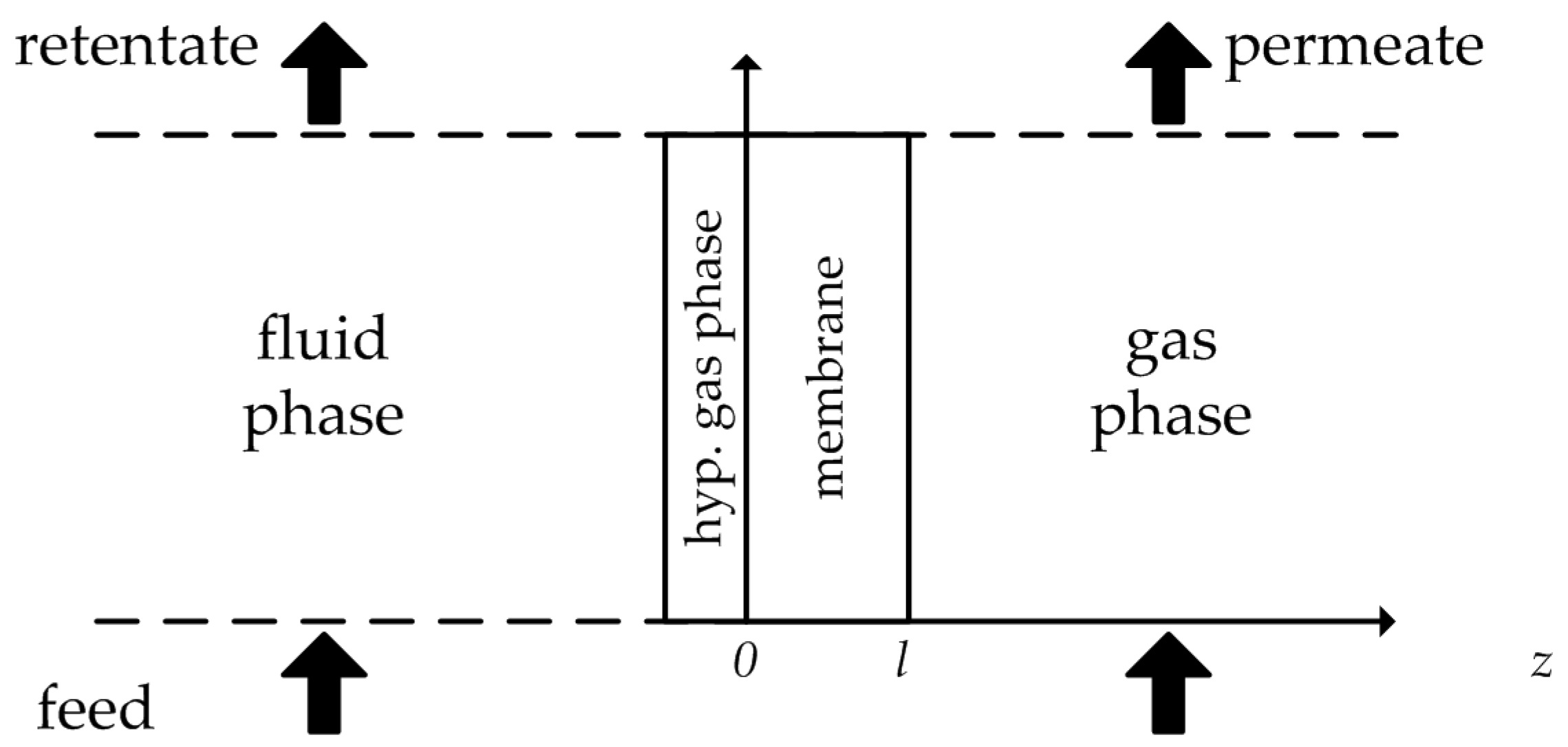
Figure 1.
Hypothetical gas phase between feed solution and membrane. Illustration adapted from [
6].
Figure 1.
Hypothetical gas phase between feed solution and membrane. Illustration adapted from [
6].
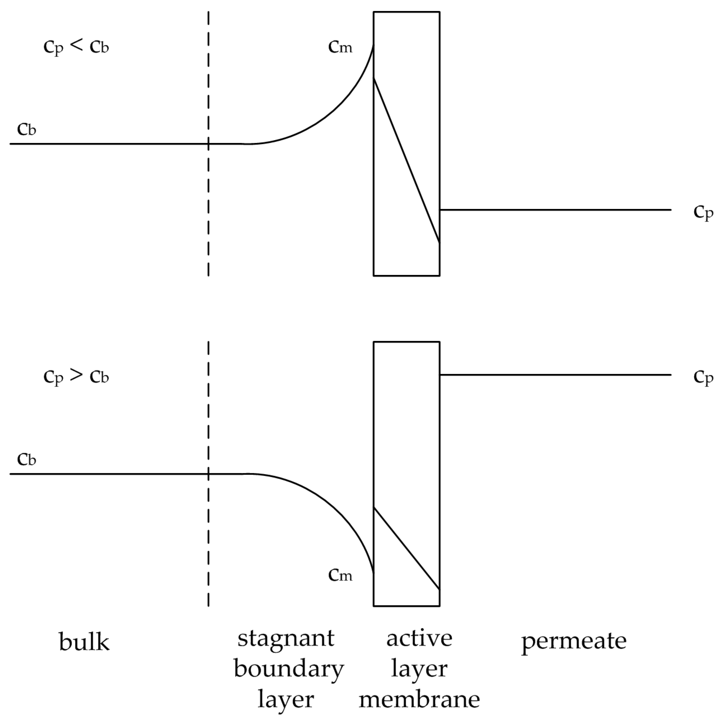
Figure 2.
Illustration of the concentration polarization effect for an accumulating substance (above) and a depleting substance (below). Adapted from [
17].
Figure 2.
Illustration of the concentration polarization effect for an accumulating substance (above) and a depleting substance (below). Adapted from [
17].
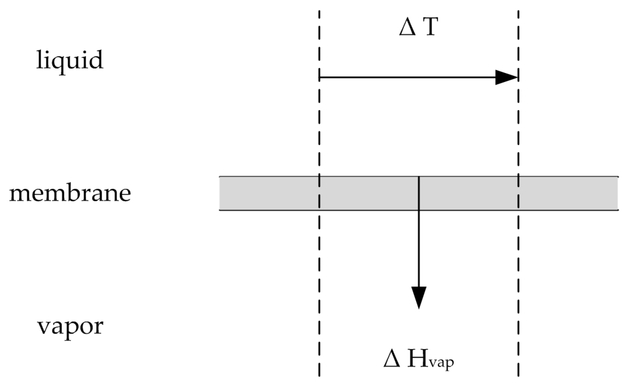
Figure 3.
Illustration of the heat transfer via vaporization. Adapted from [
21].
Figure 3.
Illustration of the heat transfer via vaporization. Adapted from [
21].
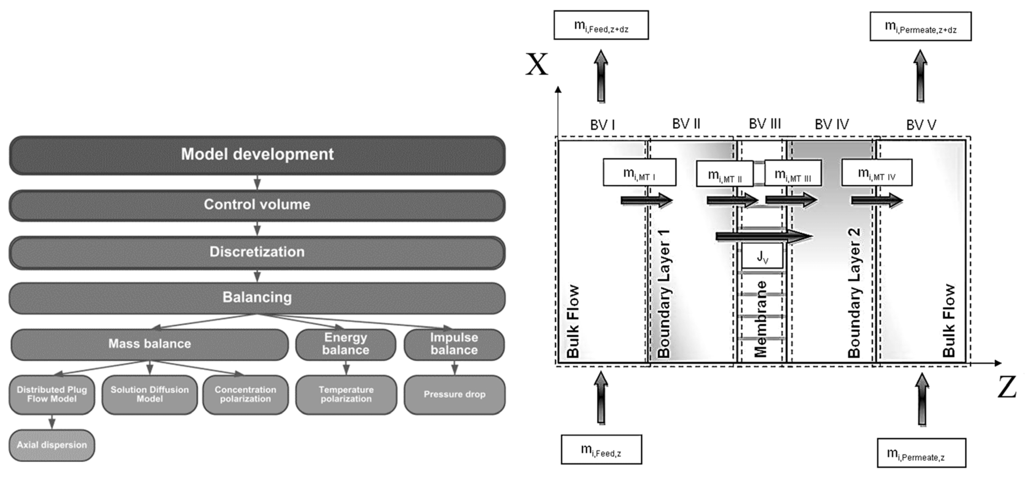
Figure 4.
Left: Course of action used for the pervaporation model development.
Right: Overview of the five control volumes used in modelling and simulation. Adapted from [
23].
Figure 4.
Left: Course of action used for the pervaporation model development.
Right: Overview of the five control volumes used in modelling and simulation. Adapted from [
23].
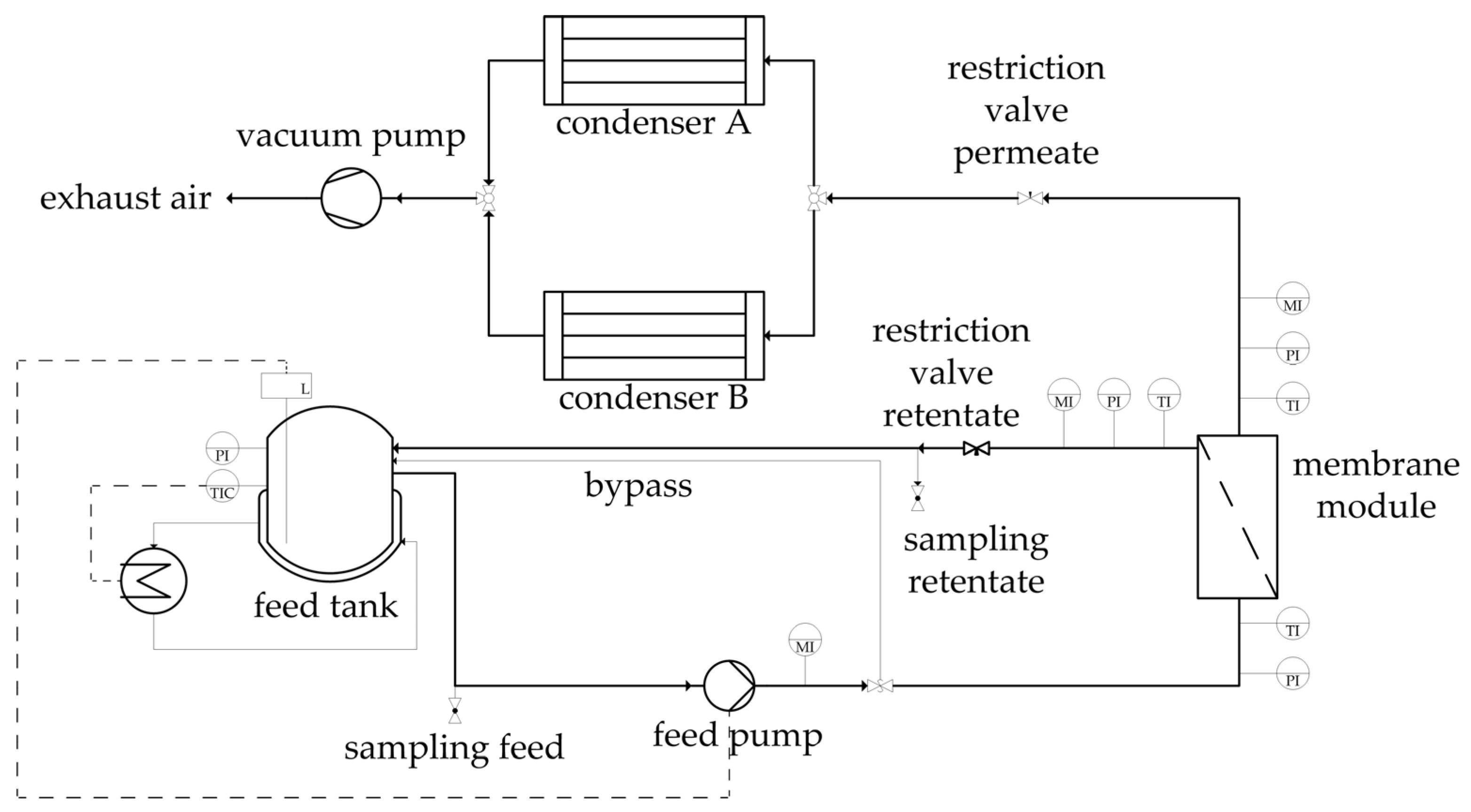
Figure 5.
Flowsheet of the pervaporation unit utilized for the binary and ternary experiments.
Figure 5.
Flowsheet of the pervaporation unit utilized for the binary and ternary experiments.
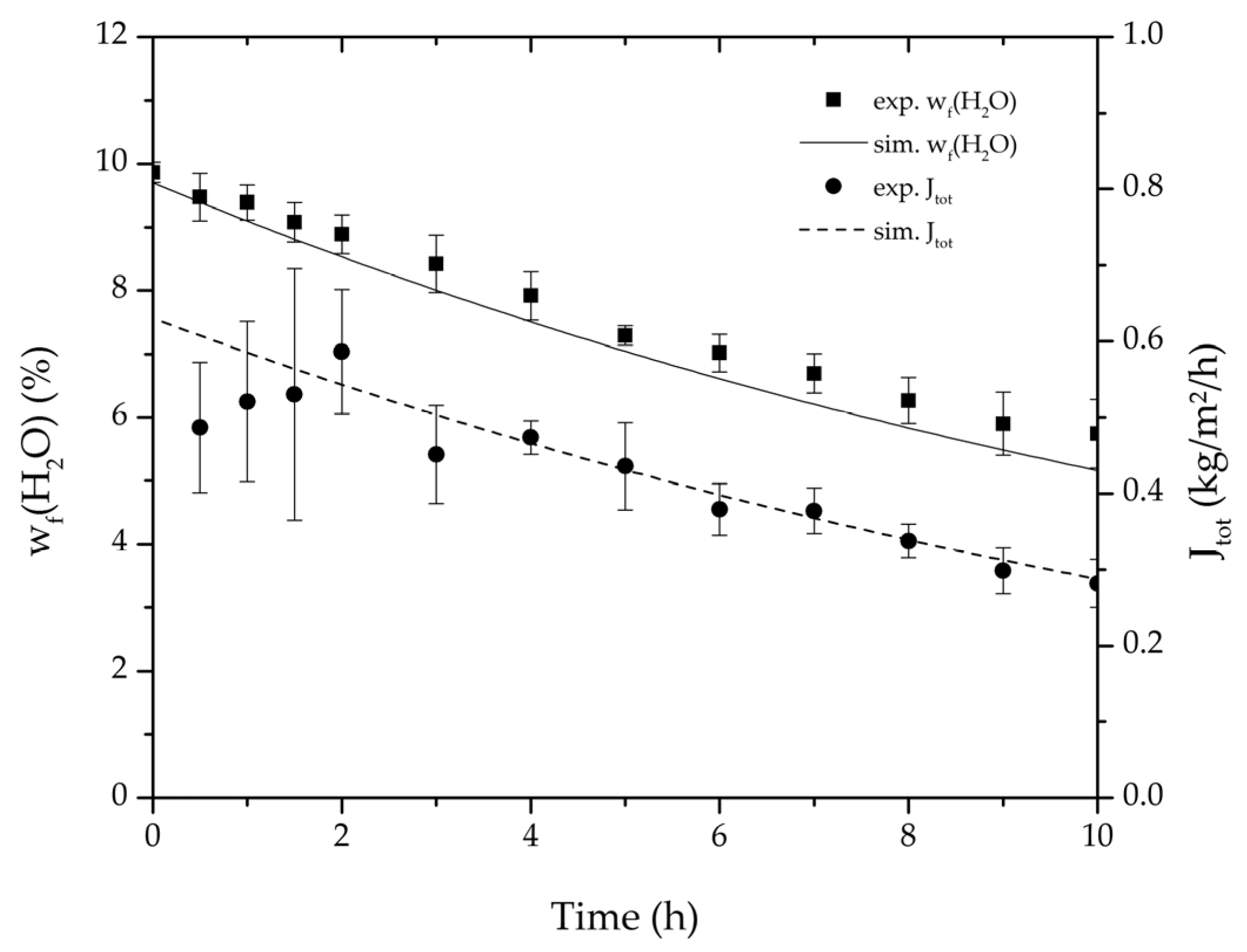
Figure 6.
Average water mass fraction of the feed and total permeate flux of the thrice-repeated centre point experiments over the experimental duration for the binary system ethanol/water. The error bars represent the standard deviation, the line the simulation result.
Figure 6.
Average water mass fraction of the feed and total permeate flux of the thrice-repeated centre point experiments over the experimental duration for the binary system ethanol/water. The error bars represent the standard deviation, the line the simulation result.
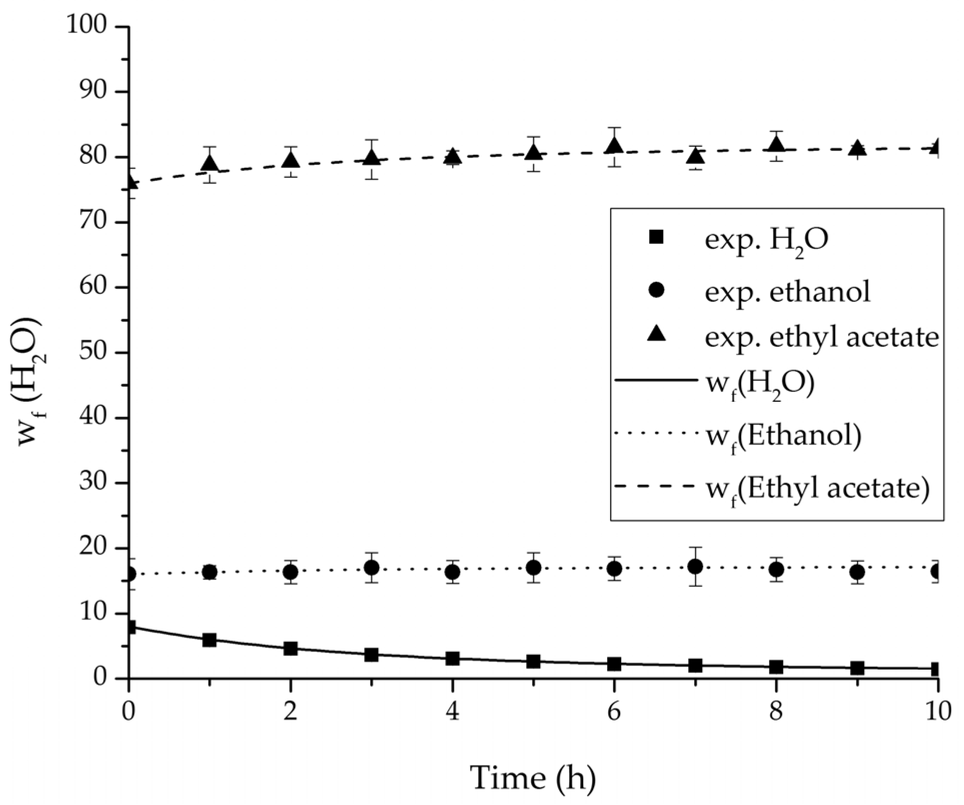
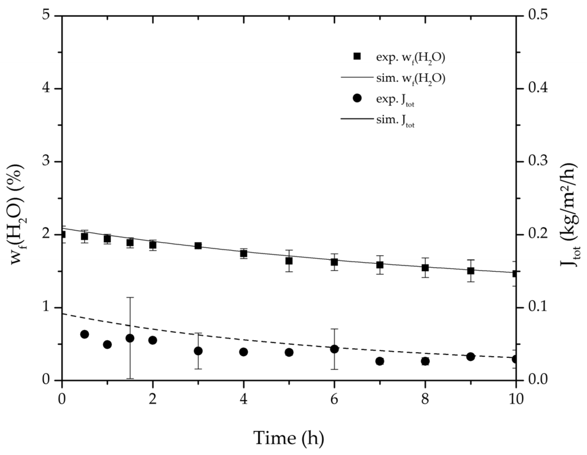
Figure 7.
Average water mass fraction of the feed and total permeate flux of the thrice-repeated centre point experiments over the experimental duration for the binary system ethyl acetate/water. The error bars represent the standard deviation, the line the simulation result.
Figure 7.
Average water mass fraction of the feed and total permeate flux of the thrice-repeated centre point experiments over the experimental duration for the binary system ethyl acetate/water. The error bars represent the standard deviation, the line the simulation result.
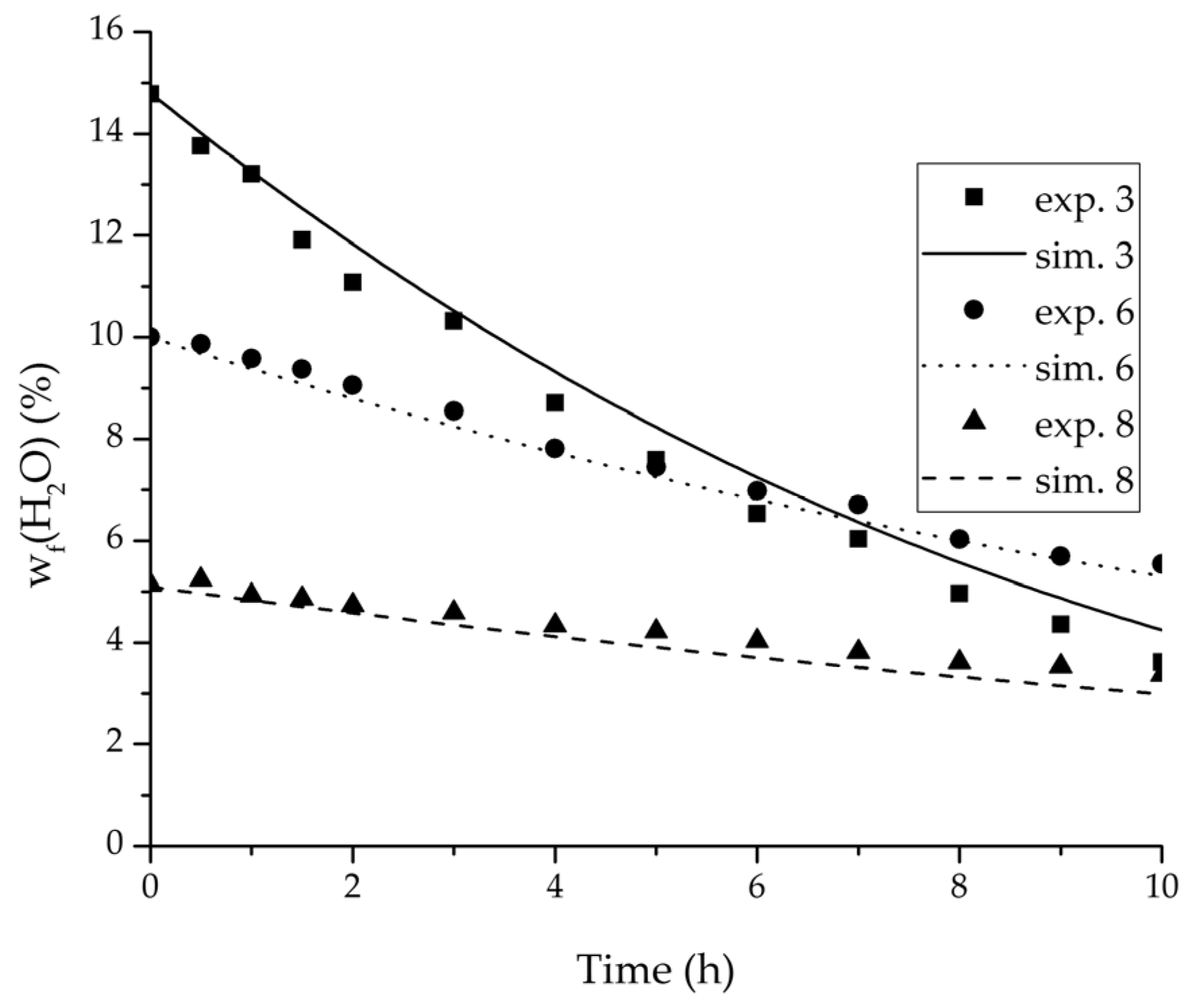
Figure 8.
Experimental water mass fractions (feed) over time for three experiments used for the validation of the permeance function for ethanol/water compared with the corresponding simulation result.
Figure 8.
Experimental water mass fractions (feed) over time for three experiments used for the validation of the permeance function for ethanol/water compared with the corresponding simulation result.
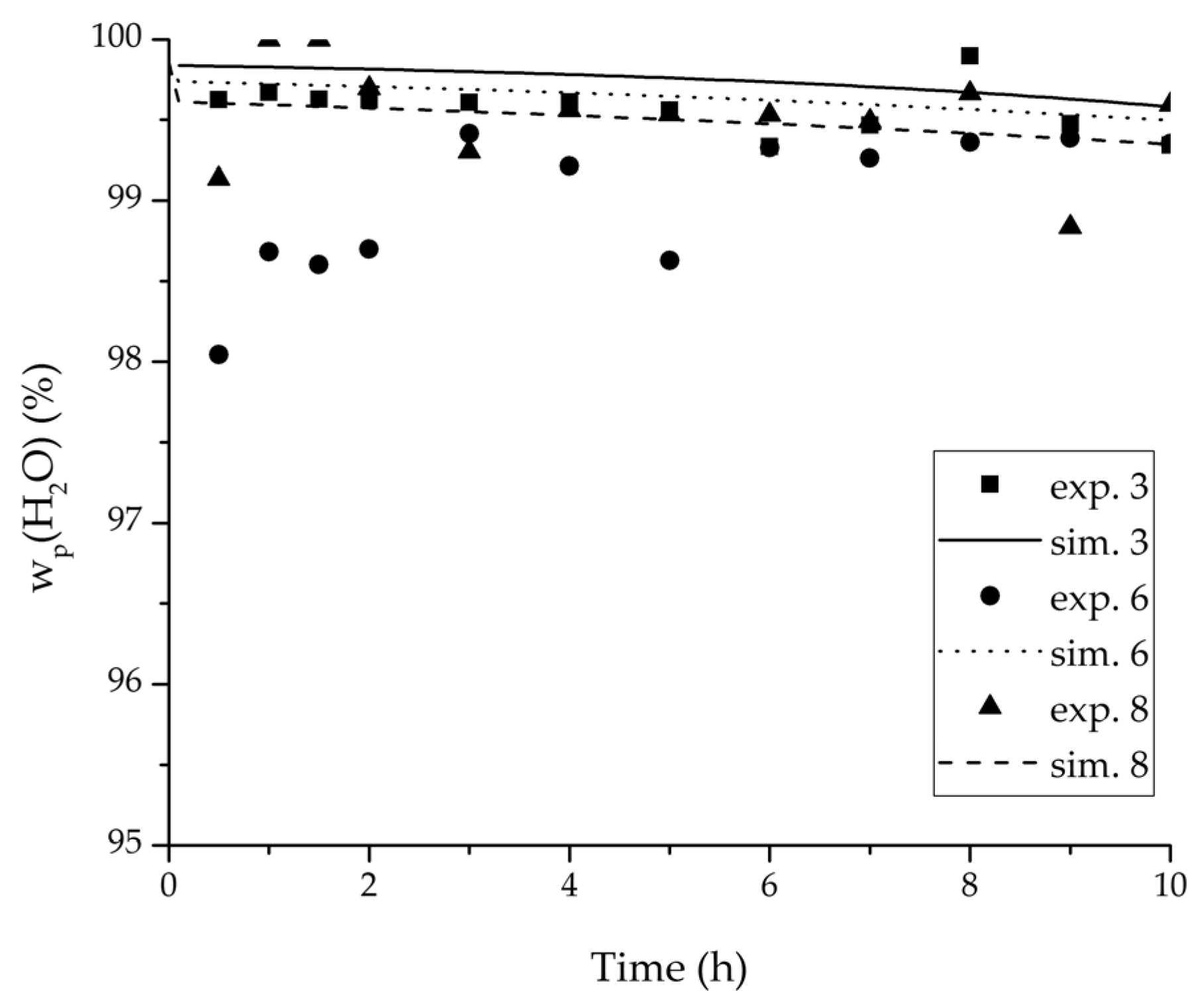
Figure 9.
Experimental water mass fractions (permeate) over time for three experiments used for the validation of the permeance function for ethanol/water compared with the corresponding simulation result.
Figure 9.
Experimental water mass fractions (permeate) over time for three experiments used for the validation of the permeance function for ethanol/water compared with the corresponding simulation result.
Figure 10.
Experimental water flux over time for three experiments used for the validation of the permeance function for ethanol/water compared with the corresponding simulation result.
Figure 10.
Experimental water flux over time for three experiments used for the validation of the permeance function for ethanol/water compared with the corresponding simulation result.
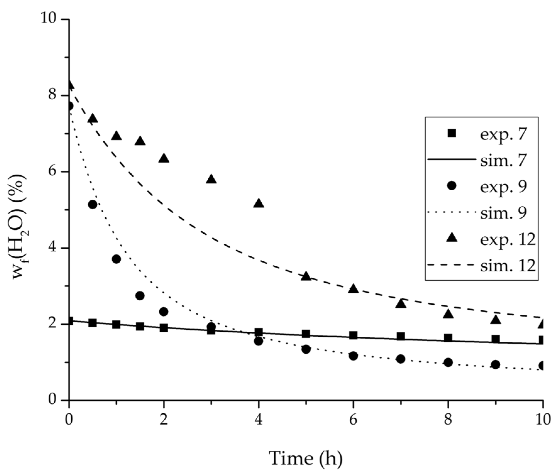
Figure 11.
Experimental water mass fractions (feed) over time for three experiments used for the validation of the permeance function for ethyl acetate/water compared with the corresponding simulation result.
Figure 11.
Experimental water mass fractions (feed) over time for three experiments used for the validation of the permeance function for ethyl acetate/water compared with the corresponding simulation result.
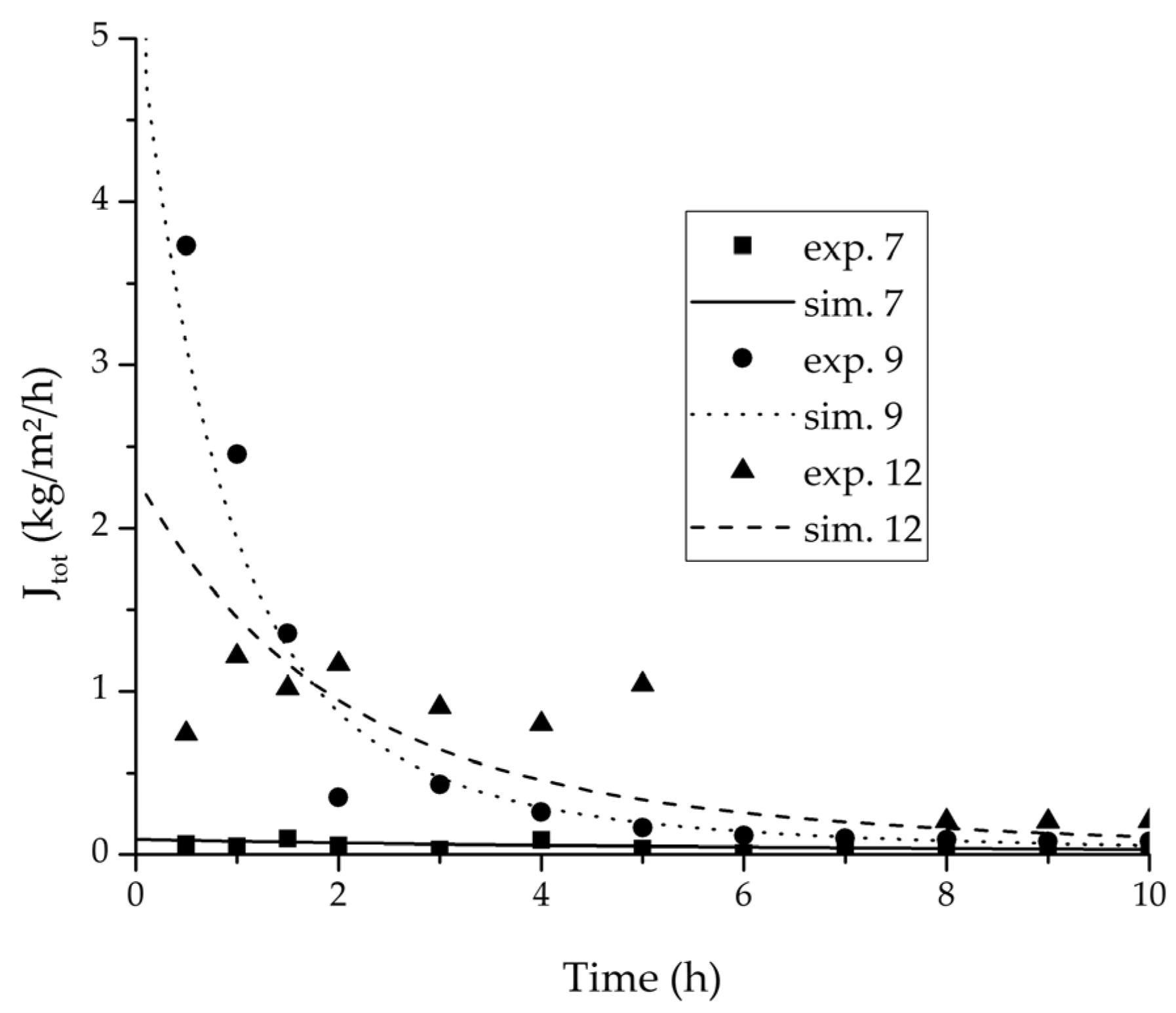
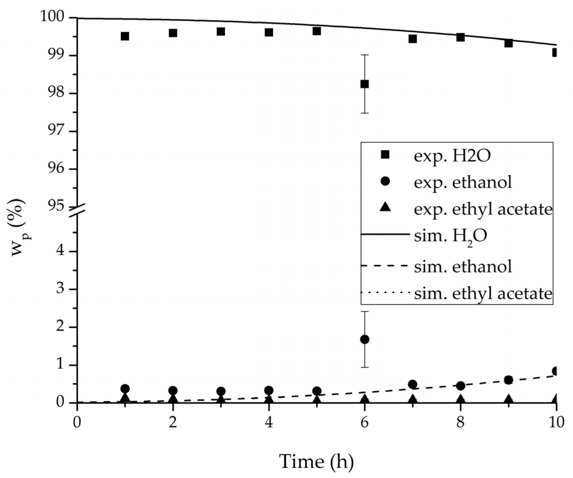
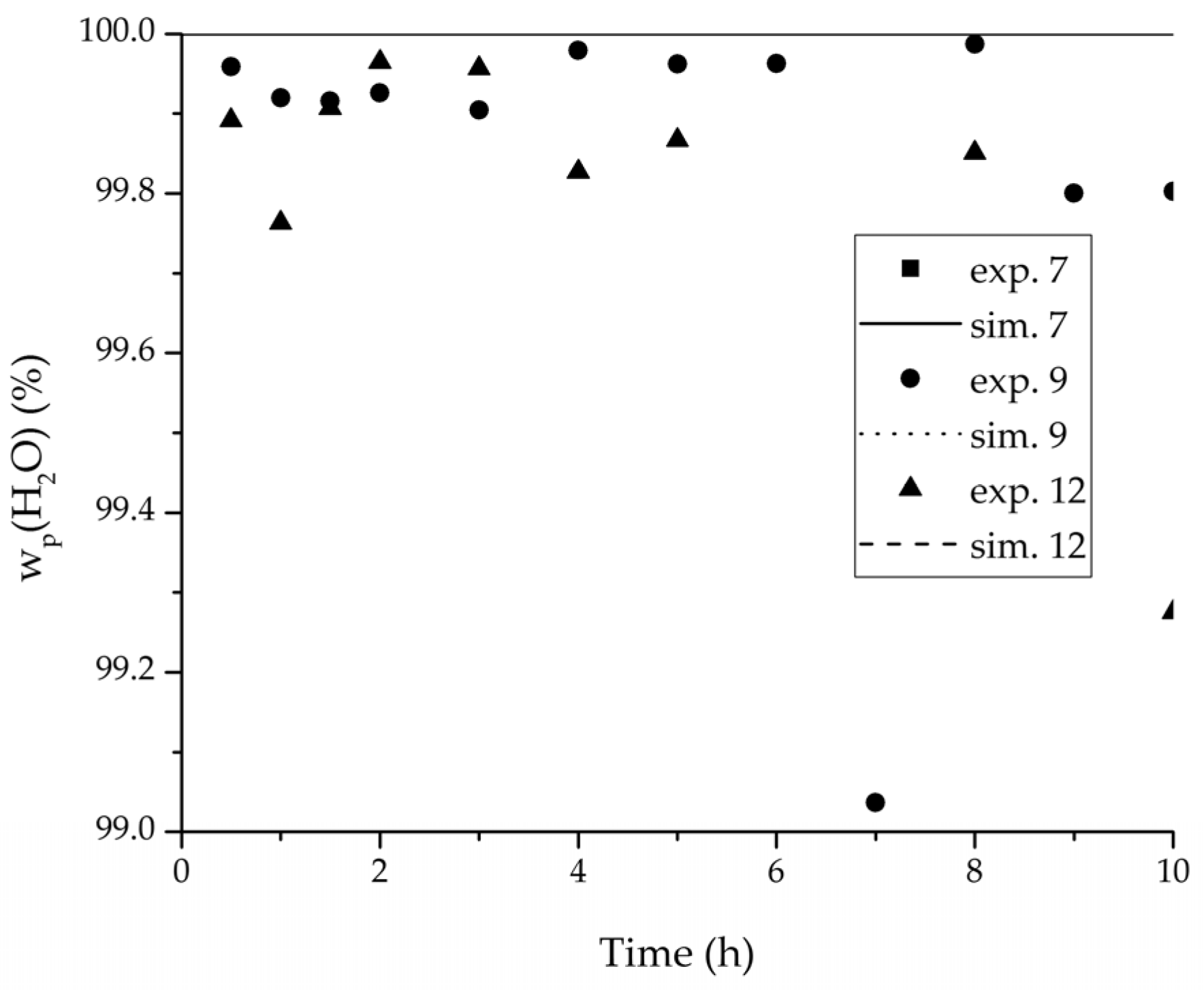
Figure 12.
Experimental water mass fractions (permeate) over time for three experiments used for the validation of the permeance function for ethyl acetate/water compared with the corresponding simulation result. All simulation curves are very close to a value of 100%. The flux of exp. 7 was too small to be analysed.
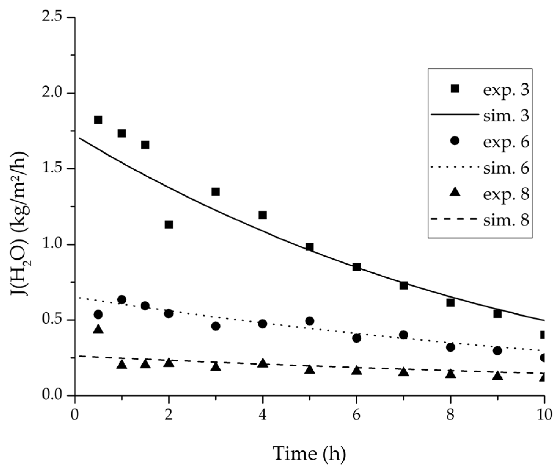
Figure 13.
Experimental water flux over time for three experiments used for the validation of the permeance function for ethyl acetate/water compared with the corresponding simulation result.
Figure 13.
Experimental water flux over time for three experiments used for the validation of the permeance function for ethyl acetate/water compared with the corresponding simulation result.
Figure 14.
Experimental and simulation feed mass fraction for the ternary system at 95 °C feed temperature.
Figure 14.
Experimental and simulation feed mass fraction for the ternary system at 95 °C feed temperature.
Figure 15.
Experimental and simulation permeate mass fractions for the ternary system at 95 °C feed temperature.
Figure 15.
Experimental and simulation permeate mass fractions for the ternary system at 95 °C feed temperature.
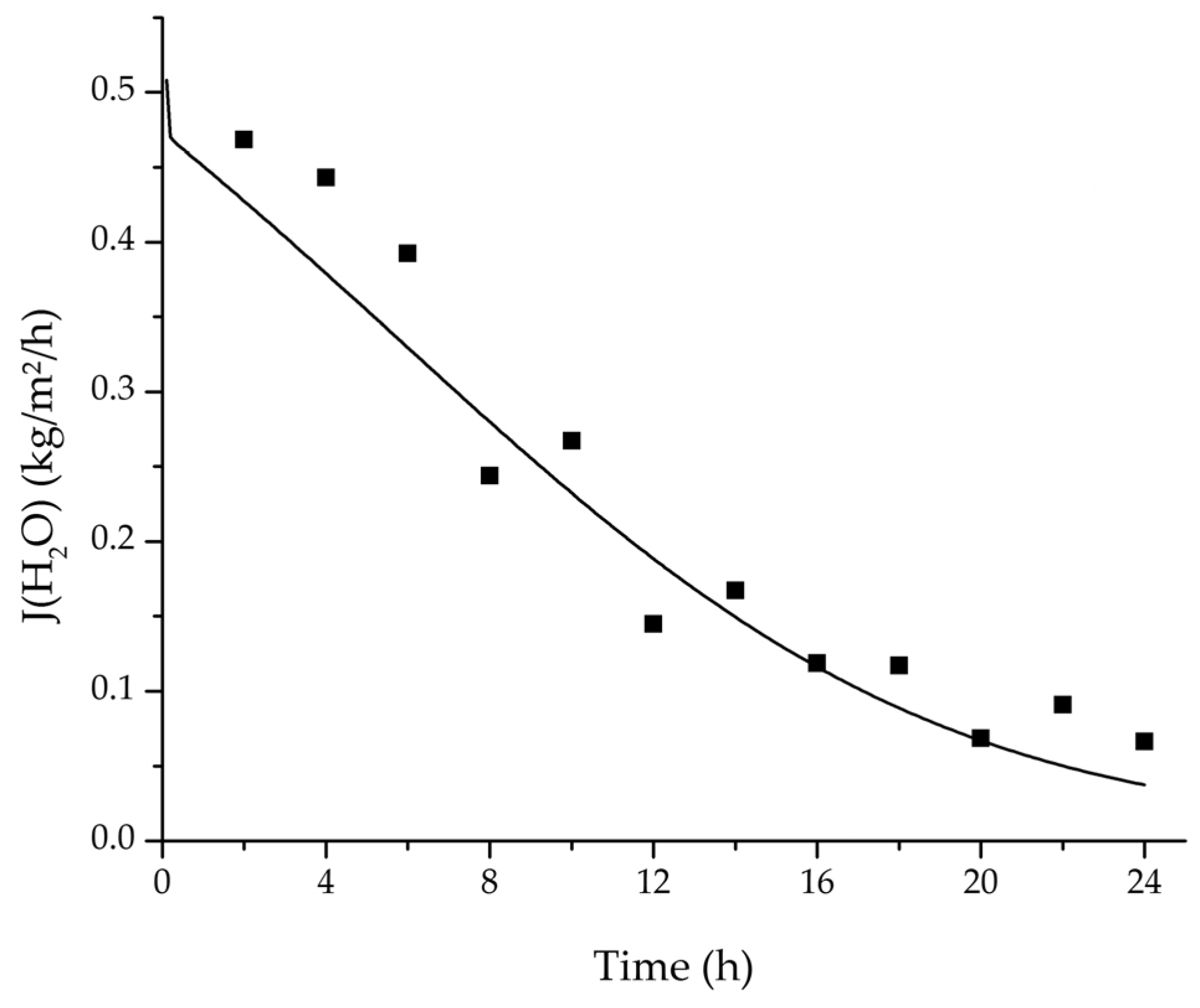
Figure 16.
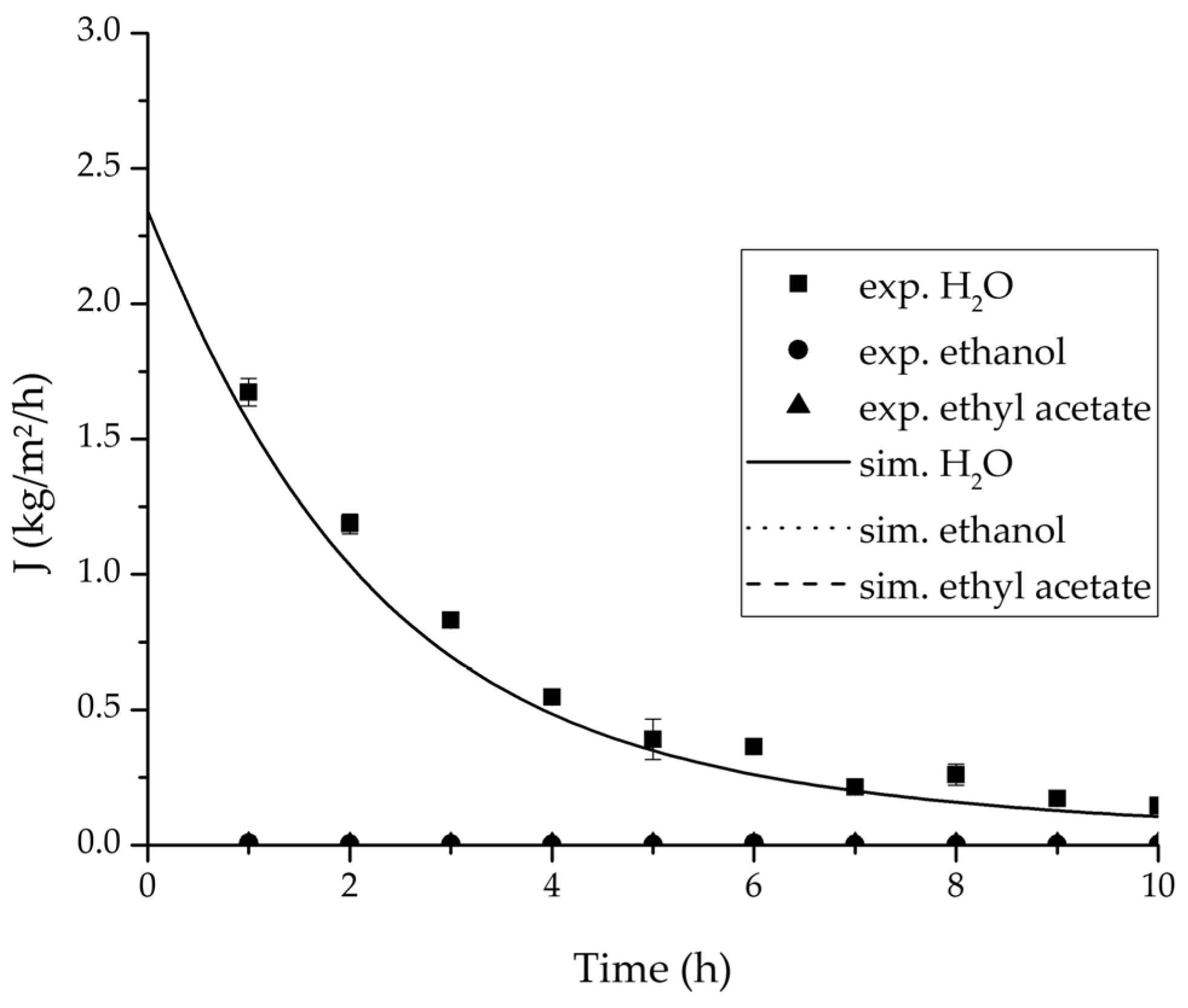
Experimental and simulation permeate fluxes for the ternary system at 95 °C feed temperature.
Figure 16.
Experimental and simulation permeate fluxes for the ternary system at 95 °C feed temperature.
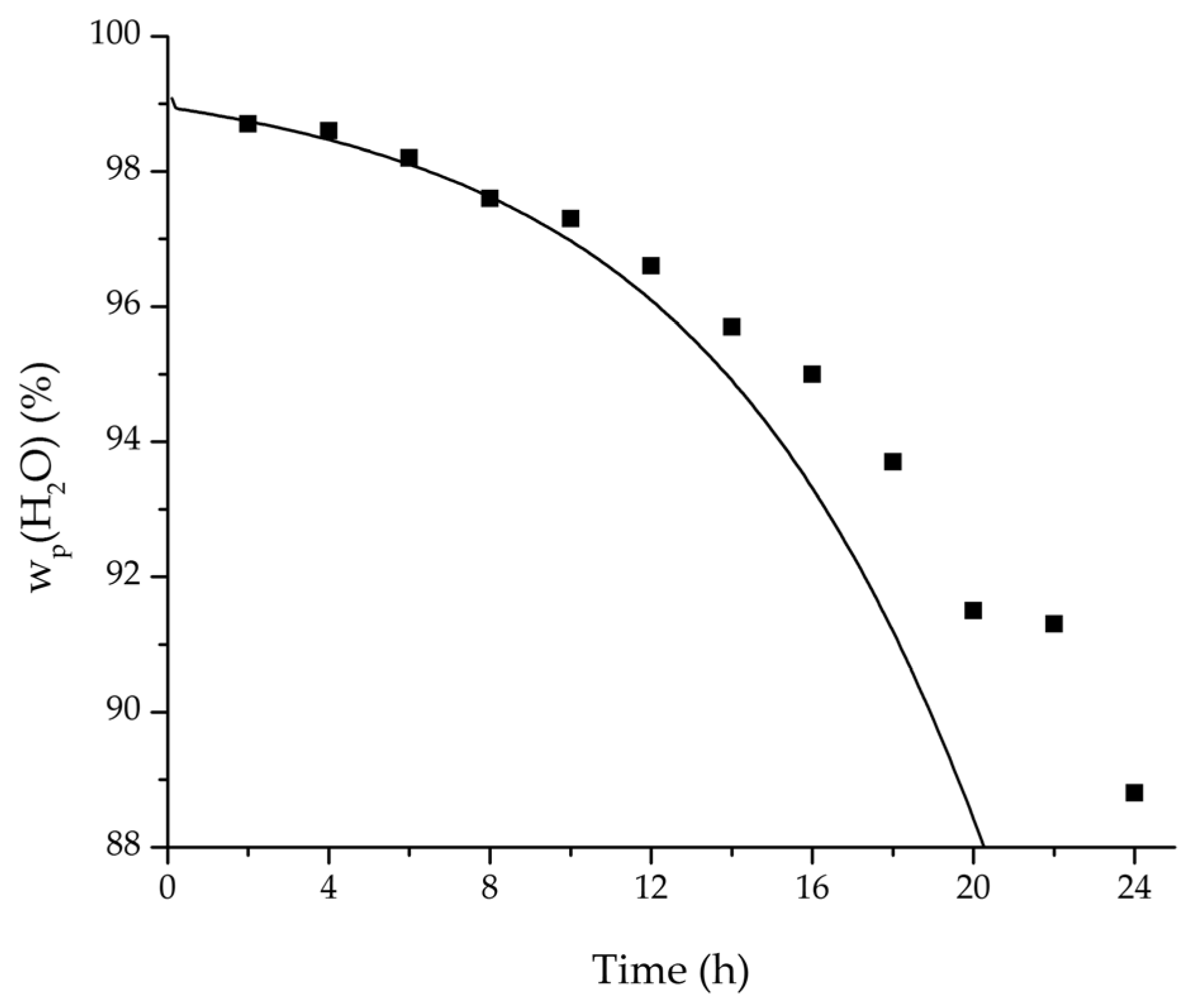
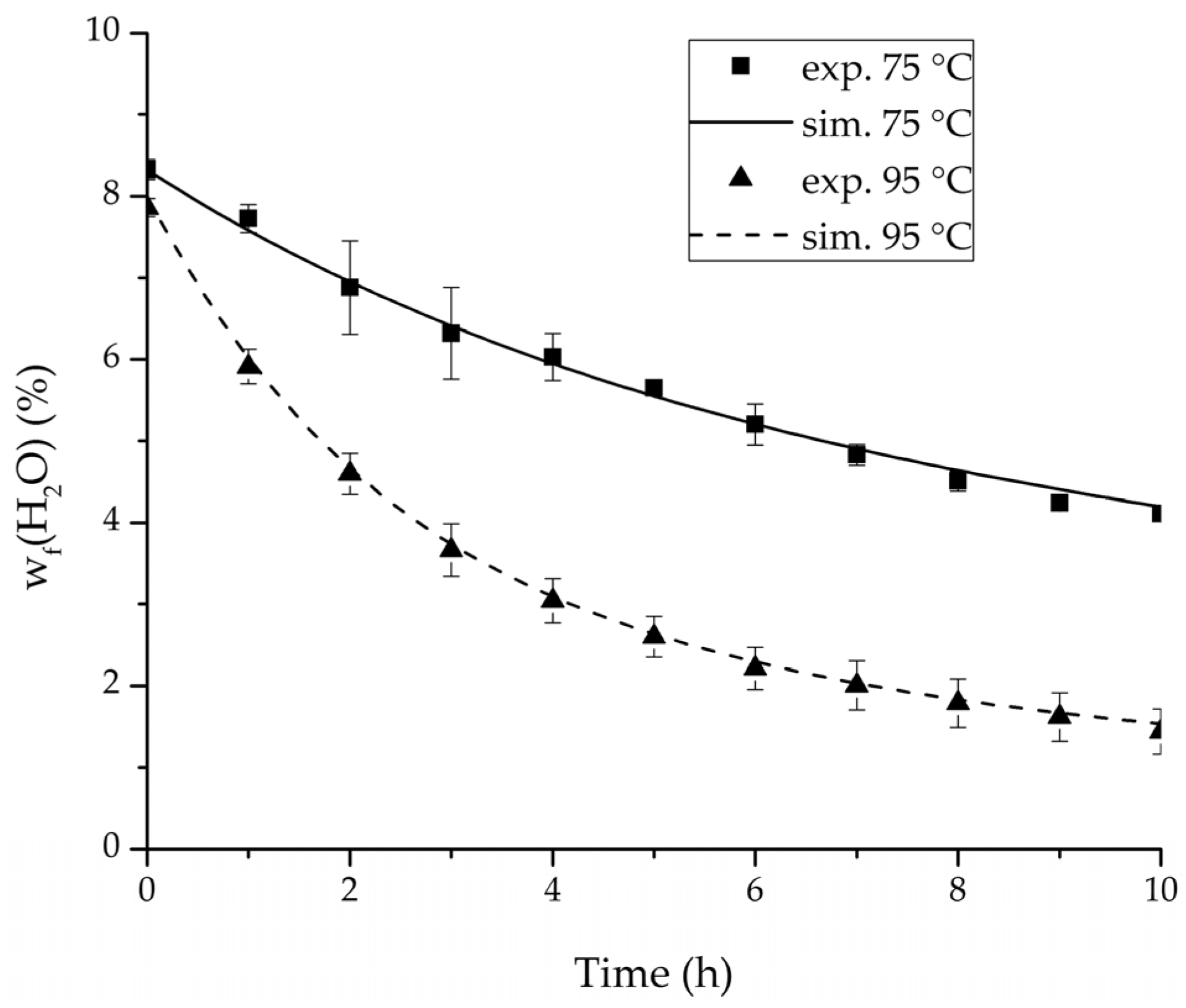
Figure 17.
Comparison of the feed water content for the ternary system at 75 °C and 95 °C feed temperature.
Figure 17.
Comparison of the feed water content for the ternary system at 75 °C and 95 °C feed temperature.
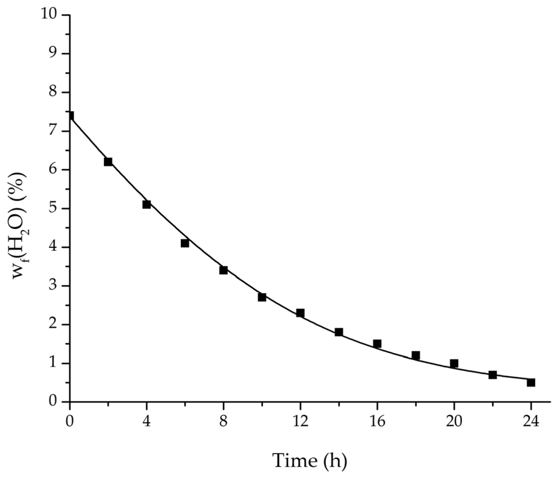
Figure 18.
Comparison of the measured and simulated water mass fraction (feed) for the pervaporation plant.
Figure 18.
Comparison of the measured and simulated water mass fraction (feed) for the pervaporation plant.
Figure 19.
Comparison of the measured and simulated water mass fraction (permeate) for the pervaporation plant.
Figure 19.
Comparison of the measured and simulated water mass fraction (permeate) for the pervaporation plant.
Figure 20.
Comparison of the measured and simulated water flux for the pervaporation plant.
Figure 20.
Comparison of the measured and simulated water flux for the pervaporation plant.
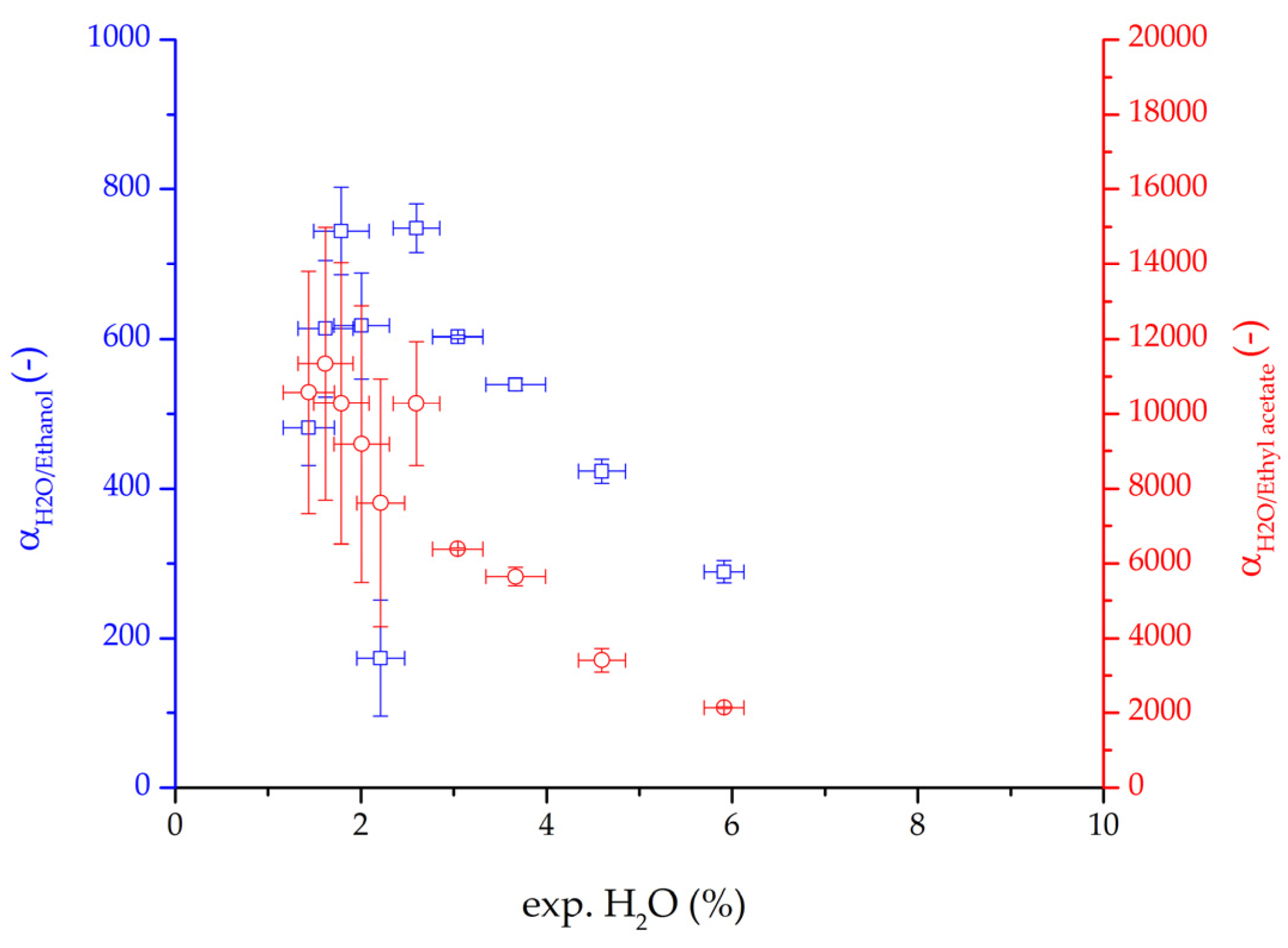
Figure 21.
Binary water/ethanol selectivity (blue squares) and water/ethyl acetate selectivity (red circles plotted over the water mass fraction (feed) for the ternary system. The error bars represent the standard deviation.
Figure 21.
Binary water/ethanol selectivity (blue squares) and water/ethyl acetate selectivity (red circles plotted over the water mass fraction (feed) for the ternary system. The error bars represent the standard deviation.
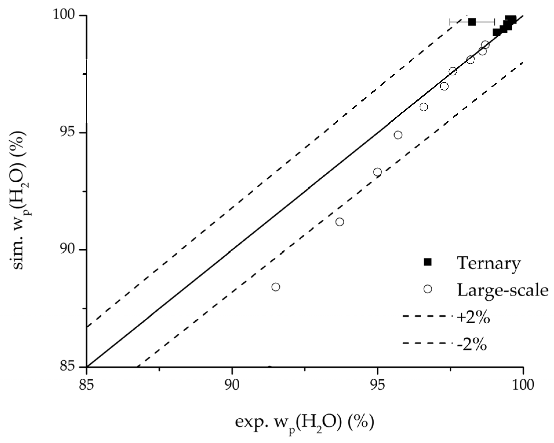
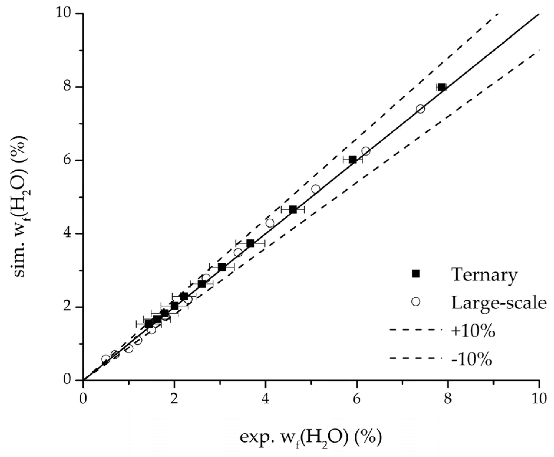
Figure 22.
Parity plot between the experimental and simulated water mass fraction (feed) for the ternary system at 95 °C feed temperature.
Figure 22.
Parity plot between the experimental and simulated water mass fraction (feed) for the ternary system at 95 °C feed temperature.
Figure 23.
Parity plot between the experimental and simulated water mass fraction (permeate) for the ternary system at 95 °C feed temperature.
Figure 23.
Parity plot between the experimental and simulated water mass fraction (permeate) for the ternary system at 95 °C feed temperature.
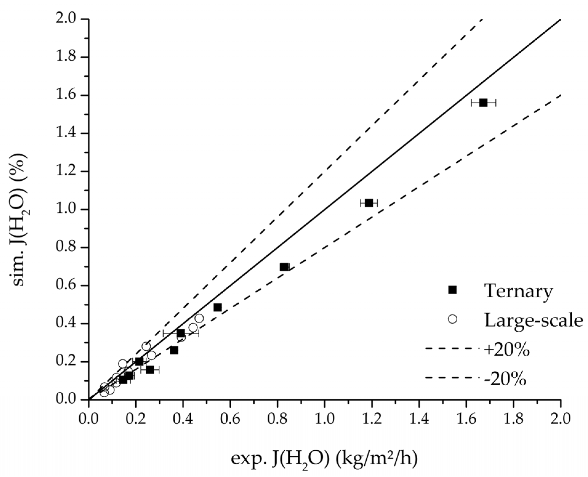
Figure 24.
Parity plot between the experimental and simulated water flux for the ternary system at 95 °C feed temperature.
Figure 24.
Parity plot between the experimental and simulated water flux for the ternary system at 95 °C feed temperature.
Table 1.
Parameter sets for Sherwood and Nusselt correlations [
21].
Table 1.
Parameter sets for Sherwood and Nusselt correlations [
21].
| Flow Regime | | | | |
|---|
| Laminar (Re < 2300) | 1.615 | 0.33 | 0.33 | 0.33 |
| Turbulent (Re > 2300) | 0.026 | 0.80 | 0.30 | 0 |
Table 2.
Experimental design for the binary system ethanol/water. Indicated (*) experiments represent the centre point experiments. Bold highlighted experiments were used for the determination of the permeance, the rest for the validation of the model. All experiments were conducted with feed pressure of 3.5 bar.
| Exp. | (%) | (°C) | (mbar) | (L/h) | (%) |
|---|
| 1 | 84.6 | 55 | 10 | 40 | 84.8 |
| 2 | 85.3 | 75 | 100 | 70 | 87.4 |
| 3 | 85.2 | 95 | 10 | 70 | 96.4 |
| 4 | 86.2 | 95 | 100 | 40 | 94.6 |
| 5 * | 90.1 | 85 | 55 | 55 | 93.8 |
| 6 * | 90.0 | 85 | 55 | 55 | 94.5 |
| 7 * | 90.3 | 85 | 55 | 55 | 94.7 |
| 8 | 94.9 | 75 | 10 | 70 | 96.6 |
| 9 | 95.0 | 75 | 100 | 40 | 95.3 |
| 10 | 95.4 | 95 | 10 | 40 | 98.6 |
| 11 | 95.2 | 95 | 100 | 70 | 97.1 |
Table 3.
Experimental design for the binary system ethyl acetate/water. Indicated (*) experiments represent the centre point experiments. Bold highlighted experiments were used for the determination of the permeance, the rest for the validation of the model. All experiments were conducted with feed pressure of 3.5 bar.
| Exp. | (%) | (°C) | (mbar) | (L/h) | (%) |
|---|
| 1 | 97.1 | 50 | 10 | 40 | 98.2 |
| 2 | 97.2 | 50 | 100 | 70 | 97.3 |
| 3 | 96.6 | 70 | 10 | 70 | 97.8 |
| 4 | 97.0 | 70 | 100 | 40 | 98.4 |
| 5 * | 97.2 | 60 | 55 | 55 | 97.6 |
| 6 * | 98.1 | 60 | 55 | 55 | 98.7 |
| 7 * | 97.9 | 60 | 55 | 55 | 98.4 |
| 8 | 99.1 | 70 | 10 | 40 | 99.1 |
| 9 | 92.3 | 95 | 10 | 40 | 99.1 |
| 10 | 93.9 | 95 | 100 | 70 | 99.0 |
| 11 | 92.5 | 70 | 100 | 40 | 98.2 |
| 12 | 91.7 | 70 | 10 | 70 | 98.0 |
Table 4.
Overview of process parameters used in the ternary experiments. The mass fractions are given for the start of the experiments and in brackets after 10 h. The mass fractions listed are the mean value based on the thrice-repeated experiments. All experiments were conducted with a feed pressure of 5 bar.
| Exp. | (%) | (%) | (%) | (°C) | (mbar) | (L h−1) |
|---|
| 1 | 16.0 (16.4) | 76.1 (81.3) | 7.9 (1.4) | 95 | 54 | 70 |
| 2 | 16.0 (17.1) | 75.7 (78.1) | 8.3 (4.1) | 75 | 54 | 70 |
Table 5.
Process parameters and ethanol mass fraction after 24 h for the industrial pervaporation plant. 15,000 kg of ethanol/water solution were dehydrated, resulting in a total permeate mass of 1070 kg.
Table 5.
Process parameters and ethanol mass fraction after 24 h for the industrial pervaporation plant. 15,000 kg of ethanol/water solution were dehydrated, resulting in a total permeate mass of 1070 kg.
| (%) | (°C) | (bar) | (mbar) | (L h−1) | (%) |
|---|
| 92.6 | 95 | 6.35 | 15 | 8000 | 99.1 |
Table 6.
Determined permeance data for the two binary systems by a nonlinear least squares regression, minimizing the weighted square error between experiments and simulation. For the simulation of the ternary system, the organic solvent permeance data was adopted from the binary data. The water permeance data for the ternary simulation was adopted from the ethyl acetate/water data.
| Exp. | Component | | | | Equation |
|---|
| binary | ethanol | 0.02 | 0 | 5 | (25) |
| water | 2.3 | 0 | 3 | (25) |
| binary | ethyl acetate | 0.01 | 0 | 3.1 | (26) |
| water | 361.1 | 0 | 3.4 | (26) |
| ternary | ethanol | 0.02 | 0 | 5 | (25) |
| ethyl acetate | 0.01 | 0 | 3.1 | (26) |
| water | 361.1 | 0 | 3.4 | (26) |


