
The Airflow Field Characteristics of UAV Flight in a Greenhouse
by
Qiang Shi
1,2, 
Yulei Pan
1,2, 
Beibei He
1,2,
Huaiqun Zhu
1,2,
Da Liu
1,2,
Baoguo Shen
1,2 and
Hanping Mao
1,2,* 1
Key Laboratory of Modern Agricultural Equipment and Technology, Ministry of Education of the People’s Republic of China, Jiangsu University, Zhenjiang 212013, China
2
High-Tech Key Laboratory of Agricultural Equipment and Intelligence of Jiangsu Province, Zhenjiang 212013, China
*
Author to whom correspondence should be addressed.
Agriculture 2021, 11(7), 634; https://doi.org/10.3390/agriculture11070634
Submission received: 21 June 2021
/
Revised: 6 July 2021
/
Accepted: 6 July 2021
/
Published: 7 July 2021
Abstract
:The downwash airflow field of UAVs is insufficient under the dual influence of greenhouse structure and crop occlusion, and the distribution characteristics of the flight flow field of UAVs in greenhouses are unclear. In order to promote the application of UAVs in greenhouses, the flow field characteristics of UAVs in a greenhouse were studied herein. In a greenhouse containing tomato plants, a porous media model was used to simulate the obstacle effect of crops on the airflow. The multi-reference system model method was selected to solve the flow field of the UAV. Studies have shown that the airflow field generated by UAV flight in a greenhouse is mainly affected by the greenhouse structure. With the increase in UAV flight height, the ground effect of the downwash flow field weakened, and the flow field spread downward and around. The area affected by the flow field of the crops became larger, while the development of the crop convection field was less affected. The simulation was verified by experiments, and linear regression analysis was carried out between the experimental value and the simulation value. The experimental results were found to be in good agreement with the simulation results.
1. Introduction
Unmanned aerial vehicles (UAVs) offer a highly efficient and nondestructive method for spraying pesticides on crops and have been widely used in the agricultural industry, representing advanced agricultural technology [1,2,3]. Since agricultural UAVs are usually constructed of light materials with low stiffness, various airflows have a great impact on the stability, safety, and pesticide application of UAV flight [4,5,6], ultimately increasing the operation error. In order to improve the accuracy of UAV operation, it is necessary to study the characteristics of the UAV flow field, especially the downwash flow field.
In recent years, studies have shown that the airflow field of UAVs is generated downward from the rotor [7], as the maximum velocity field is maintained below the rotor [8], and its strength can be changed by adjusting the flight altitude [9]. Ni et al. [10] simulated the airflow field of different UAV flight altitudes using computational fluid dynamics (CFD) simulation software, which confirmed that the increase in UAV flight altitude will increase the area of the airflow field, but the velocity of the airflow field will decrease. At the same height, the farther away from the center of the flow field, the smaller the airflow velocity and velocity gradient. This is the conclusion when the UAV is still. Zhang et al. [11] successfully established a three-dimensional airflow field model of a six-rotor plant protection UAV using LBM (Lattice Boltzmann Method, LBM) and provided the UAV flight speed. The experiment showed that when the flight altitude was 3 m, the flight speed increased, and the airflow tilted obviously backward. At 1 m/s, due to the small velocity, the airflow diffused on the ground to produce a vortex ring and further moved backward. When the flight speed was above 2 m/s, the vortex ring disappeared, producing a Λ-shape transverse separation flow. When the velocity reached 4 m/s, the wake separated from the ground and formed a horseshoe vortex, which indicated that the velocity was no longer suitable for agricultural application. Li et al. [12] collected, analyzed, and processed experimental data from drone pollinators in the field and constructed a one-way two-dimensional wind field model of a drone rotor at the rice canopy using Fourier fitting, Gaussian fitting, and polynomial fitting. It was found that an important “steep wall” effect was observed when the wind speed under the drone rotor reached its maximum value, and the increased rate of forward wind speed was significantly higher than that of backward reduction. The whole wind field “steep wall” was symmetrical along the UAV flight direction. Wang et al. [13] analyzed from the perspective of the number of UAV rotors and measured the wind speed of rotor airflow perpendicular to the flight direction X, perpendicular to the ground direction Y, and parallel to the flight direction Z using a wind field sensor network measurement system under three types of UAV flight operation conditions. The experimental results showed that the wind power of a single rotor and four-rotor UAV in the downwash flow field perpendicular to the flight direction was the largest, while the wind power of the eight-rotor UAV in the vertical direction was the largest, which demonstrated the reason for the best application effect of an eight-rotor UAV. Guo et al. [14] combined compressible Reynolds-averaged Navier–Stokes (RANS) equations, the shear stress transport (SST) k-ω turbulence model, sliding grid technology and the Semi-Implicit Method for Pressure Linked Equations (SIMPLE) algorithm to establish the computational fluid dynamics model of the downwash flow of a four-rotor agricultural UAV during hovering. The downwash flow field of the UAV was divided into four regions from time dimension analysis. It was found that the z-direction velocity of the downwash flow field differed with height, and the speed of stabilization also differed but stabilized in about 4 s. After the downwash flow field was stable, with the decrease in height, the influence of the rotor was weakened, and the airflow velocity right below the rotor was also reduced. However, due to atmospheric compression and airflow induction, the downwash velocity in the other three regions increased with decreasing height. In addition, at the same time and at the same height, the downwash velocity right below the rotor was greater than the other three regions. In another study, Li et al. [15] used an S-shaped pitot array and installed wind speed sensors to obtain wind field data. Vertical data, such as equivalent area, wind field width, and attenuation rate, were analyzed. It was found that when the plant distribution and density characteristics of rice were consistent, the lower the height, the smaller the wind field and the greater the decrease. That is, the dense leaves in the lower part significantly hindered the airflow, and the permeability of the wind field decreased with the decrease in height. Li et al. also analyzed the abnormal data in the range of 6.5 m/s (Pmedium) and 3.5 m/s (Pbottom) and found that this was caused by the vortex formed by the interaction between the wind field and the rice canopy. Finally, the ideal cone model was established based on the attenuation rate of the equivalent area of the rotor area and the equal height. Shi et al. [16] studied the wind-induced response of rice under the action of a multi-rotor UAV downwash flow field by using turbulence intensity and maximum wind speed as parameters. It was found that the downwash flow field was less affected by the external environment at low flight altitude, the pulsation characteristics were not obvious, and the turbulence intensity was not high. When the flight altitude was greater than 3 m, the turbulence intensity increased significantly with the increase in flight altitude. It is considered that the friction between the downwash flow field and the external low-speed air produces many different sizes of eddy currents during long-distance transmission. The eddy current system leads to a decrease in the downwash flow field velocity, an irregular change in the flow direction, and an increase in the turbulence intensity. With the increase of UAV flight height, the turbulence intensity at the rice canopy peaked and then gradually decreased to the final value consistent with the turbulence intensity of the ambient wind, but it was still much larger than that of the ambient wind conditions.
In summary, the research on UAV flow fields has mainly focused on the flow field under different flight conditions in outdoor environments and the blocking effect of crop convection field. There is still a lack of research on the characteristics of the UAV airflow field within a greenhouse structure. Therefore, in this study, a greenhouse planted with tomato was used as the research environment, and the CFD method was used to obtain the flow field simulation results of the UAV under different flight states in the greenhouse. The flow field distribution law of the UAV in the greenhouse was analyzed, and the accuracy of the simulation results was verified experimentally. These findings provide a theoretical reference for the application of UAVs in greenhouse plant protection.
2. Materials and Methods
2.1. Establishment of the Simulation Model
The three-dimensional model of the UAV was established based on the E360-S2 UAV of CNOOC. The main parameters are shown in Table 1. The rotor 8045 was obtained by an EXAscan handheld three-dimensional laser scanner. In order to facilitate grid division and simulation convergence, the UAV frame was simplified. The UAV model is shown in Figure 1.
Taking the cuboid of 17 m × 0.8 m × 1.2 m as the crop model, the crop was treated by the porous medium model to simulate the blocking effect of crops on airflow. The porous media model is based on Darcy–Forchheimer law and expressed as
where S is the momentum loss term; μ is the dynamic viscosity, N·s/m2; α is permeability, 0.395 m2 [17]; ρ is fluid density, 1.225 kg/m3; and C2 is the inertia loss coefficient, 0.4 [17]. According to a Venlo greenhouse, a three-dimensional model was established. Its parameters are shown in Table 2. The established greenhouse model is shown in Figure 2. The diagram simplifies the structure of air exchange inside and outside the greenhouse and only depicts its geometric structure.
The three-dimensional model was assembled to obtain the greenhouse-crop-UAV model, as shown in Figure 3. The greenhouse contained a tomato crop with an average height of approximately 2 m during the period of measurement and a leaf area index of about 1.5 m2 leaf per m2 ground. The height and leaf area of tomato were slightly lower than that of Molina-Aiz [18].
2.2. Grid Division
ICEM-CFD was used to mesh the model. The greenhouse volume was over 1000 m3, and the maximum unit size was set to 0.3 m. The size of the UAV was small, and the grid division of the rotor had a great influence on the simulation results of the flow field. The grid of the UAV was encrypted, and the maximum unit size of the rotor was set to 0.0005 m. The grid model is shown in Figure 4. Number of rotor grids is shown in Table 3.
2.3. Solution Settings
The total calculation domain was within the whole greenhouse structure. In order to ensure the solution accuracy of the numerical simulation, the calculation domain was divided into four rotation domains (set the rotation speed of 6000 rpm), porous media area, cultivation groove solid area, and air area in the greenhouse. Rotation calculation domain is shown in Figure 5. The interface between rotation and air area was connected by interface.
Since the k-ω SST model can better predict the flow and swirl in the near-wall region in the simulation of the external flow field, the k-ω SST turbulence model was set up. The SIMPLE algorithm was used for the coupling of pressure and velocity, and the multi-reference system model method was used to solve the flow field of the UAV.
In order to simulate the actual operation situation of the UAV to study the influence of flight height, inter-row position, and crop conditions (whether there are any crops) in the greenhouse on the airflow field of a UAV in the greenhouse, an orthogonal experiment (Table 4) was designed to simulate the flow field. Flgiht position layout of UAV in greenhouse is shown in Figure 6.
3. Results
3.1. Effect of Flow Field on Crops
After the 1.5 m east–west development of the UAV downwash flow field, the wind speed tended towards zero. It can be seen from Figure 7 that the crop areas on both sides of the UAV were affected by the flow field of the UAV. The maximum wind speed in the crop canopy area was 2.8 m/s, which is not conducive to the image data acquisition of crops by UAVs.
3.2. Effects of Crops on the Flow Field
In this study, a greenhouse with tomatoes was used to obtain the wind speed on both sides of the tomato crop near the UAV. The results are shown in Figure 8. The two velocity curves of the crops on the far side of the UAV were approximately coincident, and the maximum velocity difference was 0.07 m/s. By contrast, the wind velocity curves of the crops near the UAV were quite different, particularly in the range of 0.35–1.1 m away from the ground, where the two curves were obviously not coincident. In the vicinity of the crops, the flow field near the UAV side was not fully developed, and the wind speed was slightly lower. The maximum velocity difference between the two was 0.36 m/s. In general, tomato plants have a small leaf area and low leaf density, which have no obvious effect on airflow blocking.
3.3. Effect of Greenhouse Structure on Flow Field
The UAV was limited by the height of the greenhouse, and so the flight height was generally less than 3 m. There was an obvious ground effect, and a near-surface regional flow field developed on the wall on both the north and south sides of the greenhouse. Occluded by the cultivation trough, the flow field extended 1.5 m in the east–west direction (Y-Z plan)and then decreased to 0 m/s, and the development area was far less than the north–south (X–Y plane) flow field, as shown in Figure 9. The cultivation tank was the main factor restricting the development of the UAV flow field.
3.4. Effect of Flight State on Flow Field
Figure 10 shows the flow field distribution of the X–Y plane and the crop near the UAV side when the UAV is in the middle of flight. From top to bottom, the flight height increased continuously. The downwash flow field of the UAV developed more fully downward and around, and the ground effect weakened, while the impact on crops increased. As shown in Figure 11, the affected area of the crops doubled with the increase in flight height by 40 cm.
According to the 3D velocity volume data, all the velocity volume details were displayed on the 2D image at the same time, which was called velocity volume rendering. The velocity volume rendering was used to display the comprehensive distribution of the airflow field in the two-dimensional image, and through the control of the opacity, the situation of the velocity isosurface was reflected. Figure 11 shows a speed volume rendering of four locations in the middle of the row, in the quarter of the row, at the end of the row, and in the aisle. It can be seen that the flow field mainly developed between the rows when the UAV hovered. When the UAV hover position gradually moved to the northern side of the greenhouse, the symmetry of the flow field distribution in the greenhouse disappeared, and the wind speed in the northern side of the greenhouse increased, resulting in a larger wind speed on the side of the UAV flight altitude, which affected the flight state of the UAV and caused a decrease in flight stability.
4. Test Validation
The UAV was suspended at 1.5 m height and had a midline position. The wind speed at 0.3 m, 0.6 m, and 0.9 m height was measured by a KIMO VT110 anemometer. Greenhouse test is shown in Figure 12. The test and simulation results are shown in Table 5.
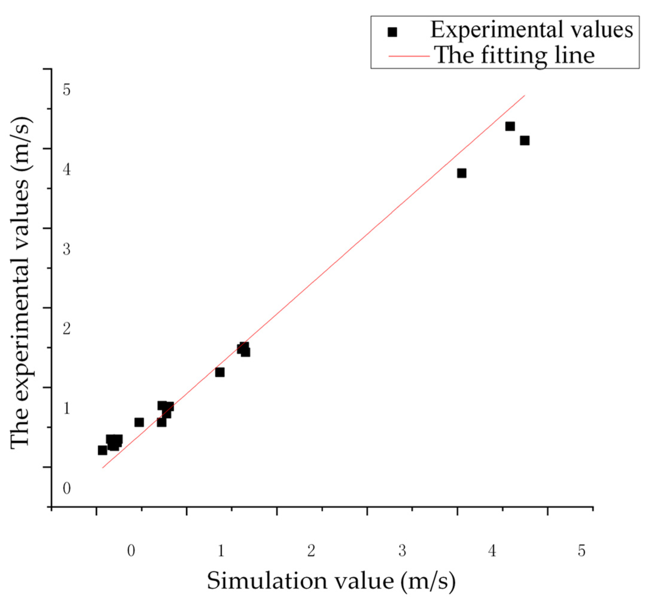
Linear regression analysis was performed on the experimental and simulated values (Figure 13). The regression fitting equation was y = x − 0.08139, the R2 was 0.97486, and the significance level was 0.05. In summary, the numerical simulation results of the UAV greenhouse airflow field were accurate.
5. Conclusions
During the flight of the four-rotor UAV in the greenhouse, the flow field was mainly hindered by the cultivation groove, and the flow field was not fully developed. The flow field was mainly concentrated at the bottom of the crop and the junction of the cultivation groove, and the flow field only affected the adjacent crops. Tomatoes have a small leaf area and low leaf density and thus had little effect on the flight flow field of the UAV in the greenhouse.
When the UAV flight height increased, the flow field developed more fully downward and around, and the affected area of the crops became larger. For every 40-cm increase in flight height, the affected area doubled. When the UAV moved to one side between rows, the flow field distribution in the greenhouse was asymmetric, and the flight stability decreased.
Through the experimental verification, linear regression analysis was carried out on the measured value and the simulated value, and the goodness of fit (R2) was 0.97486, which verified the accuracy of the simulation results of the airflow field of the UAV in the greenhouse.
6. Limitations
This study did not consider the coupling effect of window ventilation and UAV downwash flow field. According to Espinoza et al.’s [19] research, window ventilation could significantly change the microclimate in greenhouse. Mostly, the air flow of the window ventilation is much larger than that of the UAV downwash flow field, for the whole greenhouse. When the window ventilation and the UAV downwash flow field worked together, the window ventilation factor may occupy the dominant position. However, due to the large local wind speed of the UAV downwash flow field, the downwash flow field may occupy the dominant position near the UAV.
It is necessary to further study and analyze the change law of greenhouse microclimate under the competitive coupling of window ventilation and UAV downwash flow field.
Author Contributions
Conceptualization, Q.S. and H.M.; methodology, Q.S.; software, Q.S. and Y.P.; validation, H.Z. and D.L.; formal analysis, B.H.; investigation, B.S.; resources, Q.S.; data curation, H.Z. and Q.S.; writing—original draft preparation, H.Z.; writing—review and editing, Q.S. and Y.P.; visualization, Q.S.; supervision, H.M.; project administration, Q.S.; funding acquisition, H.M. All authors have read and agreed to the published version of the manuscript.
Funding
This research was financially supported by the Priority Academic Program Development of Jiangsu Higher Education Institutions (PAPD-2018-87); Open Fund of the Ministry of Education Key Laboratory of Modern Agricultural Equipment and Technology & High-tech Key Laboratory of Agricultural Equipment and Intelligentization of Jiangsu Province (JNZ201907).
Institutional Review Board Statement
The study did not involve humans or animals.
Informed Consent Statement
Not applicable.
Data Availability Statement
No new data were created or analyzed in this study. Data sharing is not applicable to this article.
Conflicts of Interest
The authors declare no conflict of interest.
References
- Qin, W.; Xue, X.; Zhang, S.; Gu, W.; Wang, B. Droplet deposition and efficiency of fungicides sprayed with small UAV against wheat powdery mildew. Int. J. Agric. Biol. Eng. 2018, 11, 27–32. [Google Scholar] [CrossRef] [Green Version]
- Ahmad, F.; Qiu, B.; Dong, X.; Ma, J.; Huang, X.; Ahmed, S.; Chandio, F.A. Effect of operational parameters of UAV sprayer on spray deposition pattern in target and off-target zones during outer field weed control application. Comput. Electron. Agric. 2020, 172, 105350. [Google Scholar] [CrossRef]
- Yao, H.; Qin, R.; Chen, X. Unmanned Aerial Vehicle for Remote Sensing Applications—A Review. Remote. Sens. 2019, 11, 1443. [Google Scholar] [CrossRef] [Green Version]
- Urita, A. Aerodynamic Characteristics of Elastic Wings Morphed and Vibrated in Uniform Flows and Separated Flows Around Them. Flow Turbul. Combust. 2018, 102, 457–467. [Google Scholar] [CrossRef]
- Ren, Z.; Fu, W.; Yan, J. Gust Perturbation Alleviation Control of Small Unmanned Aerial Vehicle Based on Pressure Sensor. Int. J. Aerosp. Eng. 2018, 2018, 7259363. [Google Scholar] [CrossRef] [Green Version]
- Zhou, S.; Shen, A.; Wang, M.; Peng, S.; Liu, Z. Study on Composing Dense Formations in a Dynamic Environment of Multirotor UAVs by Distributed Control. Math. Probl. Eng. 2018, 2018, 7878094. [Google Scholar] [CrossRef]
- Brinkman, L.J.; Davis, B.; Johnson, E.C. Post-movement stabilization time for the downwash region of a 6-rotor UAV for remote gas monitoring. Heliyon 2020, 6, e04994. [Google Scholar] [CrossRef] [PubMed]
- Tang, Q.; Zhang, R.; Chen, L.; Xu, G.; Deng, W.; Ding, C.; Xu, M.; Yi, T.; Wen, Y.; Li, L. High-accuracy, high-resolution downwash flow field measurements of an unmanned helicopter for precision agriculture. Comput. Electron. Agric. 2020, 173, 105390. [Google Scholar] [CrossRef]
- Wang, C.; He, X.; Wang, X.; Wang, Z.; Wang, S.; Li, L.; Mei, S. Distribution characteristics of pesticide application droplets deposition of unmanned aerial vehicle based on testing method of deposition quality balance. Trans. Chin. Soc. Agric. Eng. 2016, 32, 89–97. [Google Scholar]
- Ni, J.; Yao, L.; Zhang, J.; Cao, W.; Zhu, Y.; Tai, X. Development of an unmanned aerial vehicle-borne crop-growth monitoring system. Sensors 2017, 17, 502. [Google Scholar] [CrossRef] [PubMed] [Green Version]
- Zhang, H.; Qi, L.; Wu, Y.; Musiu, E.M.; Cheng, Z.; Wang, P. Numerical simulation of airflow field from a six–rotor plant protection drone using lattice Boltzmann method. Biosyst. Eng. 2020, 197, 336–351. [Google Scholar] [CrossRef]
- Li, J.; Zhou, Z.; Lan, Y.; Hu, L.; Zang, Y.; Liu, A.; Zhang, T. Distribution of canopy wind field produced by rotor unmanned aerial vehicle pollination operation. Trans. Chin. Soc. Agric. Eng. 2015, 31, 77–86. [Google Scholar]
- Wang, C.; He, X.; Wang, X.; Wang, Z.; Pan, H.; He, Z. Testing method of spatial pesticide spraying deposition quality balance for unmanned aerial vehicle. Trans. Chin. Soc. Agric. Eng. 2016, 32, 54–61. [Google Scholar] [CrossRef] [Green Version]
- Guo, Q.; Zhu, Y.; Tang, Y.; Hou, C.; He, Y.; Zhuang, J.; Luo, S. CFD simulation and experimental verification of the spatial and temporal distributions of the downwash airflow of a quad-rotor agricultural UAV in hover. Comput. Electron. Agric. 2020, 172, 105343. [Google Scholar] [CrossRef]
- Li, J.; Shi, Y.; Lan, Y.; Guo, S. Vertical distribution and vortex structure of rotor wind field under the influence of rice canopy. Comput. Electron. Agric. 2019, 159, 140–146. [Google Scholar] [CrossRef]
- Shi, Q.; Liu, D.; Mao, H.; Shen, B.; Li, M. Wind-induced response of rice under the action of the downwash flow field of a multi-rotor UAV. Biosyst. Eng. 2021, 203, 60–69. [Google Scholar] [CrossRef]
- Cheng, X. Construction and Prediction of CFD Model for Spatial and Temporal Distribution of Greenhouse Environmental Factors. Ph.D. Thesis, Jiangsu University, Jiangsu, China, 2011; pp. 116–117. [Google Scholar]
- Molina-Aiz, F.; Valera, D.; Peña, A.; Gil, J.; López, A. A study of natural ventilation in an Almería-type greenhouse with insect screens by means of tri-sonic anemometry. Biosyst. Eng. 2009, 104, 224–242. [Google Scholar] [CrossRef]
- Espinoza, K.; López, A.; Valera, D.L.; Molina-Aiz, F.D.; Torres, J.A.; Pena, A. Effects of ventilator configuration on the flow pattern of a naturally-ventilated three-span Mediterranean greenhouse. Biosyst. Eng. 2017, 164, 13–30. [Google Scholar] [CrossRef]
Figure 1.
UAV model.
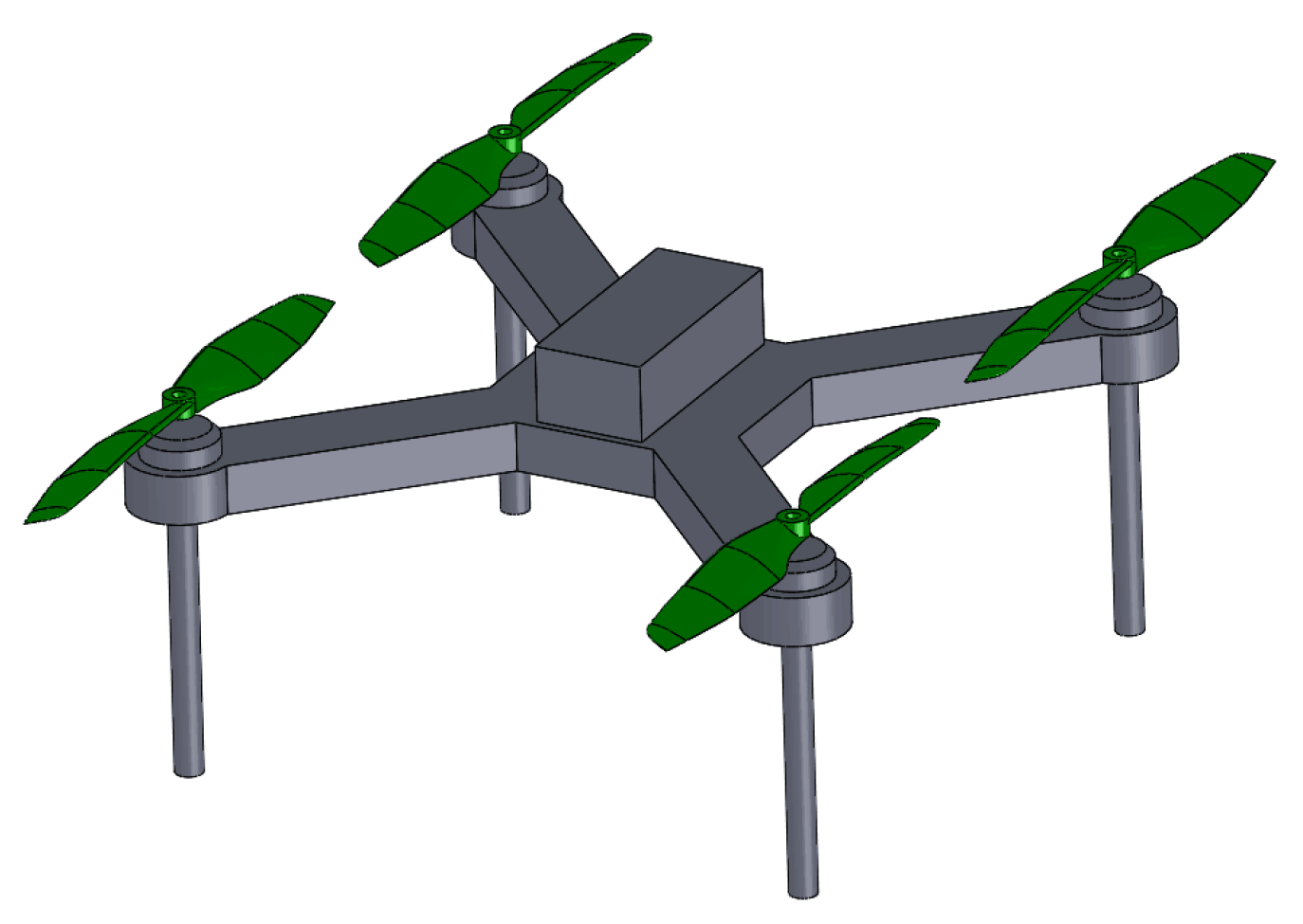
Figure 2.
Greenhouse model.

Figure 3.
Greenhouse-crop-UAV 3D model.

Figure 4.
Mesh model; (a) UAV; (b) Greenhouse.
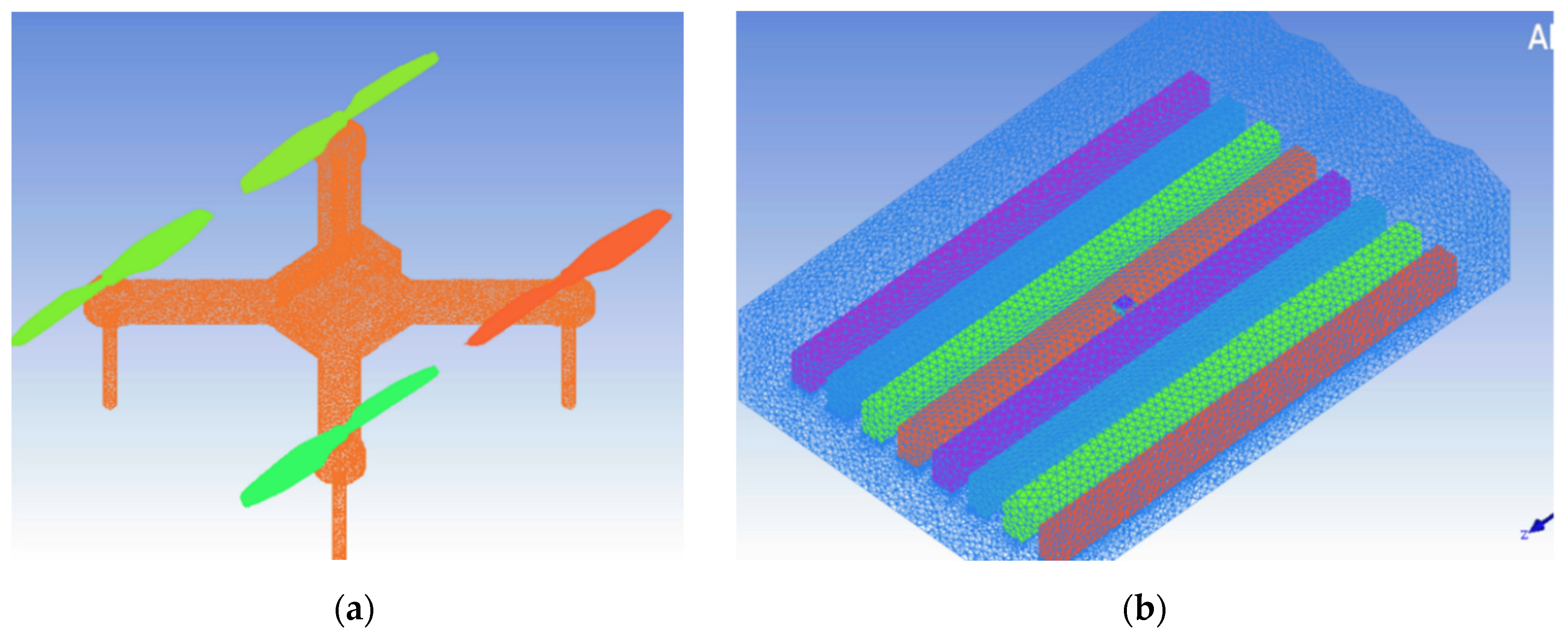
Figure 5.
Rotation calculation domain.
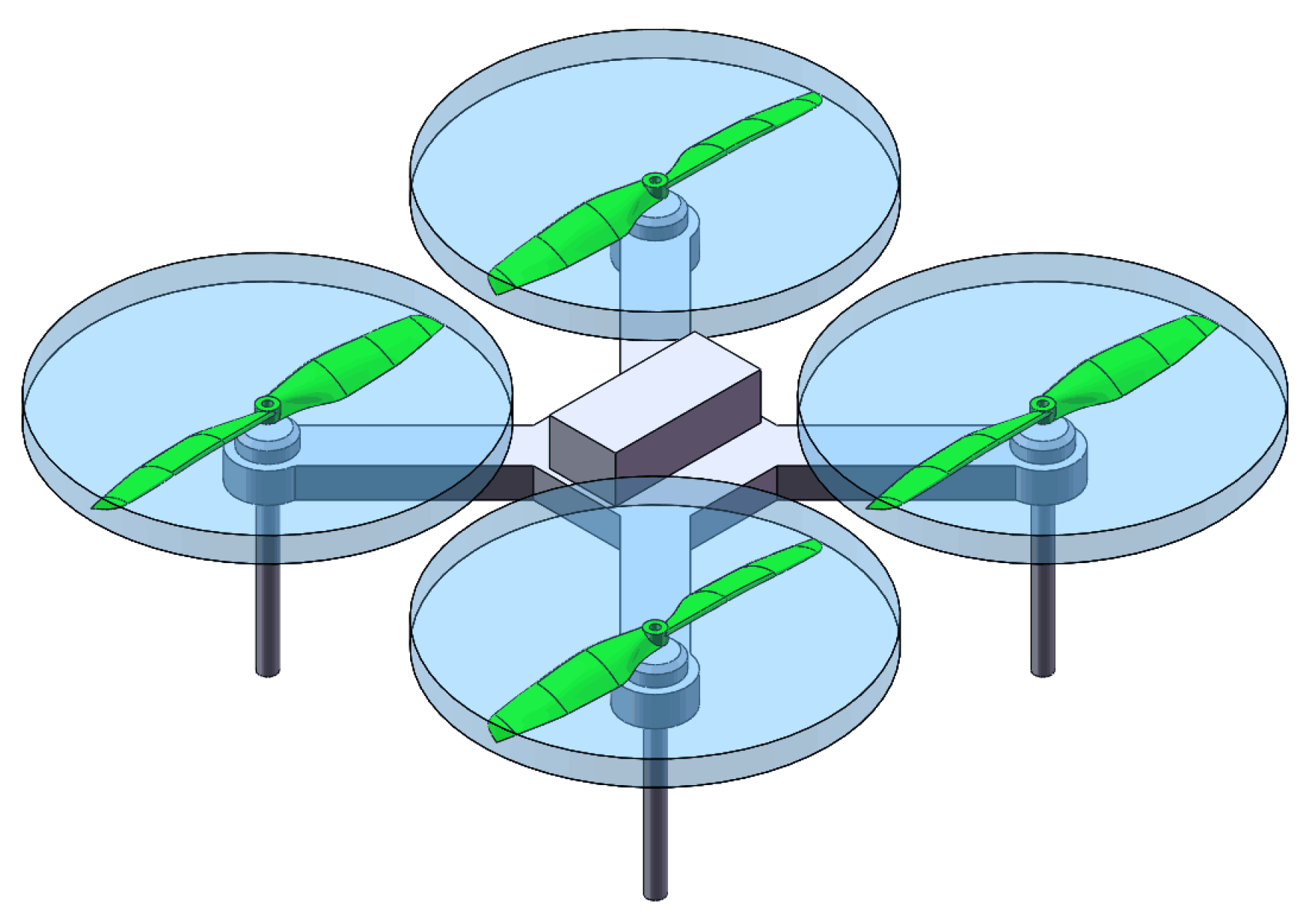
Figure 6.
Position layout of UAV. Green: crops. Red: UAV. Blue: cultivation pot. Black: greenhouse.

Figure 7.
Y–Z velocity distribution.

Figure 8.
Wind speed curves on both sides of crops.
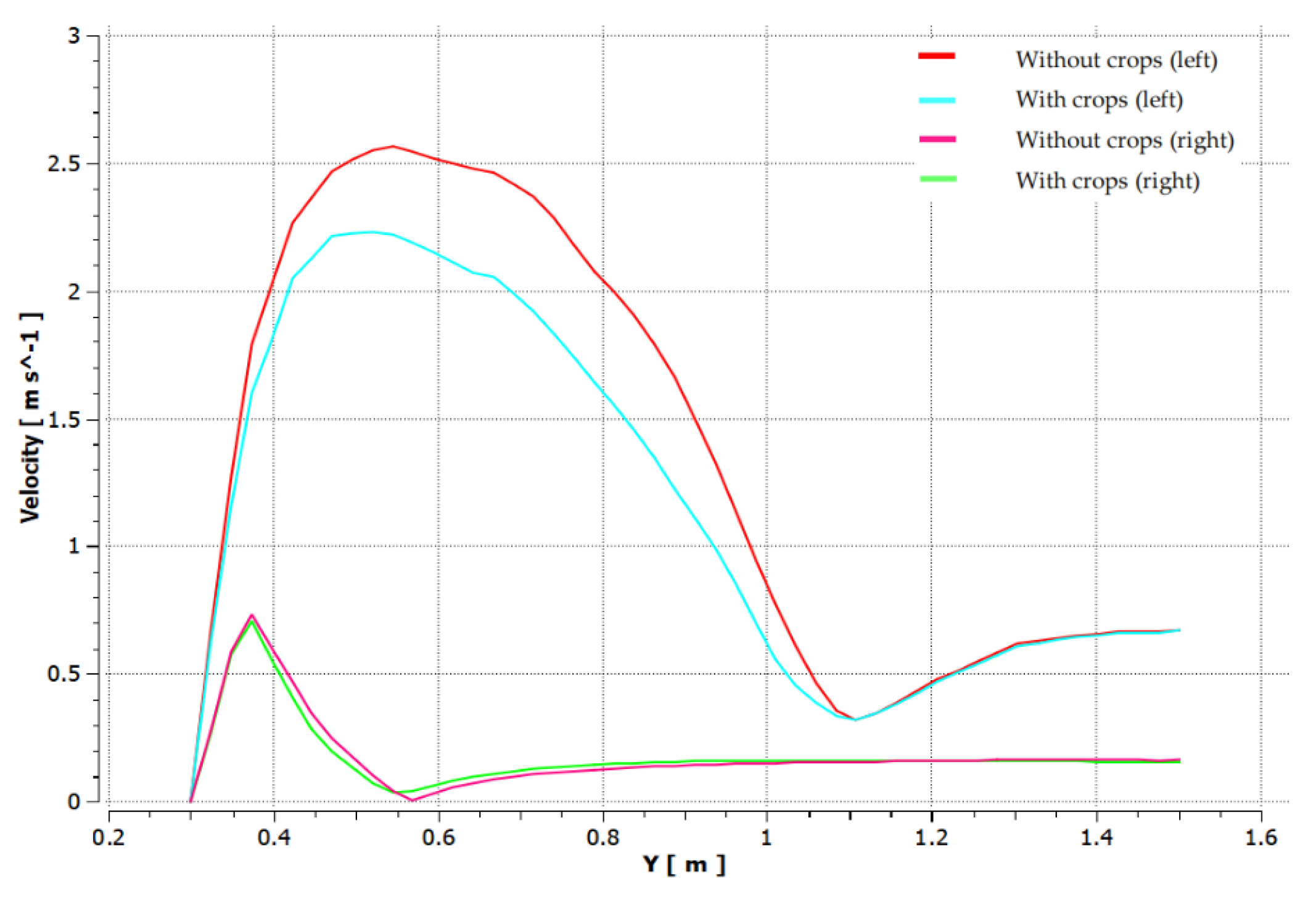
Figure 9.
Velocity distribution of the X–Y plan.
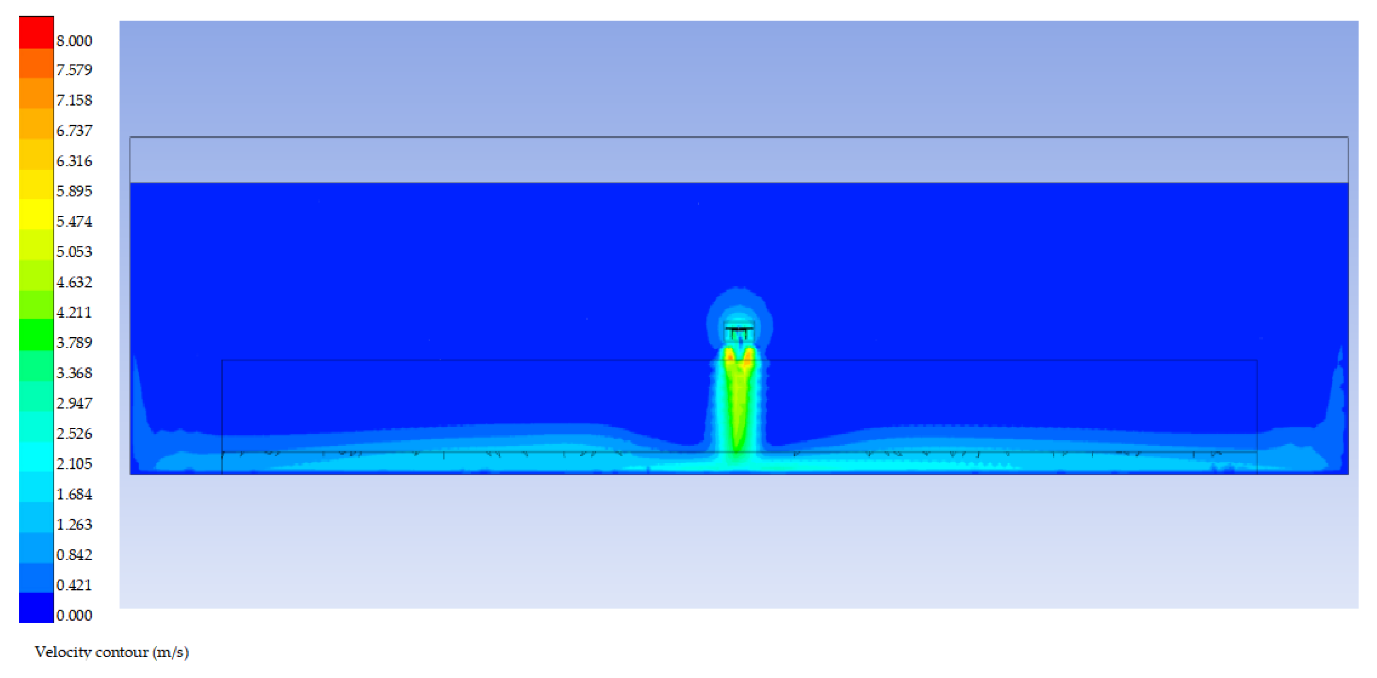
Figure 10.
Velocity contour; (a) Y = 1.1 m X–Y; (b) Y = 1.1 m crop section; (c) Y = 1.5 m X–Y; (d) Y = 1.5 m crop section; (e) Y = 1.9 m X–Y; (f) Y = 1.9 m crop section.
Figure 10.
Velocity contour; (a) Y = 1.1 m X–Y; (b) Y = 1.1 m crop section; (c) Y = 1.5 m X–Y; (d) Y = 1.5 m crop section; (e) Y = 1.9 m X–Y; (f) Y = 1.9 m crop section.
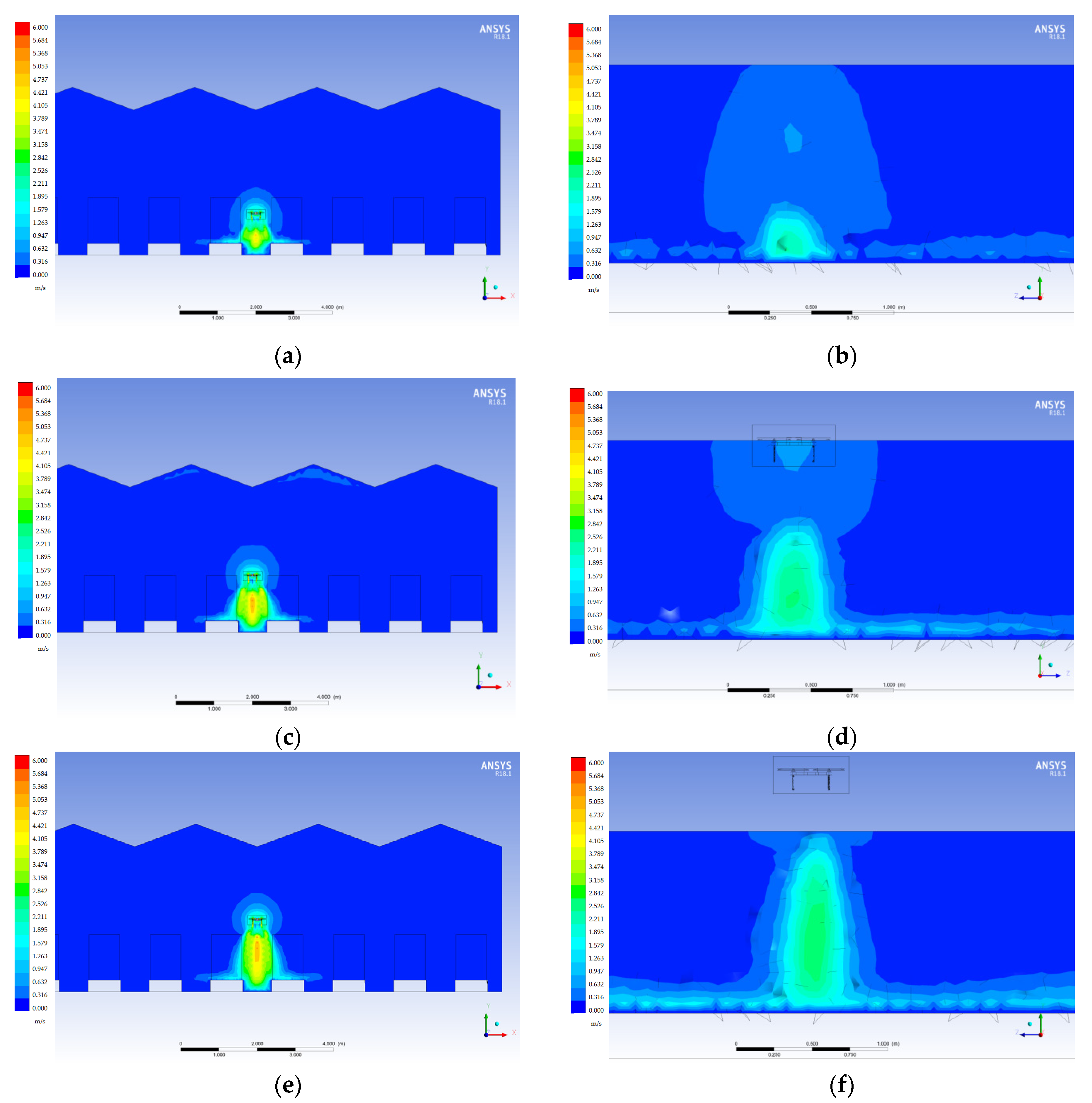
Figure 11.
Speed volume rendering. (a) In the middle of the row; (b) in the quarter of the row; (c) at the end of the row; (d) in the aisle.
Figure 11.
Speed volume rendering. (a) In the middle of the row; (b) in the quarter of the row; (c) at the end of the row; (d) in the aisle.

Figure 12.
Greenhouse test. (a) Anemometer and UAV; (b) UAV flight in greenhouse.
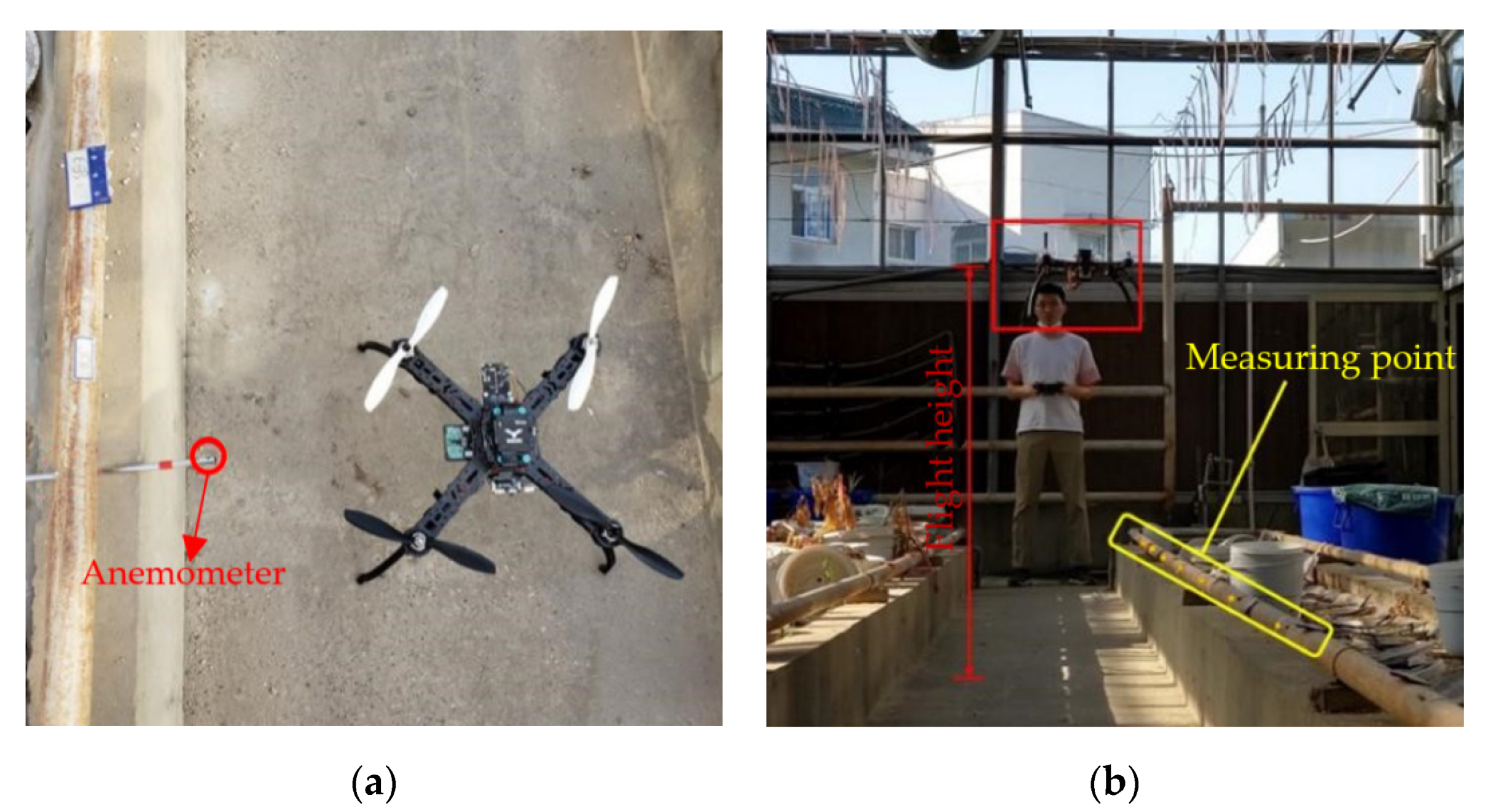
Figure 13.
Linear fitting.

Table 1.
E360-S2 UAV parameters.
| Item | Parameter |
|---|---|
| Aircraft size | 430 mm × 430 mm × 250 mm |
| Axial distance of symmetrical motor | 360 mm |
| Power motor | 2213–920 KV |
| Rotor | 8045 |
Table 2.
Venlo greenhouse parameters.
| Span | Eaves Height | Roof Height | Length | Number of Ridges |
|---|---|---|---|---|
| 3.2 m | 3.8 m | 4.4 m | 20 m | 4 |
Table 3.
Number of rotor grids.
| CCW-1 | CCW-2 | CW-1 | CW-2 |
|---|---|---|---|
| 94,896 | 95,044 | 94,952 | 94,902 |
Table 4.
Number of rotor grids.
| Test Number | Crop Conditions | Flight Height (m) | Inter-Row Position (m) |
|---|---|---|---|
| 1 | No | 1.5 | 0 |
| 2 | Have | 1.1 | 0 |
| 3 | Have | 1.5 | 0 |
| 4 | Have | 1.9 | 0 |
| 5 | Have | 1.5 | 4 |
| 6 | Have | 1.5 | 8 |
| 7 | Have | 1.5 | 9 |
Table 5.
Comparison between measured and simulated values.
| Height (m) | Distance from Midline (m) | Value of Simulation (m/s) | Experimental Value (m) | Relative Error |
|---|---|---|---|---|
| 0.3 | 0 | 4.05 | 3.69 | 0.088 |
| 1 | 0.73 | 0.77 | 0.059 | |
| 2 | 1.37 | 1.19 | 0.131 | |
| 3 | 1.65 | 1.44 | 0.129 | |
| 4 | 1.64 | 1.51 | 0.079 | |
| 0.6 | 0 | 4.75 | 4.10 | 0.136 |
| 1 | 0.16 | 0.35 | 1.215 | |
| 2 | 0.48 | 0.56 | 0.181 | |
| 3 | 0.78 | 0.67 | 0.139 | |
| 4 | 0.801 | 0.76 | 0.193 | |
| 0.9 | 0 | 4.59 | 4.28 | 0.067 |
| 1 | 0.17 | 0.27 | 0.552 | |
| 2 | 0.07 | 0.21 | 2.088 | |
| 3 | 0.20 | 0.26 | 0.800 | |
| 4 | 0.24 | 0.35 | 0.561 |
Publisher’s Note: MDPI stays neutral with regard to jurisdictional claims in published maps and institutional affiliations. |
© 2021 by the authors. Licensee MDPI, Basel, Switzerland. This article is an open access article distributed under the terms and conditions of the Creative Commons Attribution (CC BY) license (https://creativecommons.org/licenses/by/4.0/).
Share and Cite
MDPI and ACS Style
Shi, Q.; Pan, Y.; He, B.; Zhu, H.; Liu, D.; Shen, B.; Mao, H. The Airflow Field Characteristics of UAV Flight in a Greenhouse. Agriculture 2021, 11, 634. https://doi.org/10.3390/agriculture11070634
AMA Style
Shi Q, Pan Y, He B, Zhu H, Liu D, Shen B, Mao H. The Airflow Field Characteristics of UAV Flight in a Greenhouse. Agriculture. 2021; 11(7):634. https://doi.org/10.3390/agriculture11070634
Chicago/Turabian StyleShi, Qiang, Yulei Pan, Beibei He, Huaiqun Zhu, Da Liu, Baoguo Shen, and Hanping Mao. 2021. "The Airflow Field Characteristics of UAV Flight in a Greenhouse" Agriculture 11, no. 7: 634. https://doi.org/10.3390/agriculture11070634
Note that from the first issue of 2016, this journal uses article numbers instead of page numbers. See further details here.