
Comparative Analysis of Trade’s Impact on Agricultural Carbon Emissions in China and the United States †

Institute of Agricultural Economics and Development, Chinese Academy of Agricultural Sciences, Beijing 100081, China
*
Author to whom correspondence should be addressed.
†
The greenhouse gases covered in this paper are converted to carbon dioxide equivalent for statistical purposes.
Agriculture 2023, 13(10), 1967; https://doi.org/10.3390/agriculture13101967
Submission received: 12 September 2023
/
Revised: 5 October 2023
/
Accepted: 6 October 2023
/
Published: 9 October 2023
(This article belongs to the Special Issue Trade Development and Value Chains in Agriculture)
Abstract
:Accelerating economic globalization is a major driver of the transfer of embodied pollutant emissions from trade. China and the United States are currently the largest importers and exporters of agricultural products, respectively, and are also major producers and consumers of these products. This paper aims to analyze and compare the patterns of embodied agricultural carbon emissions (ACE) in the two countries, which is crucial for understanding how trade influences the transfer of such emissions. In this study, we calculated the embodied ACE of China and the United States from the perspectives of production and consumption for the years 1970, 1980, 1990, 2000, 2010, and 2016 by establishing a multi-regional input–output (MRIO) model. Additionally, we employed the Logarithmic Mean Divisia Index (LMDI) decomposition method to analyze the driving factors behind the changes in embodied ACE over time. The findings indicated that the embodied ACE associated with imports and exports in China and the United States followed a pattern of increase and subsequent decrease during the period 1970–2016, with net imports escalating from −18.79 million tons and −3.62 million tons to 40.35 million tons and 51.22 million tons, respectively. This study identified two main factors contributing to the reduction in embodied ACE in both countries: the declining intensity of embodied ACE per unit of traded products and the diminishing proportion of the primary industry. The growth in GDP per capita, population expansion, and an increase in the proportion of agricultural products in international trade are predicted to promote an increase in embodied ACE imports and exports in both countries. This paper advocates for the reduction of embodied ACE through the continuous promotion of research and application of energy-saving and emission-reduction technologies, an optimized industrial structure, and the implementation of relevant energy-saving and emission-reduction policies.
1. Introduction
Agriculture plays a fundamental role in the national economy, providing food and raw materials for various industries. However, the intensive use of chemical fertilizers, pesticides, and agricultural machinery has made agriculture the second-largest source of carbon emissions globally [1,2,3]. The Sixth Assessment Report of Working Group III [4] highlighted that around 21 percent of net anthropogenic greenhouse gas between 2010 and 2019 were attributed to agriculture, forestry, and other land use (AFOLU).
International trade is a significant driver of economic development, but it also leads to substantial carbon emissions transfer through the exchange of goods and services [5,6,7,8]. As economic globalization intensifies and agriculture’s role in this process deepens, the impact of trade on ACE transfer has become increasingly significant [9,10,11,12,13]. Carbon, being a major economic input, is found in various products involved in agricultural production and consumption, such as fertilizers, pesticides, food, and basic building materials. Therefore, systematic measurement and modeling of agriculture-related carbon flows are essential to mitigate the significant impact of human food needs on global climate [14,15,16]. Zhao et al. combined the global input–output table of 2012 with the data on ACE and found that the global net transfer of greenhouse gases in agriculture (net exports or net imports) in the same year was 868.9 million tons [9]. HAN et al. used the 2014 WIOD input–output table to calculate the transfer of CH4 and N2O among 42 major economies around the world and found that the total amount of agricultural GHG transferred through trade among these countries was 622.4 million tons [10]. These findings underscore the necessity of reducing ACE at every stage from production to consumption to curb global warming [17].
China and the United States are currently the largest importers and exporters of agricultural products, respectively, and are also significant producers and consumers of agricultural products. In 2020, China and the U.S. emitted 657.87 and 386.45 million tons of carbon from agriculture, respectively, ranking them as the second- and fourth-largest agricultural carbon emitters globally. Moreover, as the most influential developing and developed countries, respectively, and the world’s second- and first-largest economies, analyzing and comparing their embodied ACE patterns and their driving factors can provide a valuable basis for other countries to adjust their energy consumption and trade structures, and improve their energy use efficiency [9]. However, few comprehensive studies have measured embodied ACE in China and the United States, and existing research suffers from limitations in data periods, scope, and sample sizes. Therefore, this paper addressed these shortcomings by employing the MRIO model with data from Food and Agriculture Organization of the United Nations (FAO) and EORA to measure embodied ACE in China and the United States for the years 1970, 1980, 1990, 2000, 2010, and 2016. Additionally, we used the LMDI decomposition method to analyze the impact of five factors—the intensity of imports (exports) of embodied ACE, the proportion of agricultural exports, the proportion of the primary industry, GDP per capita, and population size—on the embodied ACE imported and exported in the international trade of both countries.
The remainder of the paper is structured as follows. In Section 2, we review the existing literature on the measurement and drivers of embodied ACE. In Section 3, the research methodology and data sources are presented. The analysis and results are discussed in Section 4. Lastly, concluding remarks are provided in Section 5.
2. Literature Review
The embodied environmental impact of trade is a focal point in the study of the relationship between trade and the environment. As countries become more interconnected through trade, the international division of labor deepens, the division of value refines [18], and the degree of industrial association intensifies, the environmental impact of trade has garnered increasing attention from scholars. The fundamental premise of environmental impact research in trade involves methods such as life cycle assessment (LCA) and input–output analysis. The LCA method is a method for assessing the environmental impacts and potential impacts of all inputs and outputs of a product, service, process, or activity throughout its life cycle [19,20]. Input–output analysis, on the other hand, is usually used to study the embodied pollutant emissions of different regions or different industries. Input–output modeling originates from Leontief’s input–output analysis method on the relationship between economic development and the environment, and the main idea of the method is to measure the embodied pollution emissions (including embodied carbon) in a country’s international trade by constructing an input–output model, which explains how much pollutant emissions have been generated in the process of a country or a region participating in different trade activities.
Since the input–output model can measure the embodied pollution emissions (including embodied carbon) in a country’s foreign trade through the construction of an input–output model, it can elucidate the amount of pollutant emissions generated in the process of a country or a region participating in different trade activities [21]. This model has been widely used in the study of the impact of international trade on carbon emissions [22,23,24,25,26,27]. Input–output models can be divided into single-region models (SRIO) and multi-region models (MRIO). The MRIO model can be used to analyze the trade relationship between regions, and it is the main tool to measure the environmental impacts caused by international trade based on the consumer perspective [28]. Scholars have studied the global [7,29], bilateral [30,31,32], and country-specific [25,33,34,35,36,37] perspectives of international trade’s impact on embodied carbon emissions, highlighting international trade has triggered a large number of carbon emission transfer problems. Peters et al. calculated that more than 5.3 billion tons CO2 were related to international trade in 2001 [29]. Davis et al. showed that the value reached 6.2 billion tons in 2004, which was exported mainly from China and other emerging markets to developed countries [7].
Previous research has investigated the drivers behind the changes in embodied carbon emissions, primarily employing two methods: the structural decomposition method (SDA) [38] and the exponential decomposition method (IDA) [11]. The Logarithmic Mean Divisia Index (LMDI) is a more comprehensive decomposition method than SDA, as it has no residuals and effectively avoids pseudo-regression issues. This method is operational, adaptable, and allows for effective analysis of overall indicators. It has a flexible decomposition structure and can handle zero values present in the data [39]. Factors such as carbon emission intensity [40,41], energy use efficiency [37,42], trade scale [41,43], industrial structure [44,45], population size [17], and income [46,47] influence the quality of embodied carbon emissions. Analyzing and understanding the reasons for these differences in the transfer flow of embodied carbon emissions is crucial for formulating scientific and reasonable carbon emission reduction policies and realizing high-quality development of trade [48].
The contributions of this paper are twofold. First, previous assessments of embodied ACE from trade have focused on specific regions and commodities, lacking a comprehensive global analysis. This paper measures the embodied ACE of China and the U.S. in international trade for the years 1970, 1980, 1990, 2000, 2010, and 2016 from a global value chain perspective, enriching the current research in measuring embodied ACE. Second, the LMDI decomposition analysis shed light on the driving factors behind the embodied ACE, offering valuable insights for devising ACE reduction programs.
3. Materials and Methods
3.1. Environmental Extended Multi-Regional Input–Output Model
The environmental extended MRIO model is now used as a major tool to measure the environmental impacts of international trade from the perspective of consumers [49,50,51]. This study utilized an MRIO to analyze the embodied ACE in China and the United States. The basic relationship of the MRIO model is expressed as follows:
where:
- -
- represents the number of countries (or regions).
- -
- represents the number of industries or products in a specific country (or region).
- -
- represents the total output of product in country (or region) .
- -
- is the coefficient of direct consumption, indicating the amount of product in country (or region) consumed by country (or region) in the production of one unit of output value of product .
- -
- represents the final consumption of product in country (or region) by country (or region) .
- -
- represents the final consumption of product in country (or region) by country (or region) .
The relationships can be represented in matrix form:
where:
- -
- denotes the total output matrix.
- -
- denotes the direct consumption coefficient matrix.
- -
- denotes the final demand matrix.
The Equation (2) can be rewritten as:
where:
- -
- denotes the full consumption factor matrix, also known as the Leontief inverse matrix.
The coefficient of complete consumption represents the complete consumption of product by the production unit of final product . The coefficient of complete consumption is the sum of all direct consumption and all indirect consumption. Complete consumption is the sum of all direct consumption and all kinds of indirect consumption, which can measure the production of products in various sectors in the home country and the rest of the world triggered by the consumption of one country and reveal the intrinsic connection between various sectors (or products) in various countries (or regions).
The carbon emissions from the agricultural sector in region are denoted as , and the matrix represents the matrix of ACE. The flow matrix of ACE is expressed as:
This matrix represents carbon emissions from the perspective of consumption, accounting for local or foreign ACE caused by the consumption of a country or region. It is also referred to as the consumption-based carbon emissions accounting matrix. By tracking each supply chain in the matrix, the study can measure the embodied carbon emissions of each supply chain.
The transfer matrix of carbon emissions between different sectors in different countries is then obtained:
Using the carbon emissions from a region’s agricultural production minus the region’s ACE from consumption, the study can determine a region’s net export of ACE. If the net exports are positive, the region is a net exporter of ACE, and if the net exports are negative, the region is a net importer of ACE.
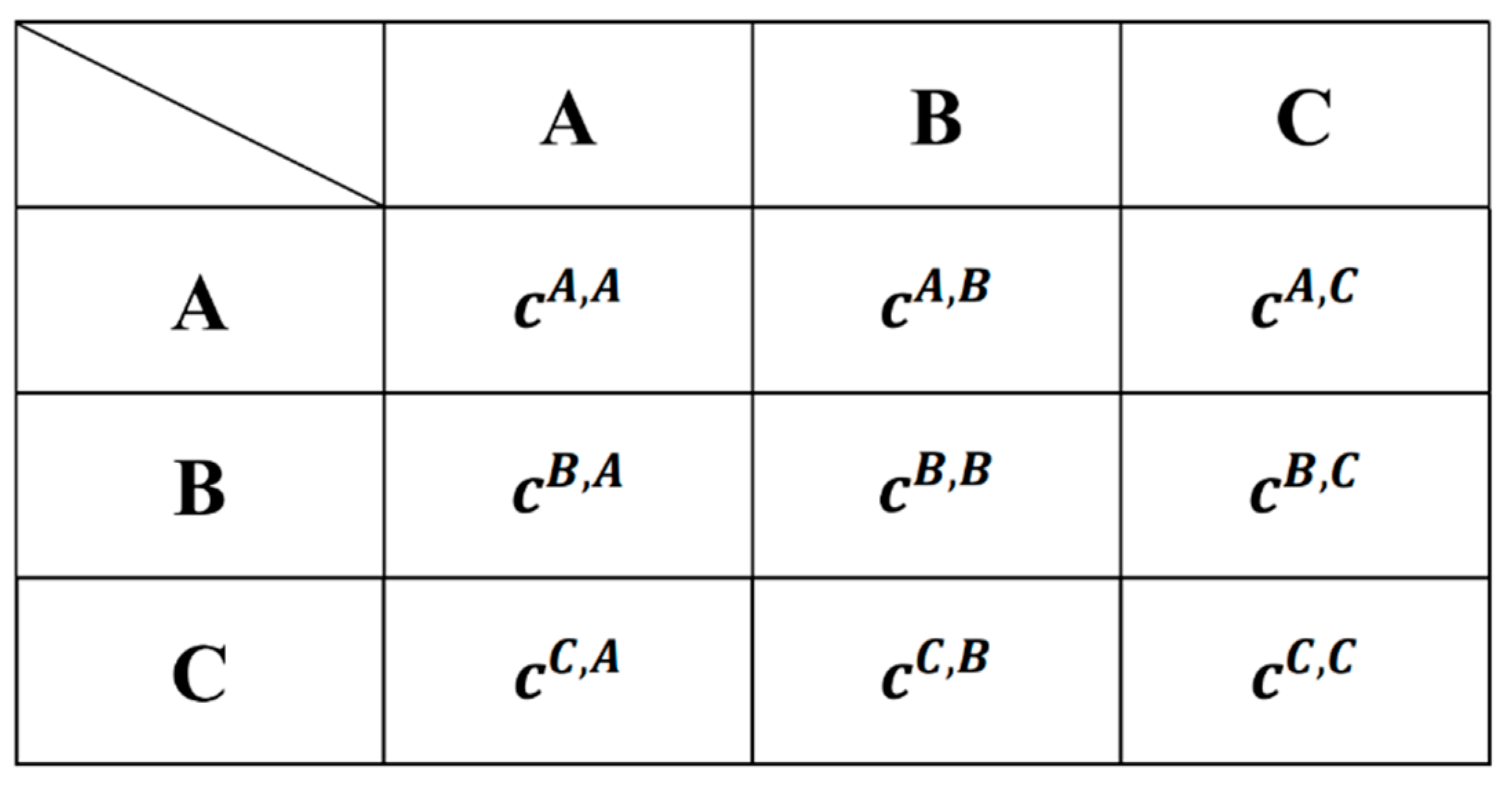
Figure 1 illustrated a simplified input–output table for carbon emissions:
In this table, taking region A as an example, the entries , , and represent the ACE generated by all products produced in region A. is the ACE generated by all products produced by region A for its own consumption, and are the ACE generated by all products produced by region A and consumed by regions B and C, indicating the embodied ACE exported by region A. Similarly, the entries , , and represent the ACE from the production of all products consumed in region A, indicating the ACE of region A based on the consumption side. and represent the ACE from the production of all products consumed by region A in regions B and C, representing the embodied ACE from imports in region A.
3.2. Logarithmic Mean Divisia Index Decomposition Method
The LMDI decomposition method is utilized to analyze the factors influencing the embodied ACE resulting from international trade between China and the United States. The LMDI is a more complete decomposition method than the SDA decomposition method, as it has no residuals and effectively avoids the pseudo-regression problem. The method is operational and adaptable, allows for effective analysis of overall indicators, has a flexible decomposition structure, and has the advantage of allowing for the presence of zero values in the data [40,41]. The selected influencing factors include intensity of embodied ACE per unit of traded products, the proportion of agricultural products in imports and exports, the proportion of the primary industry, GDP per capita, and the population size. The decomposition equation is as follows:
where:
- -
- and denote the embodied ACE from imported (exported) products and services.
- -
- and denote the amount of imported (exported) agricultural products.
- -
- denotes the gross agricultural product.
- -
- denotes the gross domestic product.
- -
- denotes the population size.
- -
- and represent the embodied ACE per unit dollar of imported (exported) products.
- -
- and represent the proportion of agricultural products in imports and exports.
- -
- γ denotes the proportion of the primary industry.
- -
- denotes the GDP per capita.
The changes in carbon emissions between the base period and the reporting period can be decomposed as follows:
According to the LMDI decomposition method, there is:
, , , , denote the variations in imports and exports of embodied ACE in international trade due to the changes in the intensity of imported (and exported) embodied ACE, the proportion of imported (and exported) agricultural products, the proportion of the primary industry, the GDP per capita, and the population size, respectively.
3.3. Data Sources
- Global Input–Output Tables. Because the EORA database covers more years (the EORA database covers global input–output data from 1990 to 2016) and more objects than WIOD, GTAP and other models, this study used the input–output tables of the EORA database [52,53] https://worldmrio.com/eora/ (accessed on 12 April 2023). Considering that the overall situation of global trade was basically stable before 1990, and taking into account the availability of data, the input–output tables for 1970 and 1980 are calculated using 1990 data.
- ACE Data. The data on ACE used in the study are from FAO [54]. In this paper, we refer to the IPCC national greenhouse gas emission inventory, and the calculated carbon emissions from agricultural production specifically include: Enteric Fermentation, Manure Management, Rice Cultivation, Synthetic Fertilizers, Manure applied to Soils, Manure left on Pasture, Crop Residues, Burning—Crop residues, Drained organic soils, Savanna fires.
- Global Agricultural Trade Volume. The global agricultural trade volume data is obtained from FAO [54].
- Gross primary sector product, gross domestic product, and population size for China and the United States are obtained from the World Bank database [55] https://databank.worldbank.org/reports.aspx?source=world-development-indicators (accessed on 12 April 2023). To eliminate the effects of price changes over time, agricultural trade volume, primary sector GDP, and GDP are all based on 1970 constant US dollars.
4. Results
4.1. ACE Based on Production and Consumption
The study calculated the ACE and the ACE per capita of China and the United States based on both the production and consumption sides using data from FAO and the input–output model. Table 1 and Table 2 present the results.
From 1970 to 2016, China’s ACE based on the production side and the consumption side both showed an upward trend, in which the ACE based on the production side increased from 400,904.57 kt to 700,933.54 kt, and those based on the consumption side increased from 382,109.91 kt to 741,280.79 kt. In 2000 and before, China’s ACE based on the production side were greater than those based on the consumption side; after 2000, ACE based on the production side were smaller than those based on the consumption side. Unlike China, consumption-based ACE has been higher than production-based ACE in the United States since 1980. The production-based ACE were 366,011.80 kt and consumption-based ACE were 362,389.51 kt in 1970, and climbed to 384,945.37 and 436,168.37 kt, respectively.
While China’s total ACE are consistently higher than the United States, ACE per capita in China are lower than those in the United States. In 1970, the United States’ ACE per capita based on production were about 3.70 times higher than China’s, and based on consumption, they were about 3.84 times higher. By 2016, the United States’ ACE per capita based on production were about 2.37 times higher than China’s, and based on consumption, they were about 2.54 times higher.
The trends in both countries showed that China’s ACE per capita based on production and consumption follow a rising and then declining pattern, with the peak values occurring in 2000 and 2010, respectively. On the other hand, the United States’ ACE per capita based on both production and consumption consistently decreased over time.
Comparing the ACE generated per unit of agricultural output value (constant 1970 USD price) in China and the United States, it is evident that both countries have significantly reduced emissions intensity over time. China’s emissions per unit of agricultural output value declined from 12.44 g/$ to 0.12 g/$, and the United States’ emissions declined from 18.41 g/$ to 0.45 g/$. Currently, China’s emissions intensity is only 26.67% of that in the United States, suggesting China’s efforts in promoting green agricultural production technologies and contributing to global agricultural carbon emission reductions (Figure 2).
4.2. Embodied ACE in China and the United States
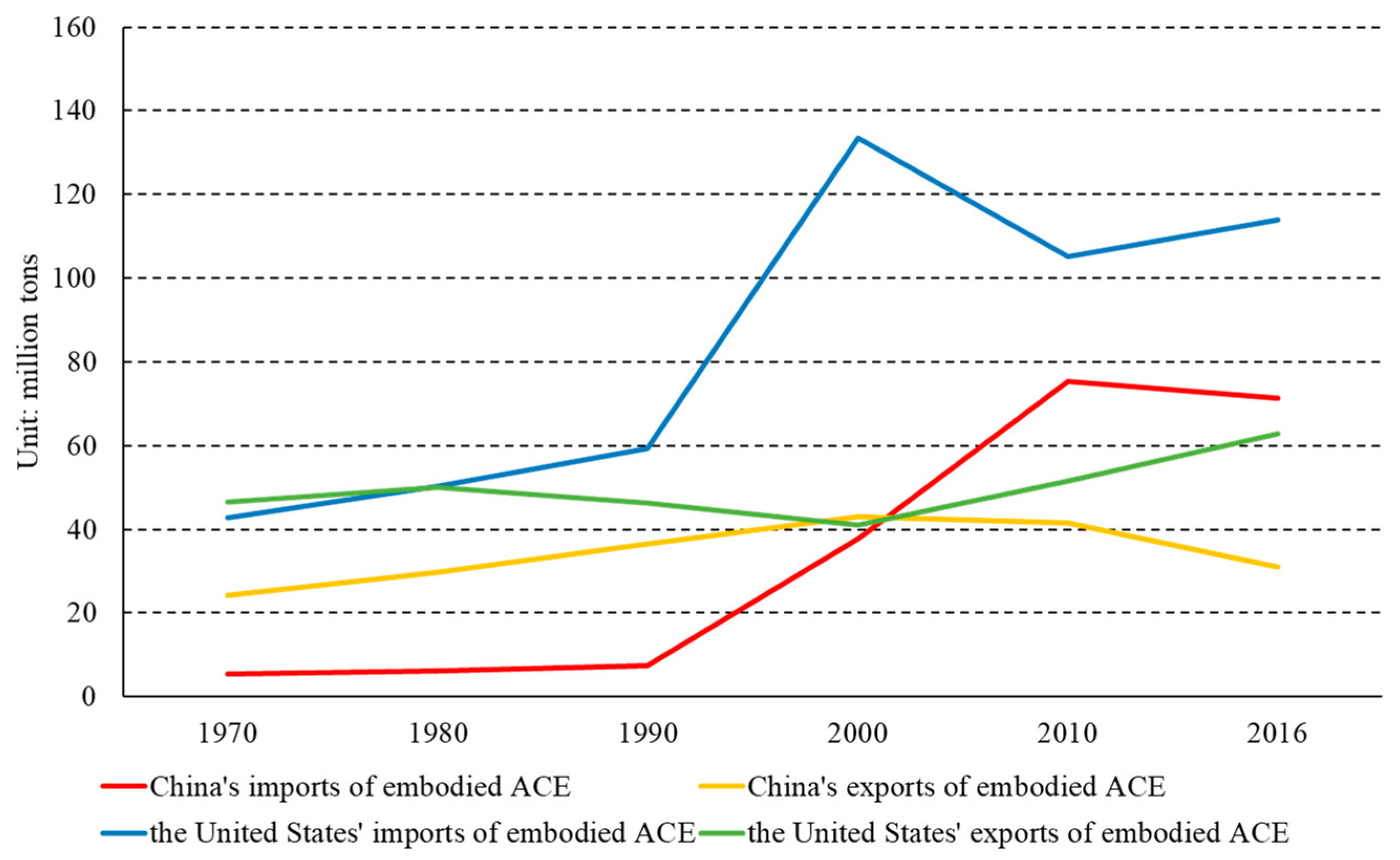
Regarding total imports and exports of embodied ACE, China’s international trade displayed an increasing and then decreasing trend from 1970 to 2016. Imports rose from 5535.74 kt in 1970 to 71,326.73 kt in 2016, peaking at 75,450.18 kt in 2010. Exports increased from 24,330.40 kt in 1970 to 30,979.47 kt in 2016, peaking at 43,131.66 kt in 2000. Figure 3 indicated that China’s net import of embodied ACE changed from negative to positive between 2000 and 2010, transforming from a net exporter to a net importer.
In contrast, the United States experienced fluctuations in embodied ACE imports and exports from 1970 to 2016. Imports increased from 42,884.00 kt in 1970 to 113,978.07 kt in 2016, with inflection points at 133,579.30 kt in 2000 and 10,504,949.70 kt in 2010. Exports increased from 46,506.29 kt in 1970 to 62,755.07 kt, with inflection points at 50,141.45 kt in 1980 and 41,025.15 kt in 2000. The United States transitioned from being a net exporter of embodied ACE to a net importer after 1980. The net imports of embodied ACE in the United States followed an upward trend until 2000 and then declined to 51,223.00 kt in 2016.
Overall, China’s total imports and exports of embodied ACE are lower than those of the United States. China became a net importer of embodied ACE during the 2000s, whereas the United States remained a net importer throughout the period.
4.3. Main Import and Export Targets for Embodied ACE in China and the United States
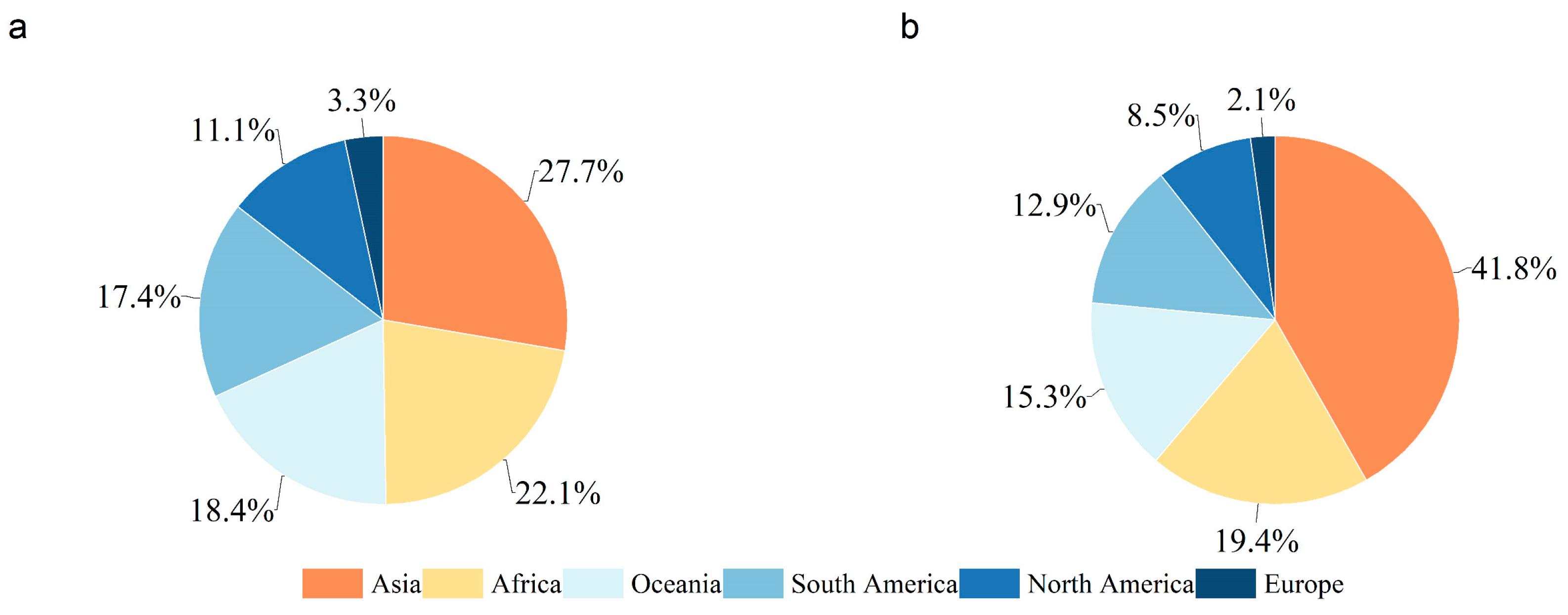
In this study, we identified the main import and export regions for embodied ACE in China and the United States. From 1970 to 2016, Asia consistently remained the largest recipient of China’s net imports of embodied ACE. However, the proportion of China’s net imports from Asia declined significantly from 82.07% in 1970 to 36.18% in 2016. In contrast, the proportions of net imports from Africa, Oceania, South America, North America, and Europe increased over the same period. These changes indicate that China’s trade connections have expanded beyond Asia and diversified globally (Figure 4 and Figure 5).
For the United States, the pattern of net imports of embodied ACE underwent considerable changes from 1970 to 2016. In 1970, the United States primarily imported embodied ACE from Asia, Africa, and South America. However, by 2016, the primary net importing regions shifted to Africa, North America, and Asia, while South America and Europe saw a slight decrease in their shares (Figure 6 and Figure 7).
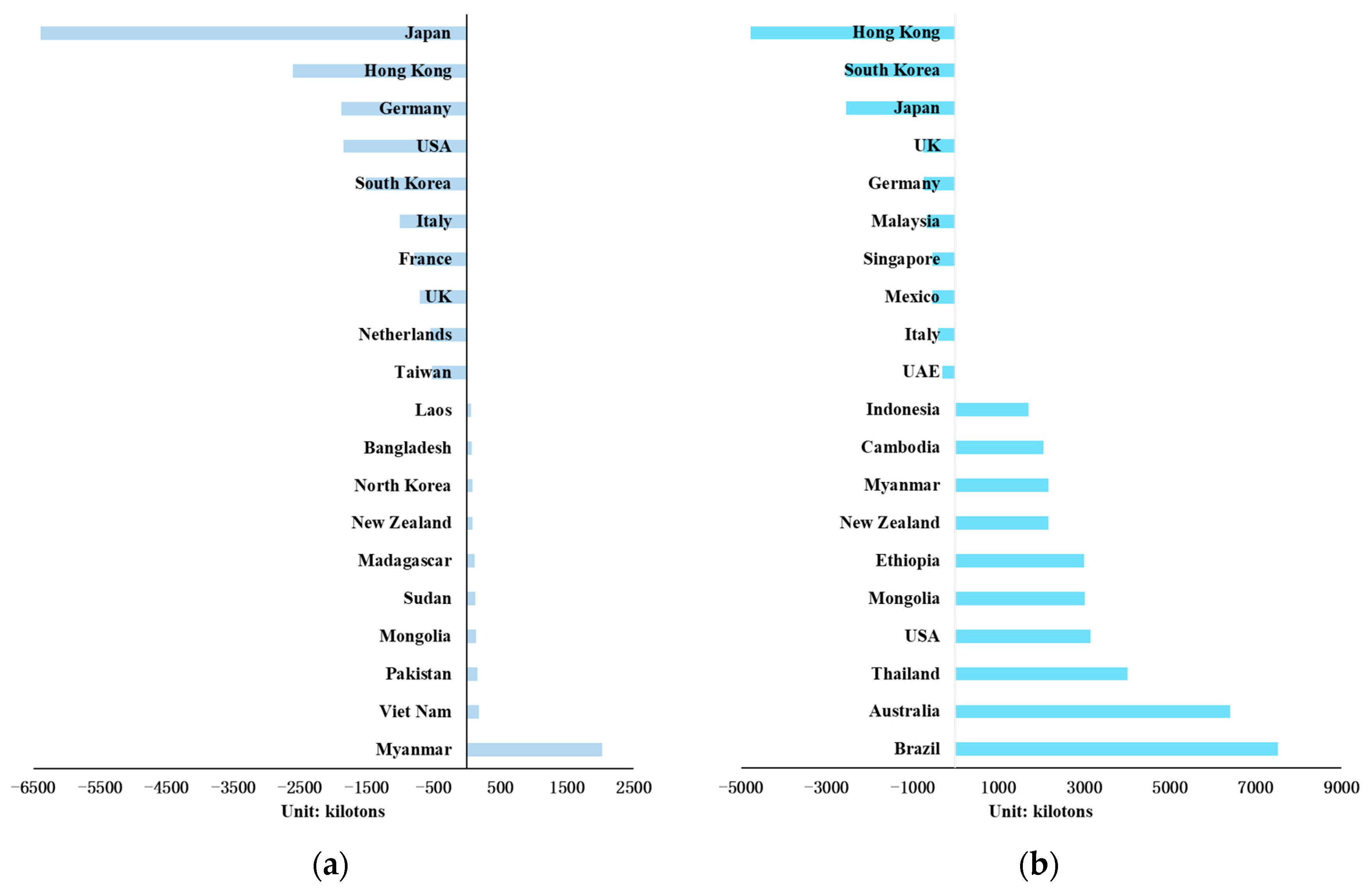
In terms of the main import and export targets of embodied ACE, in 1970, China’s major importers were Myanmar, Vietnam, and Pakistan, while its main export regions were Japan, Hong Kong (China), and Germany. In 2016, China’s major importers were Brazil, Australia, and Thailand, while its main export regions were Hong Kong (China), South Korea, and Japan. Interestingly, the United States was the major net importer of China’s embodied ACE in 1970, but it became the major net exporter to China in 2016 (Figure 8).
For the United States, its major net importing regions in 1970 were Canada, Madagascar, Argentina, and China, while the major net exporting regions were Japan, Taiwan, South Korea, and Mexico. By 2016, the major net importing regions shifted to Chad, Canada, Ethiopia, and Australia, while the major net exporting regions were Mexico, Japan, South Korea, and China (Figure 9).
4.4. Analysis of the Drivers of Embodied ACE from Imports and Exports in China and the United States
This study further analyzed the drivers of embodied ACE from imports and exports in both China and the United States using Equations (10)–(14).
For imports, in China, the factors influencing embodied ACE were mainly the suppression of embodied carbon intensity, the adjustment of the industrial structure, and the increase in GDP per capita. Similarly, in the United States, the main drivers were the suppression of embodied carbon intensity, the adjustment of the industrial structure, and the increase in GDP per capita.
For exports, in both China and the United States, the major drivers were an increase in GDP per capita, growth in population size, and changes in the proportion of export trade. The reduction in the intensity of embodied ACE and the adjustment of the industrial structure also contributed to reducing export ACE in both countries.
In this study, we found that both China and the United States shared common drivers for embodied ACE from imports and exports, which included changes in carbon intensity and industrial structure. Additionally, GDP per capita was a significant driver, leading to increased ACE for both countries. Population growth and changes in the proportion of agricultural products imported and exported also played roles in influencing embodied ACE, albeit to a lesser extent (Table 3 and Table 4).
5. Discussion
The discussion highlights some key findings and implications of our study’s results. Here are the main points:
(a) Disparities between China and the U.S.: This study reveals that China’s ACE, both based on production and consumption, are consistently higher than those of the United States. However, when considering per capita ACE, China’s values are lower than the U.S. This indicates that the U.S. has a higher carbon emission intensity per capita in the agricultural sector compared to China. China’s net imports of embodied ACE have also been consistently lower than those of the U.S. In 1970, China’s net exports of embodied ACE were 18.79 Mt, compared to 3.62 Mt for the U.S. In 2016, China’s net imports of embodied ACE were 40.35 Mt, compared to 51.22 Mt for the U.S. The U.S. is the largest importer of embodied ACE.
(b) Transition to Net Importers: Both China and the U.S. have transitioned from being net exporters to net importers of embodied ACE over time. This means that both countries are now importing more embodied ACE through their international trade activities.
(c) The Dominant Trading Partner: Both China and the U.S. primarily import and export embodied ACE with countries in the Asian region. While the share of imports and exports with other regions has changed over time, Asia remains a dominant trading partner.
(d) Driving Factors: This study identified several driving factors influencing embodied ACE, the decrease in embodied ACE intensity and the decrease in the proportion of primary industries as the main factors that reduce embodied ACE. Meanwhile, the increase in GDP per capita, the expansion of the population, and the increase in the proportion of agricultural products imported and exported all contribute to the increase in the embodied ACE of embodied agricultural carbon imports and exports. These results are consistent with the findings of previous studies [56,57,58,59].
6. Conclusions
Based on the analysis of the drivers of embodied ACE in China and the U.S., the following recommendations are proposed:
On the one hand, reduction of embodied ACE can be achieved by decreasing the intensity of such emissions and optimizing industrial structure.
(a) Continuously promote the research, development, and application of energy-saving and emission-reduction technologies. Agricultural technical progress was the major driving factor associated with decreases in ACE [60]. Improve relevant laws and regulations, and promote the introduction of foreign advanced energy-saving and emission-reduction technologies [61,62,63]; we should strongly support enterprises, scientific research institutes, and colleges and universities to carry out research and development and production of energy-saving and emission-reduction technologies, to achieve genuine collaboration between industry, academia, and research. We should increase the support of educational policies on energy-saving and emission reduction, open specialties and disciplines related to energy-saving and emission reduction, and cultivate highly skilled talents in energy-saving and emission reduction.
(b) Optimize industrial structure. Industrial structure is a critical factor affecting the low-carbon development of cities [58]. China should further focus on industrial policy guidance and optimization of energy structure, allocate special financial funds to strengthen the protection of clean industry projects, accelerate the construction of big data, artificial intelligence, and other digital technologies, promote the digital economy and digital technology to the traditional high-energy-consuming industries, and improve the efficiency of carbon emissions.
On the other hand, implementation of relevant energy-saving and emission-reduction policies should be promoted. Governments can establish programs and funds to reduce the financial pressure on enterprises’ scientific and technological innovation, encourage countries worldwide to actively develop new energy products, and promote the conversion of scientific and technological achievements into practical applications. Embodied ACE can also be reduced by encouraging behaviors such as minimizing food waste [47,64,65].
Finally, the shortcomings of this paper are presented: First, this paper is a study that used only six years of input–output tables in 1970, 1980, 1990, 2000, 2010, and 2016, without continuous measurement for all years, and the conclusions obtained are still relatively shallow. Second, this paper has analyzed the degree of influence of the influencing factors using the LMDI decomposition method, but the discussion of the influencing factors could be more specific. Econometric analysis methods and SDA methods should be added to future research on the impact factors of implied carbon emissions, and different results should be compared and discussed to enrich the research in this area.
Author Contributions
R.S. analyzed the data and drafted the manuscript; J.L., K.N. and Y.F. completed the manuscript and made major revisions. All authors have read and agreed to the published version of the manuscript.
Funding
This research was funded by National Key Research and Development Program, Intergovernmental Cooperation in International Science and Technology Innovation/Key Project of Hong Kong, Macao and Taiwan Science and Technology Innovation Cooperation, “Sino-Thai Cooperation on Community Water Management for Climate Change Adaptation”: 2017YFE0133000; Chinese Academy of Agricultural Sciences Science and Technology Innovation Project (10-IAED-06-2023); Fundamental Research Funds for Central Public Welfare Research Institutes (Y2022ZK03).
Institutional Review Board Statement
Not applicable.
Data Availability Statement
The data that support the findings of this study are available in the article itself.
Conflicts of Interest
The authors declare no conflict of interest.
References
- Davidson, E.A. The contribution of manure and fertilizer nitrogen to atmospheric nitrous oxide since 1860. Nat. Geosci. 2009, 2, 659–662. [Google Scholar] [CrossRef]
- Foley, J.A.; Ramankutty, N.; Brauman, K.A.; Cassidy, E.S.; Gerber, J.S.; Johnston, M.; Mueller, N.D.; O Connell, C.; Ray, D.K.; West, P.C.; et al. Solutions for a cultivated planet. Nature 2011, 478, 337–342. [Google Scholar] [CrossRef] [PubMed]
- Liu, Y.; Tang, H.; Muhammad, A.; Huang, G. Emission mechanism and reduction countermeasures of agricultural greenhouse gases—A review. Greenh. Gases-Sci. Technol. 2019, 9, 160–174. [Google Scholar] [CrossRef]
- Hatab, A.A.; Bustamante, M.; Clark, H.; Havlík, P.; House, J.; Mbow, C.; Ninan, K.N.; Popp, A.; Roe, S.; Sohngen, B.; et al. WG III Contribution to the Sixth Assessment Report: Chapter 7: Agriculture, Forestry and Other Land Uses (AFOLU)[R]. Available online: https://www.ipcc.ch/report/ar6/wg3/downloads/report/IPCC_AR6_WGIII_Chapter_07.pdf (accessed on 1 March 2023).
- Le Quéré, C.; Raupach, M.R.; Canadell, J.G.; Marland, G.; Bopp, L.; Ciais, P.; Conway, T.J.; Doney, S.C.; Feely, R.A.; Foster, P.; et al. Trends in the sources and sinks of carbon dioxide. Nat. Geosci. 2009, 2, 831–836. [Google Scholar] [CrossRef]
- Hertwich, E.G.; Peters, G.P. Carbon Footprint of Nations: A Global, Trade-Linked Analysis. Environ. Sci. Technol. 2009, 43, 6414–6420. [Google Scholar] [CrossRef]
- Davis, S.J.; Caldeira, K. Consumption-based accounting of CO2 emissions. Proc. Natl. Acad. Sci. USA 2010, 107, 5687–5692. [Google Scholar] [CrossRef]
- Peters, G.P.; Minx, J.C.; Weber, C.L.; Edenhofer, O. Growth in emission transfers via international trade from 1990 to 2008. Proc. Natl. Acad. Sci. USA 2011, 108, 8903–8908. [Google Scholar] [CrossRef]
- Zhao, X.; Wu, X.; Guan, C.; Ma, R.; Nielsen, C.P.; Zhang, B. Linking Agricultural GHG Emissions to Global Trade Network. Earth’s Future 2020, 8, e2019EF001361. [Google Scholar] [CrossRef]
- Han, M.; Zhang, B.; Zhang, Y.; Guan, C. Agricultural CH4 and N2O emissions of major economies: Consumption-vs. production-based perspectives. J. Clean. Prod. 2019, 210, 276–286. [Google Scholar] [CrossRef]
- Song, R.; Liu, J.; Niu, K. Agricultural Carbon Emissions Embodied in China’s Foreign Trade and Its Driving Factors. Sustainability 2023, 15, 787. [Google Scholar] [CrossRef]
- Liu, Y.; Yan, C.; Gao, J.; Wu, X.; Zhang, B. Mapping the changes of CH4 emissions in global supply chains. Sci. Total Environ. 2022, 832, 155019. [Google Scholar] [CrossRef] [PubMed]
- Sun, X.; Cheng, X.; Guan, C.; Wu, X.; Zhang, B. Economic drivers of global and regional CH4 emission growth from the consumption perspective. Energy Policy 2022, 170, 113242. [Google Scholar] [CrossRef]
- Grimm, N.B.; Faeth, S.H.; Golubiewski, N.E.; Redman, C.L.; Wu, J.; Bai, X.; Briggs, J.M. Global Change and the Ecology of Cities. Science 2008, 319, 756–760. [Google Scholar] [CrossRef] [PubMed]
- Gurney, K.R.; Romero-Lankao, P.; Seto, K.C.; Hutyra, L.R.; Duren, R.; Kennedy, C.; Grimm, N.B.; Ehleringer, J.R.; Marcotullio, P.; Hughes, S.; et al. Climate change: Track urban emissions on a human scale. Nature 2015, 525, 179–181. [Google Scholar] [CrossRef] [PubMed]
- Chen, S.; Chen, B.; Feng, K.; Liu, Z.; Fromer, N.; Tan, X.; Alsaedi, A.; Hayat, T.; Weisz, H.; Schellnhuber, H.J.; et al. Physical and virtual carbon metabolism of global cities. Nat. Commun. 2020, 11, 182. [Google Scholar] [CrossRef] [PubMed]
- Li, Y.; Zhong, H.; Shan, Y.; Hang, Y.; Wang, D.; Zhou, Y.; Hubacek, K. Changes in global food consumption increase GHG emissions despite efficiency gains along global supply chains. Nat. Food 2023, 4, 483–495. [Google Scholar] [CrossRef]
- Balié, J.; Del Prete, D.; Magrini, E.; Montalbano, P.; Nenci, S. Does Trade Policy Impact Food and Agriculture Global Value Chain Participation of Sub-Saharan African Countries? Am. J. Agric. Econ. 2019, 101, 773–789. [Google Scholar] [CrossRef]
- Geng, Y.; Dong, H.J.; Xi, F.M.; Liu, Z. A Review of the Research on Carbon Footprint Responding to Climate Change. China Popul. Resour. Environ. 2010, 20, 6–12. [Google Scholar]
- Tu, J.; Zhu, Z. Research on the Impact of Grain Trade on China’s Embodied Carbon Emissions. World Agric. 2023, 82–92. [Google Scholar] [CrossRef]
- Leontief, W. Environmental Repercussions and the Economic Structure: An Input-Output Approach; Routledge: London, UK, 1970; Volume 52, pp. 262–271. [Google Scholar]
- Yan, Y.; Wang, R.; Zheng, X.; Zhao, Z. Carbon endowment and trade-embodied carbon emissions in global value chains: Evidence from China. Appl. Energy 2020, 277, 115592. [Google Scholar] [CrossRef]
- Hong, C.; Zhao, H.; Qin, Y.; Burney, J.A.; Pongratz, J.; Hartung, K.; Liu, Y.; Moore, F.C.; Jackson, R.B.; Zhang, Q.; et al. Land-use emissions embodied in international trade. Science 2022, 376, 597–603. [Google Scholar] [CrossRef] [PubMed]
- Li, R.; Zhang, J.; Krebs, P. Global trade drives transboundary transfer of the health impacts of polycyclic aromatic hydrocarbon emissions. Commun. Earth Environ. 2022, 3, 170. [Google Scholar] [CrossRef] [PubMed]
- Liu, H.; Liu, W.; Fan, X.; Zou, W. Carbon emissions embodied in demand–supply chains in China. Energy Econ. 2015, 50, 294–305. [Google Scholar] [CrossRef]
- Liu, Y.; Meng, B.; Hubacek, K.; Xue, J.; Feng, K.; Gao, Y. ‘Made in China’: A reevaluation of embodied CO2 emissions in Chinese exports using firm heterogeneity information. Appl. Energy 2016, 184, 1106–1113. [Google Scholar] [CrossRef]
- Lin, J.; Du, M.; Chen, L.; Feng, K.; Liu, Y.; Martin, R.V.; Wang, J.; Ni, R.; Zhao, Y.; Kong, H.; et al. Carbon and health implications of trade restrictions. Nat. Commun. 2019, 10, 4947. [Google Scholar] [CrossRef]
- Peng, S.; Zhang, W.; Sun, C. China’s Production-Based and Consumption-Based Carbon Emissions and Their Determinants. Econ. Res. J. 2015, 50, 168–182. [Google Scholar]
- Peters, G.P.; Hertwich, E.G. CO2 Embodied in International Trade with Implications for Global Climate Policy. Environ. Sci. Technol. 2008, 42, 1401–1407. [Google Scholar] [CrossRef]
- Li, Y.; Hewitt, C.N. The effect of trade between China and the UK on national and global carbon dioxide emissions. Energy Policy 2008, 36, 1907–1914. [Google Scholar] [CrossRef]
- Meng, J.; Mi, Z.; Guan, D.; Li, J.; Tao, S.; Li, Y.; Feng, K.; Liu, J.; Liu, Z.; Wang, X.; et al. The rise of South–South trade and its effect on global CO2 emissions. Nat. Commun. 2018, 9, 1871. [Google Scholar] [CrossRef]
- Zhao, Y.; Wang, S.; Zhang, Z.; Liu, Y.; Ahmad, A. Driving factors of carbon emissions embodied in China–US trade: A structural decomposition analysis. J. Clean. Prod. 2016, 131, 678–689. [Google Scholar] [CrossRef]
- Bin, S.; Dowlatabadi, H. Consumer lifestyle approach to US energy use and the related CO2 emissions. Energy Policy 2005, 33, 197–208. [Google Scholar] [CrossRef]
- Feng, K.; Davis, S.J.; Sun, L.; Li, X.; Guan, D.; Liu, W.; Liu, Z.; Hubacek, K. Outsourcing CO2 within China. Proc. Natl. Acad. Sci. USA 2013, 110, 11654–11659. [Google Scholar] [CrossRef]
- Mongelli, I.; Tassielli, G.; Notarnicola, B. Global warming agreements, international trade and energy/carbon embodiments: An input–output approach to the Italian case. Energy Policy 2006, 34, 88–100. [Google Scholar] [CrossRef]
- Peters, G.P.; Hertwich, E.G. Pollution embodied in trade: The Norwegian case. Glob. Environ. Chang. 2006, 16, 379–387. [Google Scholar] [CrossRef]
- Su, B.; Ang, B.W.; Li, Y. Input-output and structural decomposition analysis of Singapore’s carbon emissions. Energy Policy 2017, 105, 484–492. [Google Scholar] [CrossRef]
- Pan, W.; Pan, W.; Shi, Y.; Liu, S.; He, B.; Hu, C.; Tu, H.; Xiong, J.; Yu, D. China’s inter-regional carbon emissions: An input-output analysis under considering national economic strategy. J. Clean. Prod. 2018, 197, 794–803. [Google Scholar] [CrossRef]
- Su, B.; Ang, B.W. Structural decomposition analysis applied to energy and emissions: Some methodological developments. Energy Econ. 2012, 34, 177–188. [Google Scholar] [CrossRef]
- Deng, G.; Lu, F.; Yue, X. Research on China’s embodied carbon import and export trade from the perspective of value-added trade. PLoS ONE 2021, 16, e258902. [Google Scholar] [CrossRef]
- Yang, W.; Gao, H.; Yang, Y. Analysis of Influencing Factors of Embodied Carbon in China’s Export Trade in the Background of “Carbon Peak” and “Carbon Neutrality”. Sustainability 2022, 14, 3308. [Google Scholar] [CrossRef]
- Hillman, T.; Ramaswami, A. Greenhouse Gas Emission Footprints and Energy Use Benchmarks for Eight U.S. Cities. Environ. Sci. Technol. 2010, 44, 1902–1910. [Google Scholar] [CrossRef] [PubMed]
- Ren, S.; Yuan, B.; Ma, X.; Chen, X. International trade, FDI (foreign direct investment) and embodied CO2 emissions: A case study of Chinas industrial sectors. China Econ. Rev. 2014, 28, 123–134. [Google Scholar] [CrossRef]
- Mi, Z.; Meng, J.; Guan, D.; Shan, Y.; Song, M.; Wei, Y.; Liu, Z.; Hubacek, K. Chinese CO2 emission flows have reversed since the global financial crisis. Nat. Commun. 2017, 8, 1712. [Google Scholar] [CrossRef] [PubMed]
- Chontanawat, J.; Wiboonchutikula, P.; Buddhivanich, A. An LMDI decomposition analysis of carbon emissions in the Thai manufacturing sector. Energy Rep. 2020, 6, 705–710. [Google Scholar] [CrossRef]
- Wang, S.; Li, Z.; Song, M. How embodied carbon in trade affects labor income in developing countries. Sci. Total Environ. 2019, 672, 71–80. [Google Scholar] [CrossRef]
- Hotak, S.; Islam, M.; Kakinaka, M.; Kotani, K. Carbon emissions and carbon trade balances: International evidence from panel ARDL analysis. Environ. Sci. Pollut. Res. 2020, 27, 24115–24128. [Google Scholar] [CrossRef]
- Li, C.; Li, H.Y.; Kong, H.Z.; Feng, W. Structural characteristics and driving factors of embodied carbon emissions from fishery production system in China. Resour. Sci. 2021, 43, 1166–1177. [Google Scholar] [CrossRef]
- Malik, A.; McBain, D.; Wiedmann, T.O.; Lenzen, M.; Murray, J. Advancements in Input-Output Models and Indicators for Consumption-Based Accounting. J. Ind. Ecol. 2019, 23, 300–312. [Google Scholar] [CrossRef]
- Weinzettel, J.; Steen-Olsen, K.; Hertwich, E.G.; Borucke, M.; Galli, A. Ecological footprint of nations: Comparison of process analysis, and standard and hybrid multiregional input–output analysis. Ecol. Econ. 2014, 101, 115–126. [Google Scholar] [CrossRef]
- Usubiaga-Liaño, A.; Arto, I.; Acosta-Fernández, J. Double accounting in energy footprint and related assessments: How common is it and what are the consequences? Energy 2021, 222, 119891. [Google Scholar] [CrossRef]
- Lenzen, M.; Moran, D.; Kanemoto, K.; Geschke, A. Building eora: A global multi-region input-output database at high country and sector resolution. Econ. Syst. Res. 2013, 25, 20–49. [Google Scholar] [CrossRef]
- Lenzen, M.; Kanemoto, K.; Moran, D.; Geschke, A. Mapping the Structure of the World Economy. Environ. Sci. Technol. 2012, 46, 8374–8381. [Google Scholar] [CrossRef] [PubMed]
- FAO. FAOSTAT Climate Change, Emissions, Emissions Totals. 2022. Available online: https://www.fao.org/faostat/en/#data/GT (accessed on 12 April 2023).
- World Bank. World Development Indicators 2017; License: Creative Commons Attribution CC BY 3.0 IGO; World Bank: Washington, DC, USA, 2017. [Google Scholar]
- Rüstemoğlu, H. Analysis of the drivers of CO2 emissions and ecological footprint growth in Australia. Energy Effic. 2022, 15, 1. [Google Scholar] [CrossRef] [PubMed]
- Rüstemoğlu, H. Factors affecting Germany’s green development over 1990–2015: A comprehensive environmental analysis. Environ. Sci. Pollut. Res. 2019, 26, 6636–6651. [Google Scholar] [CrossRef]
- Guo, H.; Fan, B.; Pan, C. Study on Mechanisms Underlying Changes in Agricultural Carbon Emissions: A Case in Jilin Province, China, 1998–2018. Int. J. Environ. Res. Public Health 2021, 18, 919. [Google Scholar] [CrossRef]
- He, J.; Yang, Y.; Liao, Z.; Xu, A.; Fang, K. Linking SDG 7 to assess the renewable energy footprint of nations by 2030. Appl. Energy 2022, 317, 119167. [Google Scholar] [CrossRef]
- Han, H.; Zhong, Z.; Guo, Y.; Xi, F.; Liu, S. Coupling and decoupling effects of agricultural carbon emissions in China and their driving factors. Environ. Sci. Pollut. Res. 2018, 25, 25280–25293. [Google Scholar] [CrossRef]
- Huang, W.; Wu, F.; Han, W.; Li, Q.; Han, Y.; Wang, G.; Feng, L.; Li, X.; Yang, B.; Lei, Y.; et al. Carbon footprint of cotton production in China: Composition, spatiotemporal changes and driving factors. Sci. Total Environ. 2022, 821, 153407. [Google Scholar] [CrossRef]
- Haller, A. Influence of Agricultural Chains on the Carbon Footprint in the Context of European Green Pact and Crises. Agriculture 2022, 12, 751. [Google Scholar] [CrossRef]
- Savino, M.M.; Manzini, R.; Mazza, A. Environmental and economic assessment of fresh fruit supply chain through value chain analysis. A case study in chestnuts industry. Prod. Plan. Control 2015, 26, 1–18. [Google Scholar] [CrossRef]
- Liu, C.; Shang, J.; Liu, C. Exploring Household Food Waste Reduction for Carbon Footprint Mitigation: A Case Study in Shanghai, China. Foods 2023, 12, 3211. [Google Scholar] [CrossRef]
- Brancoli, P.; Rousta, K.; Bolton, K. Life cycle assessment of supermarket food waste. Resour. Conserv. Recycl. 2017, 118, 39–46. [Google Scholar] [CrossRef]
Figure 1.
The structure of an MRIO model for carbon emissions.

Figure 2.
ACE per unit of agricultural output in China and the United States.

Figure 3.
Embodied ACE imports and exports of China and the United States.

Figure 4.
Regions of embodied ACE in China, 1970: (a) Net imports; (b) Net exports.

Figure 5.
Regions of embodied ACE in China, 2016: (a) Net imports; (b) Net exports.

Figure 6.
Regions of embodied ACE in the United States, 1970: (a) Net imports; (b) Net exports.

Figure 7.
Regions of embodied ACE in the United States, 2016: (a) Net imports; (b) Net exports.

Figure 8.
Main importers and exporters of embodied ACE in China: (a) 1970; (b) 2016.

Figure 9.
Main importers and exporters of embodied ACE in the United States: (a) 1970; (b) 2016.


Table 1.
ACE in China and the United States based on the production and consumption side *.
| Year | China | The United States | ||
|---|---|---|---|---|
| Production Side | Consumption Side | Production Side | Consumption Side | |
| 1970 | 400,904.57 | 382,109.91 | 366,011.80 | 362,389.51 |
| 1980 | 490,130.40 | 466,656.13 | 394,621.07 | 394,696.60 |
| 1990 | 602,906.60 | 573,853.52 | 363,642.05 | 376,812.42 |
| 2000 | 688,122.03 | 682,713.32 | 374,275.25 | 466,829.41 |
| 2010 | 698,246.30 | 732,199.10 | 378,351.88 | 431,883.61 |
| 2016 | 700,933.54 | 741,280.79 | 384,945.37 | 436,168.37 |
* Measured in kilotons.
Table 2.
ACE per capita in China and the United States based on the production and consumption side *.
Table 2.
ACE per capita in China and the United States based on the production and consumption side *.
| Year | China | The United States | ||
|---|---|---|---|---|
| Production Side | Consumption Side | Production Side | Consumption Side | |
| 1970 | 0.4831 | 0.4604 | 1.7850 | 1.7673 |
| 1980 | 0.4966 | 0.4728 | 1.7367 | 1.7370 |
| 1990 | 0.5273 | 0.5019 | 1.4568 | 1.5095 |
| 2000 | 0.5429 | 0.5387 | 1.3265 | 1.6545 |
| 2010 | 0.5207 | 0.5460 | 1.2231 | 1.3962 |
| 2016 | 0.5034 | 0.5324 | 1.1915 | 1.3501 |
* Measured in kilotons.
Table 3.
ACE per capita in China and the United States based on the production and consumption side *.
Table 3.
ACE per capita in China and the United States based on the production and consumption side *.
| Period | The Imports of China | The Imports of the United States | ||||||||
|---|---|---|---|---|---|---|---|---|---|---|
| Intensity of Embodied ACE | Proportion of Agricultural Products | Proportion of the Primary Industry | GDP per Capita | Population | Intensity of Embodied ACE | Proportion of Agricultural Products | Proportion of the Primary Industry | GDP per Capita | Population | |
| 1970–1980 | −13,556.5 | −104,443 | −104,443 | −104,443 | −104,443 | −104,443 | 21,211.91 | −4329.11 | 17,537.98 | 4672.427 |
| 1980–1990 | −1916.1 | −15,527 | −15,527 | −15,527 | −15,527 | −15,527 | 11,312.64 | −3589.19 | 33,541.5 | 4857.603 |
| 1990–2000 | 6141.584 | 34,931.44 | 34,931.44 | 34,931.44 | 34,931.44 | 34,931.44 | −10,109.4 | −23,627.7 | 71,043.99 | 4098.252 |
| 2000–2010 | −91,879.9 | −237,826 | −237,826 | −237,826 | −237,826 | −237,826 | −5329.33 | −19,187.6 | 83,274.36 | 2384.434 |
| 2010–2016 | −40,606.1 | −37,180.9 | −37,180.9 | −37,180.9 | −37,180.9 | −37,180.9 | −1894.44 | −5258.66 | 25,957.51 | 1353.77 |
| 1970–2016 | −141,817 | −360,046 | −360,046 | −360,046 | −360,046 | −360,046 | 15,191.35 | −55,992.3 | 231,355.3 | 17,366.49 |
* Measured in kilotons.
Table 4.
ACE per capita in China and the United States based on the production and consumption side *.
Table 4.
ACE per capita in China and the United States based on the production and consumption side *.
| Period | The Exports of China | The Exports of the United States | ||||||||
|---|---|---|---|---|---|---|---|---|---|---|
| Intensity of Embodied ACE | Proportion of Agricultural Products | Proportion of the Primary Industry | GDP per Capita | Population | Intensity of Embodied ACE | Proportion of Agricultural Products | Proportion of the Primary Industry | GDP per Capita | Population | |
| 1970–1980 | −33,678.2 | 21,211.91 | −4329.11 | 17,537.98 | 4672.427 | −112,832 | 41,992.17 | −5077.56 | 74,593.52 | 4959.414 |
| 1980–1990 | −39,278.3 | 11,312.64 | −3589.19 | 33,541.5 | 4857.603 | −26,450.1 | −24,011.6 | −8617.06 | 50,616.25 | 4526.304 |
| 1990–2000 | −34,863 | −10,109.4 | −23,627.7 | 71,043.99 | 4098.252 | −23,409.5 | −5889.25 | −8366.76 | 27,147.59 | 5337.924 |
| 2000–2010 | −62,776.2 | −5329.33 | −19,187.6 | 83,274.36 | 2384.434 | −33,520.4 | 21,817.66 | −5125.05 | 23,085.75 | 4234.836 |
| 2010–2016 | −30,676.1 | −1894.44 | −5258.66 | 25,957.51 | 1353.77 | −2190.57 | 683.0044 | −5016.33 | 15,285.01 | 2475.984 |
| 1970–2016 | −201,272 | 15,191.35 | −55,992.3 | 231,355.3 | 17,366.49 | −198,403 | 34,591.96 | −32,202.8 | 190,728.1 | 21,534.46 |
* Measured in kilotons.
Disclaimer/Publisher’s Note: The statements, opinions and data contained in all publications are solely those of the individual author(s) and contributor(s) and not of MDPI and/or the editor(s). MDPI and/or the editor(s) disclaim responsibility for any injury to people or property resulting from any ideas, methods, instructions or products referred to in the content. |
© 2023 by the authors. Licensee MDPI, Basel, Switzerland. This article is an open access article distributed under the terms and conditions of the Creative Commons Attribution (CC BY) license (https://creativecommons.org/licenses/by/4.0/).
Share and Cite
MDPI and ACS Style
Song, R.; Liu, J.; Niu, K.; Feng, Y. Comparative Analysis of Trade’s Impact on Agricultural Carbon Emissions in China and the United States. Agriculture 2023, 13, 1967. https://doi.org/10.3390/agriculture13101967
AMA Style
Song R, Liu J, Niu K, Feng Y. Comparative Analysis of Trade’s Impact on Agricultural Carbon Emissions in China and the United States. Agriculture. 2023; 13(10):1967. https://doi.org/10.3390/agriculture13101967
Chicago/Turabian StyleSong, Rui, Jing Liu, Kunyu Niu, and Yiyu Feng. 2023. "Comparative Analysis of Trade’s Impact on Agricultural Carbon Emissions in China and the United States" Agriculture 13, no. 10: 1967. https://doi.org/10.3390/agriculture13101967
Note that from the first issue of 2016, this journal uses article numbers instead of page numbers. See further details here.