
Design and Experiment of Adaptive Profiling Header Based on Multi-Body Dynamics–Discrete Element Method Coupling
1
Key Laboratory of Modern Agricultural Equipment and Technology, Ministry of Education, Jiangsu University, Zhenjiang 212013, China
2
College of Engineering, South China Agricultural University, Guangzhou 510642, China
*
Author to whom correspondence should be addressed.
Agriculture 2024, 14(1), 105; https://doi.org/10.3390/agriculture14010105
Submission received: 8 December 2023
/
Revised: 4 January 2024
/
Accepted: 5 January 2024
/
Published: 8 January 2024
(This article belongs to the Special Issue From Planting to Harvesting: The Role of Agricultural Machinery in Crop Cultivation)
Abstract
:To promote the germination of rice panicles during the regeneration season, it is necessary to ensure a stubble height of 300–450 mm when mechanically harvesting the first-season rice. However, due to variations in the depth of the paddy soil and fluctuations in the height of the header during harvesting, maintaining the desired stubble height becomes challenging, resulting in a significant impact on the yield during the regeneration season. This study presents the design of an adaptive profiling header capable of adjusting the height and level of the header adaptively. Based on the theoretical analysis of the profiling mechanism, a quadratic regression orthogonal rotation combination experiment is designed. Considering the actual field conditions, the range of each factor is determined, and simulation experiments are conducted based on the MBD-DEM coupling to establish a mathematical regression model between each factor and indicator. In the case of the profiling wheel linkage length of 562 mm, profiling wheel width of 20 mm, and profiling wheel mass of 3.6 kg, the supporting force of the header on the profiling wheel would be greater than zero, the supporting force of soil on the profiling wheel and the depth of soil subsidence represent the smallest values, and the highest sensitivity and accuracy of the profiling wheel are achieved. Bench tests demonstrated that the header exerts a force on the profiling wheel, confirming the normal functioning of the profiling. The average magnitudes of forces exerted by the soil on the profiling wheel are obtained to be 31.98 N, 31.63 N, and 30.86 N, whereas the corresponding average soil subsidence depths are obtained as 3.4 mm, 5.6 mm, and 8.3 mm, aligning closely with the simulation values. The results indicate that the profiling mechanism achieves high accuracy in ground profiling and that the structural design is reasonable. By employing fuzzy PID control to adjust the height of the header, the average error in adjustment is obtained as 6.75 mm, while the average error in the horizontal adjustment is derived as 0.64°. The header adjustment is fast, offering high positioning accuracy, thereby meeting the harvesting requirements of the first season of ratooning rice.
1. Introduction
Ratooning rice has several advantages, including dual harvest, labor and planting saving, optimal use of light and temperature resources, increased grain yield and income, and improved rice quality [1,2,3]. It has gained rapid popularity in the middle and lower reaches of the Yangtze River [4,5,6,7].
During the mechanized harvesting of the first season of ratooning rice, it is crucial to maintain a specific stubble height [8,9], typically ranging from 300 to 450 mm, depending on the rice variety [10,11,12]. During the harvesting of ratooning rice, the soil depth and the height of the harvester’s header can vary across different fields. To ensure consistent stubble height, the harvester driver needs to make real-time adjustments to the header height. Uneven stubble height can negatively impact the efficiency of the operation and the tiller growth during the ratooning season. Thus, an adaptive profiling header is needed on the ratooning rice harvester, which can automatically adjust the height and level of the header based on undulating ground conditions. This adjustment ensures consistent stubble height, leading to improved yield during the ratooning season.
Investigators at home and abroad have researched the automatic adjustment of the cutting height of a combine harvester’s cutting profile system. Tulpule et al. designed a combine harvester header height control system based on the integrated robust optimal design (IROD) method [13], whereas Kassen et al. employed the robust feedback linearization (RFL) approach to enhance the robustness of the header height control system while reducing the control system power consumption [14]. Ni et al. designed an adaptive control system for the height of the soybean combine harvester based on a soil machine system, with an accuracy of 92% for the header contour control [15]. The above research works are mainly focused on the control strategy and control algorithm research of the header profiling system, rather than structural design. Additionally, due to the complexity of the planting environment for ratooning rice, the above research has poor adaptability to the harvesting of ratooning rice.
To achieve higher yield in the rice regeneration season and enable the adaptive profiling control of the header, this paper establishes a design approach for an adaptive profiling header. Because the movement of soil particles is very complicated and irregular, the software EDEM (2020, DEM-Solutions Ltd., Edinburgh, UK) and RecurDyn (V9R2, Function Bay Ltd., Seongnam, Republic of Korea) were connected. Based on the MBD-DEM coupling, the motion characteristics of the profiling mechanism were methodically examined, and the movements and forces of the material and the device were computed using the RecurDyn (V9R2, Function Bay Ltd., Seongnam, Republic of Korea). The particle model and the particle factory were appropriately constructed and the related factors were also set based on the EDEM (2020, DEM-Solutions Ltd., Edinburgh, UK). Finally, the optimal parameters for the profiling mechanism were determined. Bench tests were also conducted to verify the effectiveness of the profiling mechanism, providing a basis and reference for the design of the profiling header for ratooning rice harvesters.
2. Adaptive Profiling Header Structure
2.1. Structure
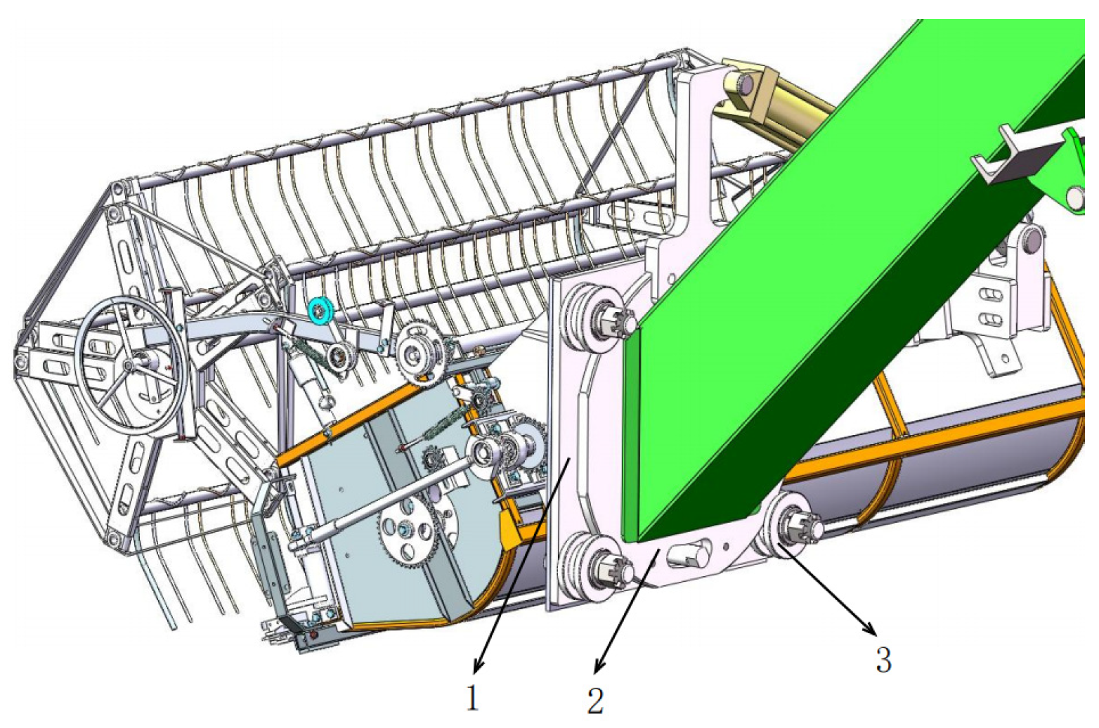
The adaptive profiling header is mainly composed of the header support frame, conveying groove, rotating disc, elevation oil cylinder, leveling oil cylinder, header, and profiling mechanism, as depicted in Figure 1a. The key parameters of the header are provided in Table 1.
The profiling mechanism mainly consists of profiling wheels, the linkage of the profiling wheel, angle sensors, four-link mechanisms, and profiling brackets, as illustrated in Figure 1b. The profiling wheel is connected to the angle sensor via a four-link mechanism and is fixed on the profiling bracket. A single profiling wheel is employed. The elevation oil cylinder is hinged with the header support frame and the conveying groove. The header is connected to the conveyor trough through a rotating disc, allowing it to swing at a specified angle through the expansion and contraction of the leveling oil cylinder. The header angle adjustment device primarily consists of a rotating disc, rotating cylinder liner, header, and connecting plate. The connecting plate is securely attached to the header, and the rotating disc, constrained by four rotating cylinder liners, closely interacts with the connecting plate, enabling the rotating of the feeding inlet at a specific angle. The leveling oil cylinder is fixedly connected to the rotating disc through a support frame. As the leveling oil cylinder expands or retracts, the rotating disc rotates around the feeding inlet, facilitating the adjustment of the header angle.
2.2. Working Principle
During operation, the profiling wheel comes into contact with the soil surface due to its own gravity. The undulations on the soil surface are then converted into the actual height of the header through an angle sensor. When the soil surface is elevated, the profiling wheel rotates clockwise with the support of the soil surface. Conversely, when the ground is sunken, the profiling wheel rotates counterclockwise. To monitor and control the header, the controller continuously gathers real-time data on the height and horizontal angle of the header through an angle sensor and an inclination sensor. These data are compared with the set value to calculate the deviation amount, which serves as the system input. The fuzzy PID control algorithm is utilized to adjust the control parameters, and the opening of the proportional valve is modified based on the voltage change after the calculation output [16]. To achieve the adaptive adjustment of the header, a three-position, four-way proportional valve is employed to control the direction and flow of the liquid. This valve drives the hydraulic cylinder to extend or shorten accordingly. The system uses PLC as the control core, angle sensor and inclination sensor input data as the control basis, and a three-position, four-way proportional solenoid valve as the actuator.
3. Key Component Design
3.1. Profiling Mechanism
The key parameters of the profiling mechanism include the length, width, and mass. The proper design of these parameters is crucial for optimum functioning. If the length of the profiling wheel linkage is excessively large, interference may occur. On the other hand, if the length is too small, it will not meet the requirements for the desired stubble height of ratooning rice. Similarly, if the width of the profiling wheel under the profiling mechanism is too narrow, it will cause the profiling wheel to sink into the soil, particularly when the soil moisture content is high, resulting in inaccurate terrain perception. Conversely, if the width is too wide, it can crush the rice stubble, affecting measurement accuracy. If the profiling wheel is heavy, it will sink into the soil, and if it is light, it will cause bouncing. According to the harvesting requirements of ratooning rice, the height of the header from the ground needs to be 300–450 mm, and the planting row spacing of ratooning rice is 25–30 mm, the length range of the profiling wheel linkage (LA) is designed to be 450–650 mm, the width range of the profiling wheel is set as 15–30 mm, and the mass range of the profile wheel is set as 2.5–5 kg.
3.2. Characterization of Header Height
The header profiling mechanism utilizes an angle sensor to measure the height of the header by measuring the angle. To investigate the angular displacement transmission relationship between the profiling mechanism and the angle sensor, a complex vector method was utilized to analyze the relative motion relationship between each member of the profiling mechanism [17].
As shown in Figure 2, the closed complex vector equation of the profiling mechanism is expressed as follows:
LRQ, LQP, LRO, LOB, and LBP are the lengths of vectors , , , , and , respectively.
Expansion is carried out according to Euler’s formula:
Elimination θ3:
The universal formula of trigonometric function is substituted into it, based on the initial position of each member of the profiling mechanism:
According to Figure 2, θ1 = θ2, the height of the header can be expressed as follows:
where WM is the total length including the profiling wheel and the profiling wheel linkage.
3.3. Analysis of Header Height Adjustment Motion
To enable the adaptive adjustment of the header, a simplified geometric model of the system was established, and force analysis was performed, as depicted in Figure 3. For automatic height adjustment, the conveying groove rotates around the hinge point by utilizing the expansion and contraction of the elevation oil cylinder, thereby causing the header to change its height. Force analysis of the model was performed, and the force at the hinge point A of the conveyor trough can be decomposed into horizontal force FAx and vertical force FAy as follows:
where yA is the vertical distance between the hinge point A and the gravity center of the soil tank test truck, mm; y is the vertical displacement of the soil tank test trolley, mm; h0 is the height from hinge point A to the ground, mm; and θ is the inclination angle of the vehicle body, (°).
Dynamic analysis was conducted:
When the force is balanced:
The height of the header can be expressed as
where lod is the projection length of lg in the vertical direction when the header is at its lowest point, m.
3.4. Analysis of Header Horizontal Adjustment Movement
The header is linked to the conveyor trough through a leveling oil cylinder and a rotating disc. The leveling oil cylinder retracts and rotates the header around the rotating disc, enabling the adjustment of the header’s angle. The motion of the header can be divided into two components: the traction motion of the soil groove test bench and the rotational motion of the header relative to the soil groove test bench. For the purpose of analysis, the traction motion is disregarded, and the motion of the header relative to the soil groove test bench is a plane rotation, as depicted in Figure 4 and Figure 5.
In the xtotytzt coordinate system, the positive direction of xt corresponds to the heading direction of the header, and the inclination sensing plane is parallel to the horizontal plane. When the header tilts to the right, the measured inclination is positive, while a leftward tilt yields a negative inclination. In the xeoeyeze coordinate system, the positive direction of xe aligns with the forward speed direction of the header. The mechanism can be simplified as the connection point between the header and the rotating hinge point, as well as the oil cylinder. Assuming a positive clockwise rotation angle of the header relative to the soil tank test bench, the elongation of the leveling oil cylinder rod l and the tilt angle of the header relative to the soil tank test bench are adjusted as follows:
where αm is the included angle oeohct, (°); βm is the angle otohcb, (°); lam is the length of ohct, mm; lbm is the length of ohcb, mm; l1 is the shortest length of the oil cylinder, mm; and l is the displacement elongation of the oil cylinder, mm.
4. MBD-DEM Coupling
In recent years, multi-body dynamics (MBD) and the discrete element method (DEM) have been widely used in agricultural engineering [18,19,20,21]. The motion of the profiling wheel incorporates the multi-body dynamics theory, while its interaction with soil involves dynamics theory and discrete element theory. As a result, the MBD-DEM coupling simulation method is used for analysis.
4.1. Multi-Body Dynamics Modeling
A multi-body dynamic model of the adaptive profiling header is established in RecurDyn. The motion pair settings between each component are outlined in Table 2; the material of all components is assumed to be steel. Additionally, a sliding pair is introduced between the header and the ground to simulate the forward movement of the harvester, with a header movement speed of 0.8 m/s. To analyze the interaction forces, marker point Ⅰ is placed at the bearing of the profiling wheel to measure the action force Y1 exerted by the header on the profiling wheel. A General Force is added between the profiling wheel and the soil to measure the action force Y2 exerted by the soil on the profiling wheel. Furthermore, marker point Ⅱ is positioned at the contact position between the profiling wheel and the soil to measure the depth of soil subsidence Y3.
4.2. Discrete Element Modeling
A soil tank model was constructed in EDEM, where soil particles were randomly generated, and the size of the soil tank was set to 2000 mm × 1000 mm × 100 mm (length × wide × height), as represented in Figure 6.
The contact model plays a crucial role in the discrete element method, and it is necessary to establish different contact models for different simulation objects. The EEPA contact model includes the plasticity and viscosity of particles, making it suitable for simulating farmland soils with strong plasticity [22]. Therefore, the EEPA contact model was chosen for the soil particle contact model. The Hertz Mindlin with JKR contact model was also selected as the contact model. According to the relevant literature [23,24], the simulation parameters of soil particles are shown in Table 3.
5. Simulation Result Analysis
5.1. The Three-Factor Quadratic Regression Orthogonal Rotational Combination Method
A three-factor quadratic regression orthogonal rotation combination experiment was conducted to investigate the impact of profiling wheel linkage length, profiling wheel width, and profiling wheel mass on the performance of the profiling mechanism. The evaluation criteria used in this experiment were the support force Y1 of the header to the profiling wheel, the support force Y2 of the soil to the profiling wheel, and the depth of soil subsidence Y3. Y1 was employed to assess whether the profiling mechanism was functioning correctly. When Y1 < 0, it indicates that the profiling wheel is off the ground, indicating a failure of the profiling mechanism. Conversely, Y1 > 0 indicates that the profiling wheel is not off the ground and the profiling mechanism is operating normally. When the profiling mechanism is operating, if the profiling wheel is not constantly rolling, but sometimes rolling and sometimes sliding, it will increase the sinking depth of the profiling wheel, making the height measurement inaccurate. The profiling wheel linkage length, profiling wheel width, and profiling wheel mass will all affect the rolling of the profiling wheel. Sensitivity is used to indicate whether the profiling wheel is rolling throughout the entire process. When Y2 is large, a larger soil force is required to force the profiling wheel to roll, indicating that the profiling wheel is not constantly rolling; the profiling mechanism is more “slow” in perceiving field terrain changes. Conversely, a lower value of Y2 indicates that the profiling mechanism is more “sensitive” in detecting terrain changes. Y3 represents the profiling accuracy of the profiling mechanism. When Y3 is small, it indicates that the soil sinks less under the action of the profiling wheel, thus indicating a higher accuracy in profiling the field terrain. The coding of experimental factors is shown in Table 4, and the simulation results are presented in Table 5.
5.2. Result Analysis
The Design-Expert 8.0.6 software was used to fit and analyze the tests and the quadratic polynomial regression models between the header support force Y1, the soil support force Y2, and the soil subsidence depth Y3. Each factor was established as presented in Equations (20)–(22):
The significance test of the regression equation is shown in Table 6. As can be seen from Table 6, the fitting degree of the above models was extremely significant (p < 0.01). At the same time, the mismatch terms were not significant (p > 0.05), indicating that the predicted values of the regression equation fit well with the actual values. There are no other major factors influencing the indicators. Hence, this regression model can be effectively utilized for analyzing and optimizing the design parameters of the profiling mechanism.
In the Y1 regression model, the primary terms X1, X2, and X3 and the secondary terms X12, X22, and X32 have a significant impact (p < 0.05). In the Y2 regression model, the primary terms X1, X2, and X3 and the secondary terms X12 and X32 have a significant impact (p < 0.05). In the Y3 regression model, the effects of primary terms X1, X2, and X3 and secondary term X12 were extremely significant (p < 0.01). To ensure that the model is significant and the mismatched items are not significant, the regression model after removing insignificant factors is expressed as follows:
Through regression coefficient testing, it was found that the primary and secondary orders of factors influencing the support force of the header on the profiling wheel are the mass of the profiling wheel, the width of the profiling wheel, and the length of the profiling wheel linkage. Similarly, the primary and secondary orders of factors affecting the soil’s support for the profiling wheel are the mass of the profiling wheel, the length of the profiling wheel linkage, and the width of the profiling wheel. In terms of the depth of soil subsidence, the primary and secondary orders of factors are the mass of the profiling wheel, the width of the profiling wheel, and the length of the profiling wheel linkage.
5.3. Response Surface Analysis
By analyzing the data using Design-Expert 8.0.6, the effects of the profiling wheel linkage length, profiling wheel width, and profiling wheel mass on Y2 could be obtained. The response surface is presented in Figure 7. To understand the interactions between the factors, a certain factor was arbitrarily fixed, and the interaction between the other two factors on Y2 was analyzed based on the response surface graph:
- (1)
- Interaction between the profiling wheel linkage length and the profiling wheel width
Figure 7a displays the response surface of the interaction between Y2 and the profiling wheel linkage length and the profiling wheel width, with a fixed mass of 3.75 kg. As shown in Figure 6, it can be observed that when the length of the profiling wheel linkage is fixed, Y2 decreases as the width of the profile wheel increases. When the width of the profiling wheel is fixed, Y2 first decreases and then increases as the length of the profiling wheel linkage increases.
- (2)
- Interaction between the length of the profiling wheel linkage and the mass of the profiling wheel
Figure 7b shows the response surface of the interaction between the length of the profiling wheel linkage and the mass of the profiling wheel and Y2 when the width of the profiling wheel is 22.5 mm. As depicted in the figure, when the length of the profiling wheel linkage is fixed, Y2 first decreases and then increases as the mass of the profiling wheel increases. Similarly, when the mass of the profiling wheel is constant, Y2 first decreases and then increases as the length of the profiling wheel linkage increases.
- (3)
- Interaction between the width of the profiling wheel and the mass of the profiling wheel
Figure 7c presents the response surface of the interaction between the width and mass of the profiling wheel and Y2 when the length of the profiling wheel linkage is 550 mm. As shown in the figure, when the width of the profiling wheel is constant, Y2 first decreases and then increases as the mass of the profiling wheel increases. Likewise, when the mass of the profiling wheel is constant, Y2 decreases as the width of the profiling wheel increases.
5.4. Optimization of Optimal Parameters
To enhance the sensitivity of the profiling mechanism in perceiving changes in terrain fluctuations, it is desirable to minimize the support force Y2 exerted by the soil on the main profiling plate. Additionally, to improve the accuracy of the profiling mechanism in detecting the height of the header, it is required to minimize the soil subsidence depth Y3 and optimize the parameters. The optimal parameters were determined as follows: profiling wheel linkage length of 562 mm, profiling wheel width of 20 mm, and profiling wheel mass of 3.6 kg. Under these parameters, the support force of the header on the profiling wheel is 47.1 N, the support force of the soil on the profiling wheel is 30.3 N, and the soil subsidence depth is 2.9 mm.
6. Control System Design
After determining the structural parameters of the adaptive profiling header, the control system was designed. Fuzzy rules were used to dynamically adjust the PID controller parameters, which can achieve the adaptive tuning of PID parameters and enhance the dynamic response ability of the system [25,26,27]. The fuzzy PID controller of the header adaptive profiling system mainly consists of an incremental PID controller and a fuzzy controller [28,29,30]. The fuzzy controller, based on fuzzy rules, is the key component of the whole controller. The fuzzy controller completes the parameter adaptive tuning through different processing, including fuzzification, fuzzy reasoning, and defuzzification. The fuzzy PID block diagram of the header adaptive profiling system is illustrated in Figure 8. The hydraulic cylinder linear displacement sensor takes the actual hydraulic rod displacement c(k) value as the actual value of the controller. It externally inputs the given values of the header height and angle r(k) to obtain the error e(k)(e(k) = r(k)−c(k)) and the change rate of the error after differentiation ∆e(k)(∆e(k) = de(k)/dt).
6.1. Fuzzy Controller Design
According to the harvesting characteristics of the ratooning rice, the feasible intervals for setting the height error e and ec of the cutting platform are [−50 cm, 50 cm] and [−10 cm/s, 10 cm/s], respectively. The feasible intervals for ∆KP are [−0.5, 0.5], ∆KI are [−0.15, 0.15], and ∆KD are [−0.2, 0.2]; the fuzzy subset quantization of input and output variables is seven levels, represented as NB, NM, NS, ZO, PS, PM, and PB; the basic domain of discourse is {−6, −5, −4, −3, −2, −1, 0, 1, 2, 3, 4, 5,6}; based on the principle of PID parameter adjustment and the actual adjustment process and experience of the height of the harvesting machine for ratooning rice, a fuzzy control rule is established, as shown in Table 7. The principle of PID parameter self-tuning is as follows:
- (1)
- When the deviation is large, to eliminate the deviation as soon as possible, improve the response speed, and avoid overshoot in the system response, it is necessary to increase KP and reduce KD, with KI usually set to zero.
- (2)
- When the deviation is small, to further reduce the deviation and prevent excessive overshoot, oscillation, and deterioration of stability, KP and KI should be increased to ensure the steady-state performance of the system.
- (3)
- When the deviation and deviation rate of change are the same sign, the controlled quantity changes in the direction of deviation from the predetermined value. Therefore, when the controlled quantity approaches a fixed value, the proportional effect of the inverse sign hinders the integral effect, avoiding integral overshoot and subsequent oscillations, which is beneficial for control.
- (4)
- When the deviation change rate is large, KP should be reduced and KI should be increased.
6.2. Fuzzy PID Control Simulation
Based on the developed system model, a fuzzy PID control simulation model is established using the Simulink simulation module in MATLAB. The step signal is employed as the system input, and the transfer functions of each link of the adaptive profiling control system are substituted into the Simulink simulation platform to construct the system simulation model, as illustrated in Figure 9.
Compared with traditional PID control, the simulation time of the system was set to 10 s. When the position of the header was adjusted from 0 to 350 mm, the simulation curve of the header response characteristics is as shown in Figure 10a. As shown in the figure, traditional PID control reaches a steady state at 4.9 s, with a maximum overshoot of 46 mm; fuzzy PID control reaches a steady state at 0.9 s. Compared with traditional PID control, the system’s rise time is reduced by 78.9%, the time required for the system to reach a steady state is reduced by 81.6%, and the system overshoot is 8.2 mm. The system stability is stronger. With any set initial angle and a simulation time of 10 s, the simulation curve of the header leveling response characteristics is as shown in Figure 10b. It can be seen that using fuzzy PID control, the system overshoot is less than 1°, and it can reach a steady state within 2.8 s. The average response speed of the header leveling to the left is about 2.38°/s, and the average response speed of the header leveling to the right is about 3.22°/s. The adjustment speed can meet the usage requirements.
7. Tests
To validate the actual effect of the adaptive profiling header, bench tests were conducted at the Zengcheng Teaching and Research Base of South China Agricultural University. The header used the 4L-1.0 II-type rice wheat combine harvester produced by Sichuan Gangyi Technology Group Co., Ltd. (SICHUAN GANGYI TECHNOLOGY GROUP, Chongzhou, China). The header was fixed to the soil tank test truck with bolts. To simulate the undulating conditions in the field, soil was collected in the field without interfering with the intact structure of the soil, it was placed on a soil tank test bench, and the height of the soil was adjusted according to the amount of soil. The travel speed of the soil tank test bench was set at 0.8 m/s, as illustrated in Figure 11.
7.1. Test Plan
The actual profiling effect of the adaptive profiling header was verified by taking the adjustment accuracy of the header, the support force of the header on the profiling wheel, the support force of the soil on the profiling wheel, and the depth of soil subsidence as indicators. The target height and angle of the header were set on the header control panel, and the automatic adjustment mode of the header was activated. The controller generated a control signal to adjust the valve opening of the three-position four-way proportional solenoid valve, thereby activating the elevation cylinder and leveling cylinder. After each experiment, ten points along the trajectory of the profiling wheel were selected at intervals of 1 m, and the depth of soil subsidence was measured using a tape measure. The average value was then calculated.
7.2. Analysis of Test Results
The adjustment accuracy serves as an important indicator for evaluating the effectiveness of the header profiling mechanism. A higher adjustment accuracy corresponds to more accurate stubble height for the first season of rice, leading to a better yield and quality of the rice during the regeneration season. The target height of the header was set in the control panel, and the displacement elongation of the oil cylinder, detected by the linear displacement sensor, served as the feedback signal of the system. The control algorithm promptly corrected the error signal to achieve the precise positioning of the header height. The actual height of the header was measured using a tape measure, and the relative error was calculated using the following formula:
where T is the set height, mm; X is the actual height of the header, mm; Za is the error amount, mm; and Eb is the relative error of height, %.
Taking the header height data measured by the angle sensor as a reference, the angle sensor output data could accurately represent the height between the header and the ground in real time. During the movement, the header height was always maintained at around 450 mm, with an average error of 6.75 mm and a maximum error of 11.63 mm. The header height control effect was good; the output angle measured by the inclination sensor was the inclination angle of the undulating road surface. The header remained horizontal throughout the movement, with an average error of 0.64° and a maximum error of 2.35°. The control effect was ideal and had a high control accuracy, indicating that the design of the profiling mechanism is reasonable and can accurately reflect the undulating conditions of the ground. The real-time data collection results are shown in Figure 12.
The values of Y1 and Y2 during the movement of the header were measured using a digital transmitter and pressure sensor, as shown in Figure 13. The average values of Y1 in the three experiments were 46.61 N, 47.26 N, and 48.63 N. It can be observed that Y1 was always greater than 0, indicating that the profiling wheel is in normal working condition during movement. The average values of Y2 were 31.98 N, 31.63 N, and 30.86 N, with similar values to the simulation results of 30.3 N, indicating reliable simulation results and a sensitive profiling wheel to the perception of ground undulation changes. The average values of soil subsidence depth Y3 were 3.4 mm, 5.6 mm, and 8.3 mm, indicating that the soil subsidence depth was relatively small during operation. The profiling wheel can accurately perceive changes in the soil surface height.
8. Discussion
Due to the inability to crush rice piles during the harvesting of ratooning rice, there is a high requirement for the grounding area of the profiling mechanism. The installation position of the profiling mechanism on the header also has a significant impact on the effectiveness of the profiling mechanism. The next step is to determine the position of the profiling mechanism on the header. Ground information is mainly collected through the four-link mechanism of the profiling mechanism. How to choose the length and installation angle of each link in the four-bar linkage mechanism to ensure the accuracy of ground information collection is also the focus of the next step of work.
9. Conclusions
- An adaptive profiling header was designed, including the profiling mechanism and control system of the header. Geometric modeling and mechanical analysis models were established. Real-time measurements of the header height were achieved through the profiling mechanism, and the height and angle of the header were adjusted by the expansion and contraction of the cylinder to achieve the adaptive leveling control of the header.
- The MBD-DEM coupling method was used to analyze the motion characteristics of the adaptive profiling header. A three-factor quadratic regression orthogonal rotation combination experiment was conducted using the profiling wheel linkage length, profiling wheel width, and profiling wheel mass as experimental factors. The results indicated that the optimal profiling effect was achieved when the profiling wheel linkage length, profiling wheel width, and profiling wheel mass were 562 mm, 20 mm, and 3.6 kg, respectively.
- The test results indicate that the header profiling mechanism can accurately perceive changes in field terrain with high profiling accuracy. It can effectively meet the harvesting and usage requirements of ratooning rice. The experimental results are basically consistent with the mathematical model and MBD-DEM coupled simulation results. That is to say, adjusting the height and horizontal angle of the header through PID fuzzy control is a feasible method. This is of great significance for further improving the yield of ratooning rice.
Author Contributions
Conceptualization, X.C.; methodology, W.L.; software, S.Z.; validation, W.L. and S.Z.; formal analysis, S.Z.; investigation, W.L.; resources, W.L.; data curation, W.L.; writing—original draft preparation, W.L.; writing—review and editing, S.Z. and X.C.; visualization, S.Z.; supervision, S.Z.; project administration, X.C.; funding acquisition, X.C. All authors have read and agreed to the published version of the manuscript.
Funding
This research was funded by the Laboratory of Lingnan Modern Agriculture Project (NT2021009) and the Jiangsu Funding Program for Excellent Postdoctoral Talent.
Institutional Review Board Statement
Not applicable.
Informed Consent Statement
Not applicable.
Data Availability Statement
The data presented in this study are available on request from the corresponding author.
Acknowledgments
The authors gratefully acknowledge the editors and anonymous reviewers for their constructive comments on our manuscript.
Conflicts of Interest
The authors declare no conflicts of interest.
References
- Zhang, M.; Wang, Z.; Luo, X.; Guo, W. Review of precision rice hill-drop drilling technology and machine for paddy. Int. J. Agric. Biol. Eng. 2018, 11, 1–11. [Google Scholar] [CrossRef]
- Wang, Y.; Zheng, C.; Xiao, S.; Sun, Y.; Huang, J.; Peng, S. Agronomic responses of ratoon rice to nitrogen management in central China. Field Crops Res. 2019, 241, 107569. [Google Scholar] [CrossRef]
- Yuan, S.; Cassman, K.; Huang, J.; Peng, S.; Grassini, P. Can ratoon cropping improve resource use efficiencies and profitability of rice in central China. Field Crops Res. 2019, 234, 66–72. [Google Scholar] [CrossRef] [PubMed]
- Wang, W.; He, A.; Jiang, G.; Sun, H.; Jiang, M.; Man, J.; Ling, X.; Cui, K.; Huang, J.; Peng, S. Ratoon rice technology: A green and resource-efficient way for rice production. Adv. Agron. 2020, 159, 135–167. [Google Scholar]
- Alizadeh, M.R.; Habibi, F. A comparative study on the quality of the main and ratoon rice crops. J. Food Qual. 2016, 39, 669–674. [Google Scholar] [CrossRef]
- Yu, X.; Yuan, S.; Tao, X. Comparisons between main and ratoon crops in resource use efficiencies, environmental impacts, and economic profits of rice ratooning system in central China. Sci. Total Environ. 2021, 799, 149–246. [Google Scholar] [CrossRef]
- Liu, W.; Luo, X.; Zeng, S.; Wen, Z.; Zeng, L. Study on field turning mechanism and performance test of crawler ratooning rice harvester. J. Jilin Univ. Eng. Technol. Ed. 2023, 53, 2659–2705. [Google Scholar]
- Ling, X.; Zhang, T.; Deng, N.; Yuan, S.; Huang, J. Modelling rice growth and grain yield in rice ratooning production system. Field Crops Res. 2019, 241, 107574. [Google Scholar] [CrossRef]
- Liu, W.; Luo, X.; Zeng, S.; Zang, Y. Numerical simulation and experiment of grain motion in the conveying system of ratooning rice harvesting machine. Int. J. Agric. Biol. Eng. 2022, 15, 103–115. [Google Scholar] [CrossRef]
- Liu, W.; Luo, X.; Zeng, S.; Zeng, L.; Wen, Z. The Design and Test of the Chassis of a Triangular Crawler-Type Ratooning Rice Harvester. Agriculture 2022, 12, 890. [Google Scholar] [CrossRef]
- Harrell, D.L.; Bond, J.A.; Blanche, S. Evaluation of main-crop stubble height on ratoon rice growth and development. Field Crops Res. 2009, 114, 396–403. [Google Scholar] [CrossRef]
- Dong, H.; Chen, Q.; Wang, W.; Peng, S.; Huang, J.; Cui, K.; Nie, L. The growth and yield of a wet-seeded rice-ratoon rice system in central China. Field Crops Res. 2017, 208, 55–59. [Google Scholar] [CrossRef]
- Tulpule, P.; Kelkar, A. Integrated robust optimal design (IROD) of header height control system for combine harvester. In Proceedings of the 2014 American Control Conference, Portland, OR, USA, 4–6 June 2014; pp. 2699–2704. [Google Scholar]
- Kassen, D.; Kelkar, A. Combine harvester header height control via robust feedback linearization. In Proceedings of the 2017 Indian Control Conference(ICC), Guwahati, India, 4–6 January 2017; pp. 1–6. [Google Scholar]
- Ni, Y.; Jin, C.; Chen, M.; Yuan, W.; Qian, Z.; Yang, T.; Cai, Z. Computational model and adjustment system of header height of soybean harvesters based on soil-machine system. Comput. Electron. Agric. 2021, 183, 105907. [Google Scholar] [CrossRef]
- Liu, W.; Luo, X.; Zeng, S.; Zeng, L. Performance test and analysis of the self-adaptive profiling header for ratooning rice based on fuzzy PID control. Trans. Chin. Soc. Agric. Eng. 2022, 38, 1–9. [Google Scholar]
- Xie, Y.; Alleyne, A.; Greer, A. Fundamental limits in combine harvester header height control. J. Dyn. Syst. Meas. Control 2013, 135, 034503. [Google Scholar] [CrossRef] [PubMed]
- Tong, Z.; Zheng, B.; Yang, Y. CFD-DEM investigation of the dispersion mechanisms in commercial dry powder inhalers. Powder Technol. 2013, 240, 19–24. [Google Scholar] [CrossRef]
- Xian, R.; Hermann, N. Simulation of particles and sediment behaviour in centrifugal field by coupling CFD and DEM. Chem. Eng. Sci. 2013, 94, 20–26. [Google Scholar]
- Ren, P.; Zhong, W.; Chen, Y. CFD-DEM simulation of spouting of corn-shaped particles. Particuology 2012, 10, 562–572. [Google Scholar] [CrossRef]
- Chu, K.; Chen, J.; Wang, B. Understand solids loading effects in a dense medium cyclone: Effect of particle size by a CFD-DEM method. Powder Technol. 2017, 320, 594–609. [Google Scholar] [CrossRef]
- Aman, M.; Mayank, K.; Narasimha, M. A coupled CFD-DEM model for tumbling mill dynamics-Effect of lifter profile. Powder Technol. 2024, 433, 119178. [Google Scholar]
- Ma, H.; Liu, Z.; Zhou, L.; Du, J.; Zhao, Y. Numerical investigation of the particle flow behaviors in a fluidized-bed drum by CFD-DEM. Powder Technol. 2023, 429, 118891. [Google Scholar] [CrossRef]
- Wang, Y.; Kang, X.; Wang, G.; Ji, W. Numerical Analysis of Friction-Filling Performance of Friction-Type Vertical Disc Precision Seed-Metering Device Based on EDEM. Agriculture 2023, 13, 2183. [Google Scholar] [CrossRef]
- Rajendiran, S.; Lakshmi, P. Simulation of PID and fuzzy logic controller for integrated seat suspension of a quarter car with driver model for different road profiles. J. Mech. Sci. Technol. 2016, 30, 4565–4570. [Google Scholar] [CrossRef]
- Yanwu, G.; Ying, H.; Xiang, D.; Meiqi, H.; Gang, L. Fuzzy-PID Speed Control of Diesel Engine Based on Load Estimation. SAE Int. J. Engines 2015, 8, 1669–1677. [Google Scholar]
- Zhu, Q.; Zhu, Z.; Zhang, H. Design of an Electronically Controlled Fertilization System for an Air-Assisted Side-Deep Fertilization Machine. Agriculture 2023, 13, 2210. [Google Scholar] [CrossRef]
- Li, C.; Wu, J.; Pan, X. Design and Experiment of a Breakpoint Continuous Spraying System for Automatic-Guidance Boom Sprayers. Agriculture 2023, 13, 2203. [Google Scholar] [CrossRef]
- Wen, S.; Zhang, Q.; Deng, J.; Lan, Y.; Yin, X.; Shan, J. Design and Experiment of a Variable Spray System for Unmanned Aerial Vehicles Based on PID and PWM Control. Appl. Sci. 2018, 8, 2482. [Google Scholar] [CrossRef]
- Xu, Y.; Gao, Z.; Khot, L.; Meng, X.; Zhang, Q. A Real-Time Weed Mapping and Precision Herbicide Spraying System for Row Crops. Sensors 2018, 18, 4245. [Google Scholar] [CrossRef]
Figure 1.
Adaptive profiling header: (1) header support frame, (2) elevation oil cylinder, (3) conveyor groove, (4) rotating disc, (5) profiling mechanism, (6) header, (7) inclination sensor, (8) leveling oil cylinder, (9) the angle sensor, (10) four-link mechanism, (11) the linkage of the profiling wheel, (12) profiling bracket. (a) The structure of the adaptive profiling header. (b) Structure of the profiling mechanism.

Figure 2.
Relative motion relationship of each member of the profiling mechanism. Note: in this article, BP is 230 mm, PB is 158 mm, and QR is 98 mm.
Figure 2.
Relative motion relationship of each member of the profiling mechanism. Note: in this article, BP is 230 mm, PB is 158 mm, and QR is 98 mm.

Figure 3.
Schematic representation of the header model. Note: S1 represents the horizontal distance between the rear wheel of the soil groove test bench and the center of gravity of the vehicle body; S2 denotes the horizontal distance between the front wheel of the soil groove test bench and the center of gravity of the vehicle body; l0 denotes the distance between the hinge point of the conveying groove and the center of gravity of the vehicle body; T represents the moment between header and body at the connection of elevation cylinder, N·m; F1 and F2 are the equivalent elastic and damping forces of the rear wheel and the front wheel, N; FAx and FAy represent the horizontal force and vertical force at the hinge joint of the conveyor, N; J1 and J2 are the rotational inertia of the rotating body and header, kg·m2; h is header height, mm; k1, k2, b1, and b2 are the elastic coefficient and damping coefficient of the front and rear wheels, respectively; Z1 and Z2 are the horizontal height of the rear wheel and front wheel, respectively, m; θ is the inclination angle of the vehicle body, (°); Φ0 is the angle between the connecting line, linking the hinge joint of the conveying trough and the gravity center of the vehicle body, and the straight line parallel to the vehicle body, (°); Φ is the angle between the hydraulic cylinder and the horizontal plane, (°); αhc is the angle between the connecting line between point a and the header center of gravity and the upper plane of the header, (°); lhc is the distance from point A to the gravity center of header, mm; α is the angle between the elevation cylinder and the conveyor, (°); β is the angle between the header upper plane and the horizontal plane, (°); la and lb are the distance from point a to the two hinge points of elevation cylinder, mm; lg denotes the length of elevation cylinder, mm; FH and FH’ represent the forces exerted by the elevation cylinder on the vehicle body and header, N; lh is the distance between the header upper plane and point A, mm; ε is the angle between two hinge points of elevation cylinder, (°); η is the angle between the header upper plane and the conveying trough, (°).

Figure 4.
Horizontal adjustment structure of the header: (1) connecting plate, (2) rotating disc, (3) rotating cylinder liner.
Figure 4.
Horizontal adjustment structure of the header: (1) connecting plate, (2) rotating disc, (3) rotating cylinder liner.

Figure 5.
Simplified diagram of the header horizontal adjustment. Note: oexeyeze corresponds to the coordinate system of the header center; otxtytzt corresponds to the coordinate system of the soil trough test trolley center; oh point is the hinge point; ot is the hinge point between the rotating mechanism and the header; Cb is the hinge point between the bottom end of the leveling cylinder and the rotating mechanism; θm is the inclination angle of the header relative to the soil trough test trolley, (°); Ct is the hinge point between the top of the leveling cylinder and the header; αm is the included angle oeohct, (°); βm is the included angle otohcb, (°); la is the length of ohct, mm; lb is the length of ohcb, mm; lt is the shortest length of the leveling cylinder rod, mm; l is the extension of the leveling cylinder rod, mm.

Figure 6.
A discrete element model: (1) soil particle bed, (2) header, (3) marker point Ⅰ, (4) marker point Ⅱ and General Force.
Figure 6.
A discrete element model: (1) soil particle bed, (2) header, (3) marker point Ⅰ, (4) marker point Ⅱ and General Force.

Figure 7.
Effects of interactive factors on the optimization index: (a) interaction between the profiling wheel linkage length and the profiling wheel width, (b) interaction between the profiling wheel linkage length and the profiling wheel mass, and (c) interaction between the profiling wheel width and the profiling wheel mass.

Figure 8.
Block diagram of fuzzy PID Controller. Note: e is the position error, mm; de is the change rate of the position error; KE and KEC are quantization factors of e and de; ∆KP, ∆KI, and ∆KD are online modification values of scale coefficient KP, integral coefficient KI, and differential coefficient KD; E and EC are the language variables of e and de.

Figure 9.
Fuzzy PID simulation model. Note: Step represents a step signal module; Integrator denotes the integration module; Derivative signifies the differential module; Fuzzy logic controller represents the fuzzy controller; Constant stands for the input constant module; Transfer Fcn denotes the transfer function; Gain represents the gain module; Add denotes the addition function; Scope signifies the oscilloscope.

Figure 10.
Response comparison experiments: (a) simulation results of the header height control based on the traditional PID and fuzzy PID and (b) fuzzy PID header leveling response diagram.
Figure 10.
Response comparison experiments: (a) simulation results of the header height control based on the traditional PID and fuzzy PID and (b) fuzzy PID header leveling response diagram.

Figure 11.
Header test: (a) side view, (b) front view. (1) Header; (2) soil tank test trolley; (3) control panel.
Figure 11.
Header test: (a) side view, (b) front view. (1) Header; (2) soil tank test trolley; (3) control panel.

Figure 12.
Test result: (a) height test and (b) header leveling test.

Figure 13.
Results: (a) first test, (b) second test, and (c) third test.


Table 1.
Main parameters of the header.
| Parameter | Value |
|---|---|
| Cutting width (mm) | 1200 |
| Header auger type | Telescopic lateral conveying |
| Reel type | Eccentric gear shifting type |
| Chopper type | Reciprocating type |
| Feeding amount (kg·s−1) | 1000 |
| Mass (kg) | 440 |
| Maximum height (mm) | 800 |
| Leveling angle range (°) | ±10 |
Table 2.
Kinematic pair configuration table of the multi-body dynamics model.
| No. | Part I | Part II | Kinematic Pair |
|---|---|---|---|
| 1 | Header | Ground | Translate |
| 2 | Header | Profiling wheel | Revolute |
| 3 | Profiling bracket | Four-link | Revolute |
| 4 | Four-link | Angle sensor | Revolute |
Table 3.
Parameter configuration table of discrete elements for soil particles.
| No. | Parameters | Value |
|---|---|---|
| 1 | Soil particle radius/mm | 5 |
| 2 | Soil particle density/(kg·m−3) | 2600 |
| 3 | Poisson’s ratio of soil particles | 0.38 |
| 4 | Static friction coefficient between soil particles | 0.6 |
| 5 | Rolling friction coefficient between soil particles | 0.26 |
| 6 | Shear modulus between soil particles/MPa | 1 |
| 7 | Recovery coefficient between soil particles | 0.37 |
| 8 | Contact adhesion energy of soil particles/J·m2 | 15.6 |
| 9 | Soil particle adhesion strength/N | −0.001 |
| 10 | Soil particle contact plasticity ratio | 0.36 |
| 11 | Soil particles–profiling wheel static friction coefficient | 0.31 |
| 12 | Soil particles–profiling wheel rolling friction coefficient | 0.13 |
| 13 | Soil particles–profiling wheel recovery coefficient | 0.54 |
| 14 | Cohesive modulus/(kN/mn+1) | 42.538 |
| 15 | Internal friction modulus/(kN/mn+2) | 9.004 |
| 16 | Soil deformation index | 0.8227 |
| 17 | Soil moisture content/% | 37.3 |
| 18 | Soil compaction/kPa | 3093.5 |
Table 4.
Coding of factors and levels.
| Code | Length of Profiling Wheel Linkage (mm) | Width of Profiling Wheel (mm) | Profiling Wheel Mass (kg) |
|---|---|---|---|
| −1.682 | 450 | 15 | 2.5 |
| −1 | 490.54 | 18.04 | 3.01 |
| 0 | 550 | 22.5 | 3.75 |
| 1 | 609.46 | 26.96 | 4.49 |
| 1.682 | 650 | 30 | 5 |
Table 5.
Simulation result.
| No. | Parameters | Value | ||||
|---|---|---|---|---|---|---|
| Length of Profiling Wheel Linkage X1 (mm) | Width of Profiling Wheel X2 (mm) | Profiling Wheel Mass X3 (kg) | Y1 | Y2 | Y3 | |
| 1 | −1 | −1 | −1 | 44.9 | 38 | 6.5 |
| 2 | 1 | −1 | −1 | 45.7 | 68 | 1.8 |
| 3 | −1 | 1 | −1 | 44.6 | 28 | 7.9 |
| 4 | 1 | 1 | −1 | 45.6 | 32 | 5.6 |
| 5 | −1 | −1 | 1 | 44.5 | 65 | 4.4 |
| 6 | 1 | −1 | 1 | 45.8 | 72 | 1.2 |
| 7 | −1 | 1 | 1 | 43.6 | 47 | 8.1 |
| 8 | 1 | 1 | 1 | 44.9 | 49 | 5.3 |
| 9 | −1.682 | 0 | 0 | 44.0 | 25 | 9.4 |
| 10 | 1.682 | 0 | 0 | 45.1 | 83 | 1.5 |
| 11 | 0 | −1.682 | 0 | 47.1 | 38 | 1.9 |
| 12 | 0 | 1.682 | 0 | 45.2 | 21 | 7.5 |
| 13 | 0 | 0 | −1.682 | 46.1 | 22 | 5.6 |
| 14 | 0 | 0 | 1.682 | 44.6 | 87 | 2.0 |
| 15 | 0 | 0 | 0 | 46.7 | 27 | 3.8 |
| 16 | 0 | 0 | 0 | 46.3 | 29 | 4.4 |
| 17 | 0 | 0 | 0 | 47.1 | 15 | 4.3 |
| 18 | 0 | 0 | 0 | 46.7 | 25 | 4.0 |
| 19 | 0 | 0 | 0 | 47.3 | 16 | 3.8 |
| 20 | 0 | 0 | 0 | 46.7 | 34 | 3.2 |
| 21 | 0 | 0 | 0 | 46.6 | 39 | 2.9 |
| 22 | 0 | 0 | 0 | 46.8 | 26 | 3.7 |
| 23 | 0 | 0 | 0 | 47 | 28 | 3.2 |
Table 6.
Variance analysis of regression equation.
| Variance Source | The Header Support Force Y1 | The Soil Support Force Y2 | The Soil Subsidence Depth Y3 | |||||||||
|---|---|---|---|---|---|---|---|---|---|---|---|---|
| Square Sum | Degree of Freedom | F | p | Square Sum | Degree of Freedom | F | p | Square Sum | Degree of Freedom | F | p | |
| Model | 21.45 | 9 | 15.82 | <0.0001 ** | 8145.21 | 9 | 6.80 | 0.0030 ** | 102.10 | 9 | 20.96 | <0.0001 ** |
| X1 | 2.86 | 1 | 18.99 | 0.0014 ** | 1446.35 | 1 | 10.86 | 0.0081 ** | 50.59 | 1 | 93.46 | <0.0001 ** |
| X2 | 2.13 | 1 | 14.15 | 0.0037 ** | 978.35 | 1 | 7.35 | 0.0129 * | 36.80 | 1 | 67.98 | <0.0001 ** |
| X3 | 1.50 | 1 | 9.94 | 0.0103 * | 2276.33 | 1 | 17.09 | 0.0020 ** | 5.74 | 1 | 10.60 | 0.0086 ** |
| X1X2 | 0.005 | 1 | 0.033 | 0.8591 | 120.13 | 1 | 0.90 | 0.3646 | 0.98 | 1 | 1.81 | 0.2082 |
| X1X3 | 0.080 | 1 | 0.53 | 0.4829 | 78.13 | 1 | 0.59 | 0.4614 | 0.13 | 1 | 0.23 | 0.6412 |
| X2X3 | 0.24 | 1 | 1.63 | 0.2310 | 3.13 | 1 | 0.023 | 0.8813 | 0.84 | 1 | 1.56 | 0.2400 |
| X12 | 10.69 | 1 | 70.98 | <0.0001 ** | 1753.01 | 1 | 13.16 | 0.0046 ** | 5.68 | 1 | 10.49 | 0.0089 ** |
| X22 | 1.26 | 1 | 8.36 | 0.0161 * | 80.75 | 1 | 0.61 | 0.4542 | 1.89 | 1 | 3.50 | 0.0909 |
| X32 | 4.82 | 1 | 32.02 | 0.0002 ** | 1809.66 | 1 | 13.59 | 0.0042 ** | 0.028 | 1 | 0.052 | 0.8237 |
| Residual | 1.51 | 10 | 1331.74 | 10 | 5.41 | 10 | ||||||
| Lack of fit | 0.89 | 5 | 1.43 | 0.3522 | 1052.41 | 5 | 3.77 | 0.0859 | 4.49 | 5 | 4.83 | 0.0544 |
| Error | 0.62 | 5 | 279.33 | 5 | 0.93 | 5 | ||||||
| Sum | 22.96 | 19 | 9476.95 | 19 | 107.52 | 19 | ||||||
Note: * significant (p < 0.05) and ** extremely significant (p < 0.01).
Table 7.
Fuzzy rule table.
| Parameters | ec | e | ||||||
|---|---|---|---|---|---|---|---|---|
| NB | NM | NS | ZO | PS | PM | PB | ||
| NB | PB | PB | PM | PM | PS | ZO | ZO | |
| NM | PB | PB | PM | PS | PS | ZO | NS | |
| NS | PM | PM | PM | PS | ZO | NS | NS | |
| KP | ZO | PM | PM | PS | ZO | NS | NM | NM |
| PS | PS | PS | ZO | NS | NM | NM | NM | |
| PM | PS | ZO | NS | NM | NM | NM | NB | |
| PB | ZO | ZO | NM | NM | NB | NB | NB | |
| NB | NB | NB | NM | NM | NS | ZO | ZO | |
| NM | NB | NB | NM | NS | NS | ZO | ZO | |
| NS | NB | NM | NS | NS | ZO | PS | PS | |
| KI | ZO | NM | NM | NS | ZO | PS | PM | PM |
| PS | NM | NS | ZO | PS | PS | PM | PB | |
| PM | ZO | ZO | PS | PS | PM | PB | PB | |
| PB | ZO | ZO | PS | PM | PM | PB | PB | |
| NB | PS | NS | NB | NB | NB | NM | PS | |
| NM | PS | NS | NB | NM | NM | NS | ZO | |
| NS | ZO | NS | NM | NM | NS | NS | ZO | |
| KD | ZO | ZO | NS | NS | NS | NS | NM | ZO |
| PS | ZO | ZO | ZO | ZO | ZO | ZO | ZO | |
| PM | PB | NS | PS | PS | PS | PS | PB | |
| PB | PB | PM | PM | PM | PS | PS | PB | |
Disclaimer/Publisher’s Note: The statements, opinions and data contained in all publications are solely those of the individual author(s) and contributor(s) and not of MDPI and/or the editor(s). MDPI and/or the editor(s) disclaim responsibility for any injury to people or property resulting from any ideas, methods, instructions or products referred to in the content. |
© 2024 by the authors. Licensee MDPI, Basel, Switzerland. This article is an open access article distributed under the terms and conditions of the Creative Commons Attribution (CC BY) license (https://creativecommons.org/licenses/by/4.0/).
Share and Cite
MDPI and ACS Style
Liu, W.; Zeng, S.; Chen, X. Design and Experiment of Adaptive Profiling Header Based on Multi-Body Dynamics–Discrete Element Method Coupling. Agriculture 2024, 14, 105. https://doi.org/10.3390/agriculture14010105
AMA Style
Liu W, Zeng S, Chen X. Design and Experiment of Adaptive Profiling Header Based on Multi-Body Dynamics–Discrete Element Method Coupling. Agriculture. 2024; 14(1):105. https://doi.org/10.3390/agriculture14010105
Chicago/Turabian StyleLiu, Weijian, Shan Zeng, and Xuegeng Chen. 2024. "Design and Experiment of Adaptive Profiling Header Based on Multi-Body Dynamics–Discrete Element Method Coupling" Agriculture 14, no. 1: 105. https://doi.org/10.3390/agriculture14010105
Note that from the first issue of 2016, this journal uses article numbers instead of page numbers. See further details here.