Article

Effects of Recurrent Selection on Population Structure and Allele Frequencies in the M3S Maize Population

1
Department of Plant Breeding, Genetics and Biometrics, Faculty of Agriculture, University of Zagreb, Svetošimunska cesta 25, 10000 Zagreb, Croatia
2
Department of Plant Breeding, Genetics, Seed Production and Biometrics, Faculty of Agriculture and Food Technology, University of Mostar, Biskupa Čule bb, 88000 Mostar, Bosnia and Herzegovina
3
Department of Crop and Soil Science, North Carolina State University, Campus Box 7620, Raleigh, NC 27695, USA
4
Centre of Excellence for Biodiversity and Molecular Plant Breeding (CroP-BioDiv), Svetošimunska cesta 25, 10000 Zagreb, Croatia
5
Department of Maize Breeding and Genetics, Agricultural Institute Osijek, Južno predgrađe 17, 31000 Osijek, Croatia
*
Author to whom correspondence should be addressed.
Agriculture 2024, 14(1), 49; https://doi.org/10.3390/agriculture14010049
Submission received: 25 November 2023 / Revised: 21 December 2023 / Accepted: 25 December 2023 / Published: 27 December 2023

Abstract

:
The effects of four cycles of recurrent selection on the allele frequencies of simple sequence repeat (SSR) markers and population structure were examined in the Maksimir 3 Synthetic (M3S) maize population (Zea mays L.). Genotyping of 32 plants from each selection cycle at 38 SSR loci revealed that the mean number of alleles per locus and the mean expected heterozygosity were preserved across selection cycles, indicating the maintenance of sufficient genetic variability in the population required for future genetic gain. The Waples test of selective neutrality revealed that genetic drift was the main force in changing allele frequencies in the population. The proportion of selectively non-neutral loci in single cycles of selection varied between 16% and 37%. Some non-neutral loci shared the same genomic locations with previously published QTLs controlling important agronomic traits. An analysis of molecular variance revealed that 5.6% of the genetic variation occurred among and 94.4% within cycle populations. Between 5% and 29% of loci were found to be in a significant Hardy–Weinberg (HW) disequilibrium, with the majority showing an excess of homozygosity. The excess of homozygosity at several loci was highly consistent across cycle populations, suggesting positive assortative mating as a possible cause of the observed HW disequilibrium. Linkage disequilibrium (LD) tests revealed that the M3S population was essentially in linkage equilibrium. The proportion of pairs of loci in significant LD varied from 0.1% to 1.8% across selection cycles, probably due to the effects of genetic drift and epistatic selection.

1. Introduction

A broad class of selection methods referred to as recurrent selection (RS) uses a cyclical approach to gradually increase the frequency of favorable alleles affecting quantitatively inherited traits in broad-based plant populations while maintaining genetic variability for future selection [1]. The two primary forces affecting allele frequencies in RS programs are selection, which increases the frequency of favorable alleles, and genetic drift, which is a random change in allele frequency due to small population sizes [2]. An expected effect of random genetic drift in a population is the dispersion of allele frequencies from intermediate values toward the extremes [3], a phenomenon that has been observed in maize populations under RS [4,5,6,7]. Problems associated with finite population sizes, such as the fixation of undesirable alleles due to random genetic drift, affect the response to selection [8], implying a trade-off between short-term selection favored by higher intensities and long-term selection favored by higher effective population sizes [9]. A relevant question is the extent to which selection influences allele frequencies in a population subjected to recurrent selection. A number of studies have reported significant changes in allele frequencies at isozyme, RFLP, SSR, and SNP marker loci due to selection [2,4,5,6,7,8,9,10,11,12,13,14,15,16,17]. Falke et al. [2], Coque and Gallais [12], and Wisser et al. [13] identified marker loci, whose allele frequencies were significantly changed by selection, to reside in genomic regions where QTLs affecting important maize agronomical traits of maize had previously been identified. The observed correlation between allele frequency changes at markers linked to QTLs and phenotypic performance suggested the possibility of using these markers in marker-assisted breeding programs [2,12]. In addition to information on alleles subjected to selection, the extent of genetic diversity in improved selection cycles is also important information for breeders because the future response of the population to selection depends on it. Several studies have reported a significant decrease in genetic diversity as measured by the number of marker alleles per locus and expected heterozygosity (gene diversity) in populations subjected to RS [7,14,18,19,20,21,22]. On the other hand, Kolawole et al. [17] reported that the changes in the different measures of genetic diversity due to selection in two maize composites were either small or negligible.
RS methods were developed to gradually improve the mean performance of genetically broad-based populations, and their incorporation in current breeding programs could facilitate the use of exotic germplasm [23] as well as locally adapted but non-improved germplasm [24] to increase the genetic base of maize breeding germplasm. Several researchers around the world, aware of the danger posed by the loss of genetic variability associated with the abandonment of landraces, made efforts to collect them before their total disappearance [25]. With the aim to exploit genetic variability existing in locally adapted maize germplasm from Southeast Europe, a synthetic maize population named Maksimir 3 Synthetic (M3S) was developed at the Faculty of Agriculture, University of Zagreb (Croatia) by intercrossing 12 inbred lines originating from locally adapted open-pollinated varieties and landraces from different regions of former Yugoslavia [26]. The 12 M3S progenitor lines showed equally good combining ability for grain yield with both the BSSS and Lancaster testers [27] and the same level of isoenzymic differences to both testers [28]. After its creation, M3S was subjected to four cycles of intrapopulation RS primarily for grain yield, but the resistance to leaf and stalk diseases was also considered [26,29,30,31]. After two selection cycles, grain yield increased slightly in the population per se, but the selection was more effective in reducing inbreeding depression for grain yield [26]. After the third cycle of selection, Sabljo et al. [29] observed no further improvement in grain yield, but stalk rot incidence significantly decreased. In the fourth cycle of selection, performed under low and high N conditions (0 and 150 kg N ha−1, respectively), Bukan et al. [30] found an indication of the specific adaptation of the two C4 populations to contrasting N environments. The resulting C4N0 population, which has been developed by intercrossing individuals selected in a low N environment, showed a significant reduction in ASI, which is typical for the genetic material more suited to low N environments. Although no significant yield increase was observed from C3 to C4, both resulting C4 populations (C4N0 and C4N150) performed well in their target N fertilization environments. Also, after applying RS methods, the resistance to stalk rot diseases in the M3S population appeared to be maintained [31].
Šarčević et al. [6] examined changes in allele frequencies at nine SSR loci in the M3S maize population after two cycles of RS and found significant changes in allele frequencies at four loci. In some previous studies, including Šarčević et al. [6], genetic changes in populations under RS were assessed by comparing the starting (base) populations and the advanced populations developed through a certain number of selection cycles. However, according to Coque and Gallais [12], the main problem to solve when studying more than one selection cycle is to test whether allelic frequency changes are due to selection or genetic drift. To obtain a better insight into the genetic changes of a population under RS, it would be useful to monitor the effects of selection at the molecular level from cycle to cycle. In the present study, we examined the M3S maize population at the molecular level after four cycles of RS by monitoring the selection response in each single cycle of selection using 38 SSR markers. The objectives of the study were (1) to investigate changes in allele frequencies in the population due to the effects of random genetic drift and selection and (2) to investigate population structure concerning the partitioning of genetic variation among and within cycle populations and concerning the Hardy–Weinberg (HW) disequilibrium at individual loci and linkage disequilibrium (LD) between pairs of loci within cycle populations.

2. Materials and Methods

2.1. Development of M3S Cycle Populations

The Maksimir 3 Synthetic (M3S) cycle 0 population (C0) was developed by intermating 12 maize inbred lines, whose origin traces back to several landraces and open-pollinated varieties from different regions of former Yugoslavia [26]. Four cycles of intrapopulation recurrent selection (RS), primarily for grain yield, were conducted in the M3S (Figure 1, Table S1).
In the first cycle, two-stage S1-S2 selection was performed with emphasis on disease resistance (Setosphaeria turcica and Colletotrichum graminicola (Ces) GW Wils) among S1 progenies and grain yield among S2 progenies resulting in the C1 population. In the second cycle, selection for higher grain yield was conducted among S1 progenies, resulting in the C2 population. In the third cycle, two selection methods, including evaluation of S1 and full-sib (FS) progenies, were conducted simultaneously to improve grain yield, resulting in two C3 populations, C3S1 and C3FS, respectively. The low response to selection observed in the C3S1 population [29] led to the fourth cycle of selection starting from the C3FS population, in which S1 progenies were evaluated simultaneously at low nitrogen fertilization (0 kg N ha−1) and high nitrogen fertilization (150 kg N ha−1), resulting in two C4 populations, C4N0 and C4N150, respectively. Details of the experimental procedures used in population synthesis and the four selection cycles have been described previously [26,29,30,31].

2.2. Simple Sequence Repeat (SSR) Genotyping

Thirty-two plants randomly selected from each of the C0, C1, C2, C3S1, C3FS, C4N0, and C4N150 cycle populations of M3S were grown in a growth chamber. After about three weeks, DNA was extracted from each plant using a GenElute Plant Genomic DNA Miniprep Kit (Sigma-Aldrich, St. Louis, MO, USA). Forty SSR primer pairs were chosen for analysis on the basis of previous polymorphism identification in M3S [6] and based on genomic location in order to provide a uniform coverage of all ten maize chromosomes. After an initial analysis, two markers were discarded because of poor amplification. Primer pairs were fluorescently labeled prior to polymerase chain reactions (PCRs). PCRs were performed in 15 μL final volumes containing 25 ng of template DNA, a 1× PCR buffer with added 1.5 mM MgCl2, 0.2 μM of each of the forward and reverse primers, 0.2 mM of dNTPs, and 0.5 U of Taq polymerase (Sigma-Aldrich, St. Louis, MO, USA). Reactions were carried out on a Veriti 96-Well Fast Thermal Cycler (Applied Biosystems, Foster City, CA, USA). Reactions were denatured at 95 °C for 2 min, followed by 30 cycles of 92 °C for 1 min, 55 °C for 1 min, and 72 °C for 2 min. This was followed by a final extension step at 72 °C for 10 min. Diluted PCR products (in ddH20) were mixed with 8.75 μL HiDi (Applied Biosystems, Foster City, CA, USA) and 0.25 μL Genescan 500 LIZ size standard (Applied Biosystems, Foster City, CA, USA), centrifuged, denatured at 95 °C for 5 min, and placed on ice. Fragment analysis was performed using an ABI 3130 Genetic Analyzer (Applied Biosystems, Foster City, CA, USA). GeneMapper 4.0 software (Applied Biosystems, Foster City, CA, USA) with the sizing algorithm “2nd order least square” was used to detect allele sizes.

2.3. Statistical Analysis of the SSR Data

2.3.1. Diversity Statistics and Allele Frequency

For each cycle population, the total number of SSR alleles (At), the mean number of alleles per locus (Am), the observed heterozygosity (Ho), and the expected heterozygosity (He) were calculated. Allele frequencies were estimated using the software package Genealex 6 [32]. The Waples test of temporal variation in allele frequency [33] was used to test the selective neutrality of alleles at 38 SSR loci from cycle to cycle, as well as after four cycles of selection. The Waples method tests the hypothesis that observed differences in allele frequency can be explained entirely by sampling processes, both in choosing gametes to form the next generations (genetic drift) and in choosing the sample for genetic analysis (sampling error). Loci with one or more non-neutral alleles (rejecting the null hypothesis of the Waples test) were designated as non-neutral loci. The effective population size (Ne) for the particular cycle of selection was assumed to be equal to the number of intermated progenies (N) in that cycle. Because S2 progenies were intermated in the first cycle of selection, Ne for the first cycle of selection was corrected by multiplying N with the term 1/(1 + Fp), where Fp = 0.5 is the inbreeding coefficient of the parental generation (S1) from which the S2 progenies were produced [34]. The Ne after four selection cycles was calculated as the harmonic mean of the Ne values from individual selection cycles [3].

2.3.2. Population Structure

Wright’s fixation index was estimated using the formula FIS = 1 − (Ho/He) to quantify the lack or excess of heterozygosity. Significant deviations from the Hardy–Weinberg (HW) equilibrium at individual loci were determined using the likelihood ratio G test [35]. The significance of linkage disequilibrium (LD) between pairs of alleles from different loci was determined using the χ2 test outlined by Weir [36]. The calculations of Ho, He, and FIS, as well as the HW equilibrium and LD tests, were performed using the software package Popgene 1.31 [37].
To compare the observed proportions of pairs of loci in a significant LD involving linked vs. unlinked loci, as well as non-neutral vs. neutral loci (based on the Waples neutrality test) in a particular cycle population, we derived two equations (Equations (1) and (2)). The probability that the two randomly selected loci are linked P l l was calculated as the number of possible pairs involving linked loci relative to the number of possible pairs involving all loci (Equation (1)):
P l l = i = 1 10   n i n i 1 N N 1
where n i is the number of loci at the i-th chromosome, and N is the total number of loci. The probability that the two randomly selected loci are non-neutral P n n l was calculated as the ratio of the number of possible pairs of non-neutral loci and the number of possible pairs of all loci (Equation (2)):
P n n l = n n n l   n n n l 1 N N 1
where n n n l is the number of non-neutral loci, and N is the total number of loci. The derivation of Equations (1) and (2) is shown in Appendix A.
In order to detect differences in the distribution of multilocus genotypes among and within the cycles of selection, we performed an analysis of molecular variance (AMOVA) [38] using Arlequin 3.5 [39]. The sources of variation included seven cycle populations (C0, C1, C2, C3S1, C3FS, C4N0, and C4N150) and 224 plants representing the entire sample. The pairwise fixation index, ΦST, provides an indication of the genetic distance between cycle populations [12]. The significance of the average fixation index, as well as of each pairwise ΦST value, was obtained after 1023 permutations.

3. Results

3.1. Diversity Statistics and Allele Frequency

The 38 SSR primer pairs generated a total of 133 different alleles (an average of 3.5 alleles per locus) across seven M3S cycle populations. The number of alleles per locus varied from two to seven. The total number of alleles (At) for individual cycle populations varied from 123 (mean of 3.2 alleles per locus) found for C3FS to 130 (mean of 3.4 alleles per locus) found for C1 and C2, although the differences were not significant (Table 1). Mean expected heterozygosity (He) ranged from 0.49 in C4N150 to 0.53 in C1 but observed differences among cycle populations were not found to be significant. Six alleles found in advanced cycle populations were not found in the original base population (C0). Seventeen alleles from 13 loci that were present in C0 were absent from one or more improved cycle populations. Most of these alleles in the base population were found in low frequencies (less than 0.10).
Mean allele frequencies remained unchanged (0.29 ± 0.02) after four cycles of selection, but the shape of the frequency distribution changed slightly (Table 2). Generally, slightly higher percentages of alleles with low (≤0.10) and high (>0.80) frequencies were observed in improved cycle populations relative to the base population.
The number of non-neutral loci detected by the Waples test varied among single cycles of selection from six (as found between C2 and C3S1) to 14 (as found between C2 and C3FS) (Table 3). In the fourth cycle of selection, more non-neutral loci were found for C4N150 than for C4N0 (nine vs. seven). However, the cumulative changes in allele frequency over four selection cycles resulted in a higher number of non-neutral loci for C4N0 (six) than for C4N150 (three). Considering single cycles of selection, non-neutral loci were found on all ten maize chromosomes, with the lowest incidence on chromosome 6 (four cases) and the highest incidence on chromosome 1 (nine cases). The occurrence of non-neutral loci was inconsistent across cycles of selection, but discrepancies were also observed between the neutrality status of loci after four cycles of selection and their neutrality status across individual cycles of selection. Of the 38 loci, 28 were non-neutral in at least one single cycle, 5 were non-neutral across three cycles, and none of them were non-neutral across all four cycles of selection. Even in cases where a particular marker locus was recognized as non-neutral over several cycles of selection, there was inconsistency in the neutrality status of different alleles at these loci (Table S2).

3.2. Analysis of Molecular Variance (AMOVA)

Analysis of molecular variance revealed that 5.6% of the genetic variation occurred among and 94.4% within M3S cycle populations. The average fixation index, ΦST, commonly used to estimate the extent of differentiation in population subdivisions [19], was 0.0559. The pairwise ΦST values between cycle populations, interpreted here as the genetic distance between them, were all significant (Table 4).
The highest ΦST was observed between C1 and C3FS (0.0872), followed by ΦST observed between C1 and C4N150 (0.0843). The lowest ΦST values were determined between C2 and C3S1 and between C4N0 and C4N150 (0.0143). The highest mean ΦST value of a cycle population to the remaining cycle populations was observed for C1.

3.3. Hardy–Weinberg (HW) Disequilibrium

The number of loci that were not in the HW equilibrium varied across M3S cycle populations from 2 (5%), observed in C3FS, to 11 (29%), observed in C3S1 (Figure 2). Most of them showed an excess of homozygotes.
In total, 26 SSR loci (68%) were identified to be in significant HW disequilibrium in at least one cycle population, and such loci were found on all chromosomes except chromosome 3 (Table S3). Fixation indices (FIS) for six loci, which were not in HW equilibrium in three or more of the cycle populations, are shown in Table 5. Two of these loci (bnlg143 and phi050) showed a significant excess of homozygosity (positive FIS value) in five and one locus (bnlg572) in six of seven cycle populations. All six loci had a positive FIS, averaged over populations, with the highest value observed for the locus bnlg572 (0.65).

3.4. Linkage Disequilibrium (LD)

In the base population (C0), 3 (0.4%) out of 703 possible pairs of loci were in significant LD (Table 6). The number of significant LD tests in the improved cycle populations varied from only 1 (0.1%) in C3S1 to 13 (1.8%) in C1. Out of three pairs of loci found to be in significant LD in C0, only one pair (which included two linked loci on chromosome 8) was found to be later in LD (in C3FS). Besides this pair, eight cases of newly generated LD between linked loci were found in the improved cycle populations. However, the majority of the newly generated LD involved unlinked loci. The proportions of marker pairs in LD across cycle populations involving linked loci were 0.33 (C0), 0.23 (C1), 0.00 (C2), 1.00 (C3S1), 0.43 (C3FS), 0.40 (C4N0), and 0.25 (C4N150), which is in most cases more than three times higher than the probability that the two randomly selected loci were linked (0.08, according to Equation (1)).
Some loci were found more frequently to be in significant LD, like bnlg197 and phi015 (in five and four out of seven cycle populations, respectively), but there were only three pairs of loci in significant LD, which were found at the same time in two or more improved cycle populations (dupssr12 and phi015 in C1 and C4N0; bnlg197 and dupssr12 in C1, C2, and C4N150; and bnlg128 and phi033 in C1 and C3FS). Most pairs of loci found to be in significant LD in improved cycle populations included one or both non-neutral loci (according to the Waples neutrality test). The observed proportion of LD pairs, including both non-neutral loci, was at least three times higher than expected (according to Equation (2)) in four out of five improved cycle populations (C3S1 was not considered because only one test was significant) with the observed to expected ratio being 0.31:0.11, 0.25:0.08, 0.43:0.13, 0.00:0.03, and 0.50:0.05 for C1, C2, C3FS, C4N0, and C4N150, respectively.

4. Discussion

4.1. Diversity Statistics and Allele Frequency

In the present study, the effects of four cycles of recurrent selection on the allele frequencies of simple sequence repeat (SSR) markers and population structure of the Maksimir 3 Synthetic (M3S) maize population were examined. The variability of the C0 population, in terms of the mean number of alleles per locus and expected heterozygosity, was in the order of magnitude of the starting population of other RS programs [5,7,9,14,19].
The mean number of alleles per locus and the mean expected heterozygosity did not change significantly in the M3S population after four cycles of RS. Similarly, in the study of Wisser et al. [40], neither of the two diversity measures, determined by SSR markers, changed significantly after four cycles of RS for quantitative disease resistance in a complex maize population from CIMMYT. Kolawole et al. [17] and Wisser et al. [40] reported that the changes in different measures of SNP diversity were either small or negligible in maize populations subjected to recurrent selection. In the study by Daas et al. [41], the genetic diversity of the two maize populations also did not change significantly after two cycles of genomic selection. In contrast, Labate et al. [18] and Hinze et al. [19] observed a significant decrease in the mean number of alleles per locus and expected heterozygosity in the BSSS and BSCB1 populations after 12 and 15 cycles of reciprocal RS, respectively. A decrease in marker diversity (in terms of the number of polymorphic loci, mean number of alleles per locus, expected heterozygosity, or observed heterozygosity) within maize populations that underwent various numbers of RS cycles has also been reported in several previous studies [7,14,20,21,22,42,43,44,45,46,47].
In the present study, some alleles found in the base population (C0) were absent from subsequent cycle populations, while some alleles absent from the base population were detected in one or more subsequent cycle populations. Most of the missing alleles were generally found at low frequencies (less than 0.10), similar to the study of McLean-Rodríguez et al. [48], where most of the alleles lost or gained over time in 13 Mexican landraces had rare or low frequencies. Such rare alleles may not have been detected in the particular cycle population in the present study because of the relatively small sample size (32 plants per cycle population genotyped), which was also the case in the study by McLean-Rodriguez et al. [48], who sampled only 10 plants per population. Nevertheless, our sample size is comparable to the sample size of 30 plants used for the SSR analysis of the BSSS and BSCB1 populations studied by Hinze et al. [19]. In an earlier study, Labate et al. [18] genotyped 100 individuals from the same two maize populations using RFLP markers and reported higher estimates of average number of alleles per locus, expected heterozygosity, heterozygous plants, and number of unique alleles, which reflects not only the differences between the two types of markers used in the two studies (RFLPs versus SSRs), but also the power of larger sample sizes in detecting less frequent alleles [19]. Although the sample size of 32 genotyped plants per population in the present study was relatively small, it is comparable to sample sizes reported in some previous studies in maize using SSR markers [17,18] as well as SNP markers [19,20,48], which ranged from 10 to 36 individuals per population. However, the possible role of pollen or seed contamination during the development of the M3S cycle populations cannot be excluded either.
In improved M3S cycle populations compared to C0, the mean allele frequency did not change, although slightly higher proportions of alleles with low and high frequencies were found. Similar changes in allele distribution after various cycles of RS in maize have been earlier found by Labate et al. [4], Pinto et al. [5], and Šarčević et al. [6], whereas Kolawole et al. [17] reported the opposite, a decrease in the proportion of alleles at both low and high frequencies and an increase in those at intermediate frequencies.
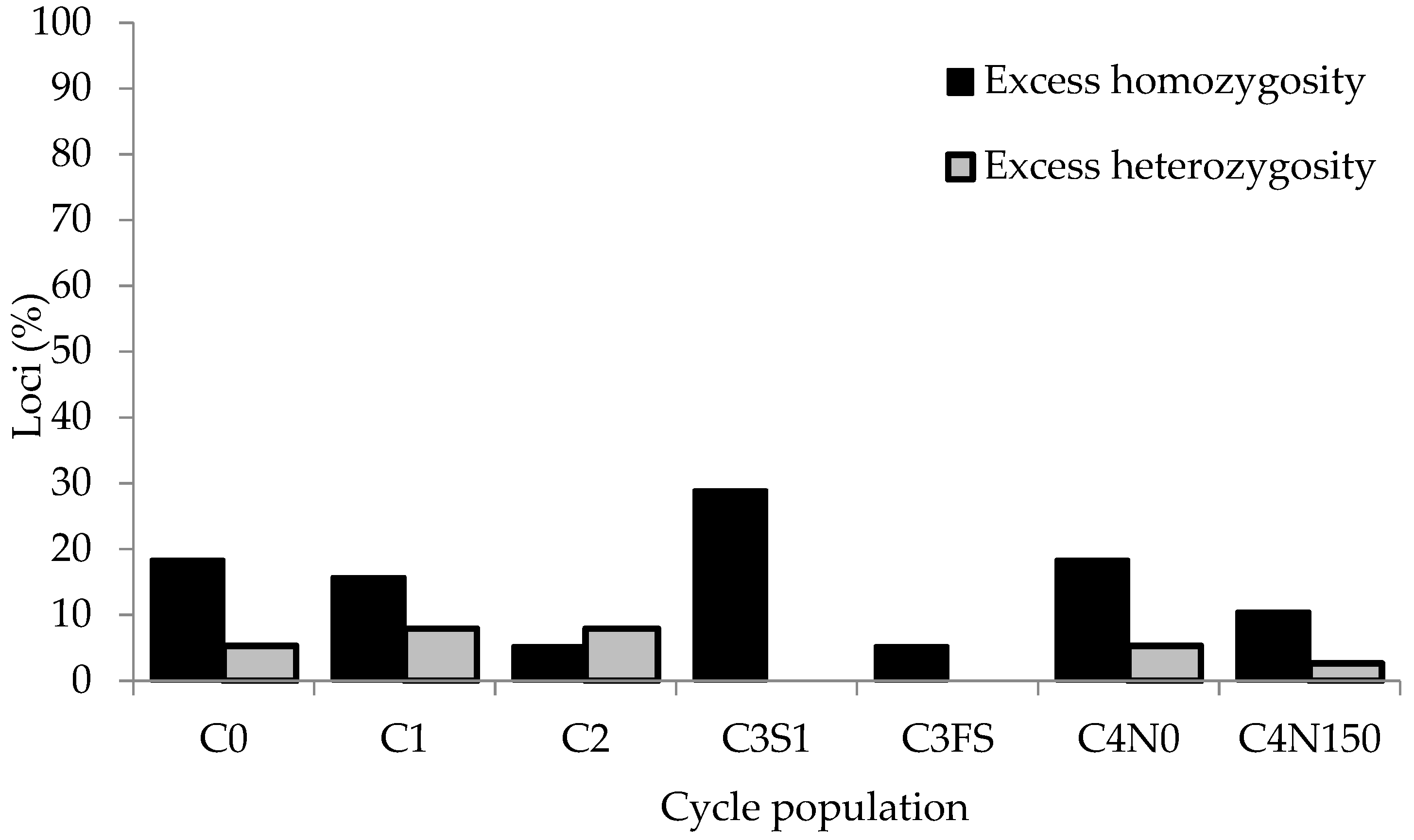
The changes in allele frequencies from cycle to cycle as well as after four cycles of selection in M3S as determined by the Waples test, were mainly attributable to the effects of random genetic drift. Similar results were reported in previous studies examining changes in allele frequencies in maize populations subjected to RS [2,4,5,43]. Assuming the value of Ne = N, the Waples test identified six (16%) and three (8%) non-neutral loci after four cycles of selection from C0 to C4N0 and C4N150, respectively (Table 3). The number of non-neutral loci in single cycles varied between 6 (16%), as found between C2 and C3S1, and 14 (37%), as found between C2 and C3FS. Labate et al. [4] observed 17% non-neutral loci in BSSS(R) and BSCB1(R) populations after 12 cycles of reciprocal RS. Pinto et al. [5] reported significant changes in allele frequency due to selection at 13% and 7% of SSR loci in two tropical maize synthetics subjected to a single cycle of high-intensity reciprocal RS. Falke et al. [2] detected 20.13% non-neutral loci in one and 12.87% in a second biparental maize population after four and seven cycles of intrapopulation RS, respectively. In these studies, loci with significant changes in allele frequency due to selection were not restricted to particular chromosomes or genomic regions but were scattered throughout the genome. In our study, selectively non-neutral loci were also found on all ten maize chromosomes, but their number and chromosomal position varied among cycles of selection. The occurrence of non-neutral loci was inconsistent across the four selection cycles, but discrepancies were also observed between the neutrality status of loci after four cycles of selection and their neutrality status across individual cycles of selection (Table S2). Even in cases where a particular marker locus was recognized as non-neutral over multiple cycles of selection in the M3S population, there were discrepancies in the neutrality status of different alleles at these loci. In addition to selfed progeny RS (used through all four cycles of selection), FS RS was implemented in the third cycle, and, in addition to yield, other traits such as disease resistance in the first and N use efficiency in the fourth selection cycle were also considered. These factors may have contributed to the selection pressure on different QTLs during the four selection cycles in the M3S population. According to Wisser et al. [13], the most important drawback to selection mapping of an individual trait arises if selection is exerted for multiple traits, which is typically the case in breeding populations used for production. In such cases, selection mapping cannot distinguish the loci that respond to a particular selection pressure.
It has also been shown that the effect of QTLs on trait values can vary in different environments [49,50], leading to significant QTL × environment interaction (QEI). Because the selection of progenies for the recombination in the different cycles of RS in the M3S population was based on data collected in different environments, QEI may have influenced the inconsistency of neutrality test results between individual cycles of selection. The reason for this, besides QEI, could be the fact that more than two alleles (up to seven) were found in the population at these marker loci. Thus, it can be assumed that more than one marker allele per locus was initially (in the base population) linked to favorable as well as unfavorable alleles at a particular QTL, leading to random changes in frequencies within the two groups of marker alleles as a result of selection pressure at that QTL.
The C1 cycle population of M3S was created by intermating the highest-yielding S2 progenies after stringent selection for disease resistance among the preceding S1 progenies. The applied two-stage selection method resulted in a population with the highest mean ΦST value (Table 4) between a single cycle population and all other cycle populations (mean ΦST = 0.067). Selection for two generally negatively correlated traits might increase the genetic distance of C1 to other cycle populations developed through selection for yield only. The observed differentiation of C1 based upon molecular data was also observed on the phenotypic level reported by Bukan et al. [30] (decreased yield of C1 at both N fertilization levels investigated). Yield decreases after primary selection for pest resistance were also reported by Devey and Russell [51] and Klenke et al. [52]. Butrón et al. [43] found a significant linear trend for the departure from the random genetic drift model for some allelic versions of the two SSR markers, umc1329, and phi076, in their study of molecular changes in the maize composite during the selection for resistance to pink stem borer. In the C1 population of M3S, a significant non-neutral SSR marker was also phi076. In the third cycle of selection, a large difference in the number of non-neutral markers was observed between the S1 and FS methods of selection (14 vs. 6 from C2 to C3FS and from C2 to C3S1, respectively). The higher number of non-neutral markers found for the FS method is in accordance with the higher yield and disease resistance observed for C3FS compared to C3S1 [29]. The pairwise ΦST values between C3S1 and C3FS (Table 4) showed a divergence of the two populations from each other, confirming the different effects of the two methods of selection applied in the third cycle. In the fourth cycle of selection, we observed a higher number of non-neutral SSR loci in C4N150 than in C4N0 (nine vs. seven from C3FS to C4N150 and from C3FS to C4N0, respectively). Coque and Gallais [12] also found more SSR loci under selection in high N fertility environments. The same authors found that the two genomic regions responding to selection were common to both high N and low N conditions, which, according to them, corroborates the observation of Bertin and Gallais [53] that grain yield QTLs detected in low N conditions were very often a subset of QTLs detected in high N conditions, but probably differentially expressed. Three SSR markers used by Coque and Gallais [12] were located in genomic regions found to be associated with grain yield, N uptake, and kernel number under both high and low N conditions (bnlg1643); grain yield and kernel weight under low N conditions (umc1653); and N utilization efficiency under both high and low N conditions (bnlg1402). These three SSR markers share the same bin location (1.08, 6.07, and 9.02, respectively) as the three selectively non-neutral SSR markers (dupssr12, phi123, and umc1033) in the fourth cycle of selection of the present study, which was conducted under contrasting N fertilization regimes. The C4N0 cycle population, besides exhibiting possible adaptation to low N conditions, also exhibited a significant reduction of anthesis–silking interval (ASI) compared to earlier cycle populations [30]. Two SSR loci that were selectively non-neutral in the C4N0 population (dupssr12 and phi438301) had the same bin location (1.08 and 4.05, respectively) as the RFLP and SSR markers previously found to be associated with QTL affecting ASI in diverse sets of environments [54]. Recent studies [55,56] also reported that significant SNP bases and QTLs for ASI delay due to drought or high-density stress were located on chromosomes 1 and 4.

4.2. Hardy–Weinberg (HW) Disequilibrium

In the present study, the loci that were in a significant HW disequilibrium, in most cases, exhibited an excess of homozygosity, which is consistent with the results reported in previous studies [9,14,19,20,43,57]. Factors like sample size used during random mating and sample size used to estimate the HW equilibrium [57] or genotyping errors [19] might affect departure from HW equilibrium in the M3S cycle populations in both directions, i.e., towards an excess of homozygosity as well as heterozygosity. On the other hand, positive assortative mating within a population due to genotypic differences in flowering time is expected to increase homozygosity in the population [3]. The excess of homozygosity at several loci (bnlg143, bnlg572, and phi050) was highly consistent across M3S cycle populations, suggesting a possible role of positive assortative mating in the observed departure from HW equilibrium at these loci. One of these loci (bnlg572), which showed an excess of homozygosity (positive FIS value) in seven out of seven M3S cycle populations, shared the same bin location (7.03) as the SSR locus phi114, which had a positive fixation index in nine out of nine maize populations studied by Ordas et al. [9]. Similarly, the SSR loci bnlg572 and phi050, which showed the excess of homozygosity over cycles of selection in the M3S population, had the same bin locations (7.03 and 10.03, respectively) as SNP markers previously found to be associated with QTLs for flowering time-related traits [55].

4.3. Linkage Disequilibrium (LD)

The LD test revealed that the M3S population was essentially in linkage equilibrium across selection cycles, with the number of significant LD tests varying from only one (0.14%) in C3S1 to 13 (1.85%) in C1. For the three pairs of loci found to be in LD in the base population (C0), we assumed that they originated either from parental LD or that they were created during population maintenance by chain sib-mating. In all but one case of observed LD in improved cycle populations (from C1 to C4), the instances of LD were not found in the C0 population and must have been generated over the course of the RS program. The total number of pairs of markers in LD generally increased with selection, which is consistent with the results reported for other populations improved through RS [7,14,17,43]. Theoretically, LD in a population can arise from the intermixture of populations with different allele frequencies, by chance in small populations (random genetic drift), from selection favoring one combination of alleles over another (epistatic selection), or assortative mating [3,58]. On the other hand, hitchhiking can lead to an increase but also to a decrease of LD between two neutral loci linked to a locus experiencing positive directional selection, depending on the position of this locus relative to two neutral loci [59]. In several previous studies, the LD generated during the course of recurrent selection in maize synthetic populations was suggested to result mainly from genetic drift [60], from natural selection for epistatic effects [57], or from selection for epistatic effects [7,9,14,57]. All the above-mentioned evolutionary forces could also be involved in creating LD between loci in the M3S population. In a single selection cycle, genetic drift is expected to generate new LD between different loci regardless of whether they are linked or unlinked. According to Equation (1) (given in Section 2), the generation of drift-related LD for each single cycle of selection is in favor of unlinked loci with the probability of the two randomly selected loci being linked of only 0.08. However, due to positive correlations between the rate of decay of LD and the recombination rate between the two loci [3], we can assume that the rate of LD decay in the M3S population due to the intercrossing of selected progenies and the seed multiplication of cycle populations was lower for linked than for unlinked loci. This can possibly explain the observed surplus of LD pairs, including linked loci, in the present study. Selection for favorable epistatic interactions may have also been involved in generating LD in the M3S population because of the observed overrepresentation of non-neutral pairs among pairs of loci detected to be in significant LD (based on Equation (2) given in Section 2).

5. Conclusions

The present study was undertaken to investigate changes in allele frequencies and population structure in the M3S maize population that was subjected to four cycles of phenotypic recurrent selection for grain yield and disease resistance. The proportion of non-neutral SSR loci detected using the Waples test of selective neutrality varied among single cycles of selection from 16% to 37%. Multiple trait selection and changing methods of selection applied in the M3S population may have caused some discrepancies in the neutrality status of loci among cycles of selection. In addition, competition among multiple “positive” and multiple “negative” alleles at loci under selection (random changes of allele frequencies within selectively non-neutral loci) may have also affected the consistency of the results. In this sense, the multiple allelomorphism of SSR markers can be a constraint, which decreases the power of the neutrality test to detect genomic regions controlling quantitative traits in multiparental synthetic populations used in RS programs. Most previous studies reported changes in maize populations under recurrent selection at the molecular level using SSR markers, whereas only a few recent studies used SNP-based assays. Due to their biallelic nature, SNP markers can overcome the inadequacy of multiallelic SSR markers observed in the present study in terms of unambiguous detection of non-neutral loci/alleles. In addition, due to their high abundance in plant genomes, SNPs are the marker of choice for future studies on the molecular basis of population response to selection. On the other hand, multiallelic SSR markers are much more informative than biallelic SNP markers [61] and are convenient for studying genetic diversity within and among populations, including synthetics, landraces, and inbred lines. The results of the present study showed that the mean number of alleles per locus and average gene diversity (expected heterozygosity) were preserved over cycles of selection, indicating maintenance of sufficient genetic variability in the population required for future genetic gain. Furthermore, several SSR loci declared as non-neutral in the present study have been previously reported to be under selection or share the same genomic locations with previously published QTLs controlling important agronomic traits and can be implemented in marker-assisted breeding programs.

Supplementary Materials

The following supporting information can be downloaded at https://www.mdpi.com/article/10.3390/agriculture14010049/s1. Table S1: Selection protocols for the four selection cycles conducted in the M3S maize population; Table S2: Allele frequencies (P), changes of allele frequencies (ΔP) at 38 SSR loci in seven cycle populations and results of Waples test of selective neutrality in single cycles and across four cycles of selection in the Maksimir 3 Synthetic (M3S) population.; Table S3: Observed heterozygosity (Ho), expected heterozygosity (He), fixation index (FIS), and the test of Hardy–Weinberg disequilibrium (H-W test) for 38 SSR loci in seven cycle populations (C0, C1, C2, C3S1, C3FS, C4N0 and C4N150).

Author Contributions

Conceptualization, V.K. and H.Š.; methodology, M.B., V.K. and H.Š.; software, M.B., A.M. and H.Š.; validation, V.K., R.S.L. and D.Š.; formal analysis, M.B., A.M. and H.Š.; investigation, M.B. and A.M.; resources, V.K. and H.Š.; data curation, M.B., R.S.L. and H.Š.; writing—original draft preparation, M.B.; writing—review and editing, A.M., V.K., R.S.L., D.Š. and H.Š.; visualization, M.B. and H.Š.; supervision, V.K., R.S.L. and H.Š.; project administration, M.B. and V.K.; funding acquisition, V.K. and H.Š. All authors have read and agreed to the published version of the manuscript.

Funding

This research was funded by the European Agricultural Fund for Rural Development (EAFRD), Rural Development Programme, sub-measure 10.2.: Support for conservation, sustainable use, and development of genetic resources in agriculture, and by the Croatian Ministry of Science, Education, and Sports, research grant No. 178-1780691-0690.

Data Availability Statement

The original contributions presented in the study are included in the article/Supplementary Material. Further inquiries can be directed to the corresponding author.

Conflicts of Interest

The authors declare no conflict of interest.

Appendix A

The number of different combinations of k items from n items ( C k n ), set without repetition (order not important), can be calculated as:
C k n = n k = n ! k ! n k !
Considering the two-locus disequilibrium, we are interested in the number of combinations of two items (two loci) from n items (total number of loci), and the above expression can be rewritten as follows:
C 2 n = n 2 = n ! 2 ! n 2 ! = n   n 1 n 2 n 3 2   n 2 n 3 = n   n 1 2  
We used the above-derived equation to express the number of possible combinations of two loci (pairs of loci) considering all loci, only linked loci, and only non-neutral loci. Therefore, the number of possible combinations of two loci from the total number of loci is:
N N 1 2
where N is the total number of loci.
Similarly, the number of possible combinations of two loci, including only linked loci, can be calculated as the sum of the number of possible combinations of two loci for each individual chromosome. Having 10 linkage groups (10 chromosomes), the equation is:
i = 1 10 n i n i 1 2
where n i is the number of loci at the i-th chromosome.
In the same way, the number of possible combinations of two loci involving non-neutral loci is:
n n n l n n n l 1 2
where n n n l is the number of non-neutral loci.
By combining the equations derived above, the probability that two randomly selected loci are linked P l l can be calculated as the ratio of the number of possible combinations (pairs) comprising linked loci and the number of possible pairs comprising all loci (Equation (A1)):
P l l = i = 1 10   n i n i 1 N N 1
Similarly, the probability that the two randomly selected loci are non-neutral can be calculated as the ratio of the number of possible combinations of non-neutral loci and the number of possible combinations of all loci (Equation (A2)):
P n n l = n n n l   n n n l 1 N N 1

References

  1. Hallauer, A.R.; Darah, L.L. Compendium of recurrent selection methods and their application. Crit. Rev. Plant. Sci. 1985, 3, 1–33. [Google Scholar] [CrossRef]
  2. Falke, K.C.; Flachenecker, C.; Melchinger, A.E.; Piepho, H.-P.; Maurer, H.P.; Frisch, M. Temporal changes in allele frequencies in two European F2 flint maize populations under modified recurrent full-sib selection. Theor. Appl. Genet. 2007, 114, 765–776. [Google Scholar] [CrossRef]
  3. Falconer, D.S.; Mackay, T.F.C. Introduction to Quantitative Genetics, 4th ed.; Longman Sci and Tech: Harlow, UK, 1996. [Google Scholar]
  4. Labate, J.A.; Lamkey, K.R.; Lee, M.; Woodman, W. Temporal changes in allele frequencies in two reciprocally selected maize populations. Theor. Appl. Genet. 1999, 99, 1166–1178. [Google Scholar] [CrossRef]
  5. Pinto, L.R.; Vieira, M.C.L.; de Souza, C.L., Jr.; de Souza, A.P. Reciprocal recurrent selection effects on the genetic structure of tropical maize populations assessed at microsatellite loci. Genet. Mol. Biol. 2003, 26, 355–364. [Google Scholar] [CrossRef]
  6. Šarčević, H.; Pejić, I.; Barić, M.; Kozumplik, V. Originality of M3S maize population and changes in allele frequencies revealed by SSR markers after two cycles of selfed progeny recurrent selection. Euphytica 2008, 161, 97–105. [Google Scholar] [CrossRef]
  7. Peña-Asin, J.; Álvarez, A.; Ordas, B. Molecular changes during intra and inter recurrent selection of two populations of maize: One adapted and one non adapted to the selection environment. Euphytica 2013, 193, 359–367. [Google Scholar] [CrossRef]
  8. Weyhrich, R.A.; Lamkey, K.A.; Hallauer, A.R. Effective population size and response to S1-progeny selection in the BS11 maize population. Crop Sci. 1998, 38, 1149–1158. [Google Scholar] [CrossRef]
  9. Ordas, B.; Malvar, R.A.; Diaz, R.; Butron, A. Molecular changes in two maize (Zea mays L.) synthetics after reciprocal selection with two alternative methods. Mol. Breed. 2015, 35, 111. [Google Scholar] [CrossRef]
  10. Stuber, C.W.; Moll, R.H.; Goodman, M.M.; Schaffer, H.E.; Weir, B.S. Allozyme frequency changes associated with selection for increased grain yield in maize (Zea Mays L.). Genetics 1980, 95, 225–236. [Google Scholar] [CrossRef]
  11. Heredia-Diaz, O.; Alsirt, A.; Darrah, L.L.; Coe, E.H. Allelic frequency changes in the MoSCSSS maize synthetic in response to bi-directional recurrent selection for rind penetrometer resistance. Maydica 1996, 41, 65–76. [Google Scholar]
  12. Coque, M.; Gallais, A. Genomic regions involved in response to grain yield selection at high and low nitrogen fertilization from a maize recombinant inbred line population. Theor. Appl. Genet. 2006, 112, 1205–1220. [Google Scholar] [CrossRef] [PubMed]
  13. Wisser, R.J.; Murray, S.C.; Kolkman, J.M.; Ceballos, H.; Nelson, R. Selection mapping of loci for quantitative disease resistance in a diverse maize population. Genetics 2008, 180, 583–599. [Google Scholar] [CrossRef] [PubMed]
  14. Romay, M.C.; Butrón, A.; Ordás, A.; Revilla, P.; Ordás, B. Effect of recurrent selection on the genetic structure of two broad-based Spanish maize populations. Crop Sci. 2012, 52, 1493–1502. [Google Scholar] [CrossRef]
  15. Beissinger, T.M.; Hirsch, C.N.; Vaillancourt, B.; Deshpande, S.; Barry, K.; Buell, C.R.; Kaeppler, S.M.; Gianola, D.; de Leon, N. A genome-wide scan for evidence of selection in a maize population under long-term artificial selection for ear number. Genetics 2014, 196, 829–840. [Google Scholar] [CrossRef] [PubMed]
  16. Hirsch, C.N.; Flint-Garcia, S.A.; Beissinger, T.M.; Eichten, S.R.; Deshpande, S.; Barry, K.; McMullen, M.D.; Holland, J.B.; Buckler, E.S.; Springer, N.; et al. Insights into the effects of long-term artificial selection on seed size in maize. Genetics 2014, 198, 409–421. [Google Scholar] [CrossRef]
  17. Kolawole, A.O.; Menkir, A.; Gedil, M.; Blay, E.; Ofori, K.; Kling, J.G. Genetic divergence in two tropical maize composites after four cycles of reciprocal recurrent selection. Plant Breed. 2017, 134, 41–47. [Google Scholar] [CrossRef]
  18. Labate, J.A.; Lamkey, K.R.; Lee, M.; Woodman, W. Molecular genetic diversity after reciprocal recurrent selection in BSSS and BSCB1 maize populations. Crop Sci. 1997, 37, 416–423. [Google Scholar] [CrossRef]
  19. Hinze, L.L.; Kresovich, S.; Nason, J.D.; Lamkey, K.R. Population genetic diversity in a maize reciprocal recurrent selection program. Crop Sci. 2005, 45, 2435–2442. [Google Scholar] [CrossRef]
  20. Solomon, K.F.; Martin, I.; Zeppa, A. Temporal genetic structure patterns in tropical maize populations under reciprocal recurrent selection. Euphytica 2010, 176, 239–249. [Google Scholar] [CrossRef]
  21. Gerke, J.P.; Edwards, J.W.; Guill, K.E.; Ross-Ibarra, J.; McMullen, M.D. The genomic impacts of drift and selection for hybrid performance in maize. Genetics 2015, 201, 1201–1211. [Google Scholar] [CrossRef]
  22. Lamkey, C.; Lorenz, A. Relative effect of drift and selection in diverging populations within a reciprocal recurrent selection program. Crop Sci. 2014, 54, 576–585. [Google Scholar] [CrossRef]
  23. Hallauer, A.L.; Carena, M.J. Recurrent selection methods to improve germplasm in maize. Maydica 2012, 57, 266–283. [Google Scholar]
  24. Romay, M.C.; Ordás, B.; Revilla, P.; Ordás, A. Three cycles of reciprocal recurrent selection in two Spanish maize synthetics. Crop Sci. 2011, 51, 1016–1022. [Google Scholar] [CrossRef]
  25. Ordás, B.; Malvar, R.A.; Revilla, P.; Ordás, A. Effect of three cycles of recurrent selection for yield in four Spanish landraces of maize. Euphytica 2023, 219, 77. [Google Scholar] [CrossRef]
  26. Sarcevic, H.; Pejic, I.; Baric, M.; Kozumplik, V. Performance and inbreeding depression of an exotic maize population under selfed progeny recurrent selection. Die Bodenkult. 2004, 55, 21–24. [Google Scholar]
  27. Pejic, I.; Kozumplik, V. Possibility of using local maize genotypes for development of breeding populations (in Croatian). Agric. Conspec. Sci. 1990, 55, 307–314. [Google Scholar]
  28. Pejic, I. Heterotic complementarity and genetic diversity of domestic maize germplasm (in Croatian). Agric. Conspec. Sci. 1992, 57, 3–4. [Google Scholar]
  29. Sabljo, A.; Šarčević, H.; Palaveršić, B.; Buhiniček, I.; Kozumplik, V.; Bukan, M.; Gunjača, J.; Beljo, J.; Tomasović, S.; Ikić, I. Improvement of grain yield and Fusarium stalk rot resistance in the M3S maize population by recurrent selection. Cereal Res. Commun. 2008, 36, 159–160. [Google Scholar]
  30. Bukan, M.; Šarčević, H.; Gunjača, J.; Buhiniček, I.; Palaveršić, B.; Sabljo, A.; Jambrović, A.; Lewis, R.S.; Kozumplik, V. Evaluation of nitrogen use efficiency in the Maksimir 3 Synthetic maize population. Maydica 2011, 56, 67–75. [Google Scholar]
  31. Bukan, M.; Šarčević, H.; Buhiniček, I.; Palaveršić, B.; Lewis, R.S.; Kozumplik, V. Stalk rot resistance in Maksimir 3 Synthetic maize population after four cycles of recurrent selection. Genetika 2013, 45, 921–928. [Google Scholar] [CrossRef]
  32. Peakall, R.; Smouse, P.E. GenAlEx 6: Genetic analysis in Excel. Population genetic software for teaching and research. Mol. Ecol. Notes 2006, 6, 288–295. [Google Scholar] [CrossRef]
  33. Waples, R.S. Temporal variation in allele frequencies: Testing the right hypothesis. Evolution 1989, 43, 1236–1251. [Google Scholar] [CrossRef] [PubMed]
  34. Sprague, G.F.; Eberhart, S.A. Corn breeding. In Corn and Corn Improvement; Sprague, G.F., Dudley, J.W., Agron, M., Eds.; ASA, CSSA and SSSA: Madison, WI, USA, 1977; Volume 18, pp. 305–362. [Google Scholar]
  35. Sokal, R.R.; Rohlf, F.J. Biometry: The Principles and Practice of Statistics in Biological Research, 3rd ed.; W.H. Freeman and Company: New York, NY, USA, 1995. [Google Scholar]
  36. Weir, B.S. Inferences about linkage disequilibrium. Biometrics 1979, 35, 235–254. [Google Scholar] [CrossRef] [PubMed]
  37. Yeh, F.C.; Boyle, T.J.B. Population genetic analysis of co-dominant and dominant markers and quantitative traits. Belg. J. Bot. 1997, 129, 157. [Google Scholar]
  38. Excoffier, L.; Smouse, P.E.; Quattro, J.M. Analysis of molecular variance inferred from metric distances among DNA haplotypes: Application to human mitochondrial DNA restriction data. Genetics 1992, 131, 479–491. [Google Scholar] [CrossRef] [PubMed]
  39. Excoffier, L.; Lischer, H.E.L. Arlequin suite ver 3.5: A new series of programs to perform population genetics analyses under Linux and Windows. Mol. Ecol. Resour. 2010, 10, 564–567. [Google Scholar] [CrossRef] [PubMed]
  40. Wisser, R.J.; Fang, Z.; Holland, J.B.; Teixeira, J.E.C.; Dougherty, J.; Weldekidan, T.; de Leon, N.; Flint-Garcia, S.; Lauter, N.; Murray, S.C. The genomic basis for short-term evolution of environmental adaptation in maize. Genetics 2019, 213, 1479–1494. [Google Scholar] [CrossRef]
  41. Daas, R.R.; Vinayan, M.T.; Patel, M.B.; Phagna, R.K.; Singh, S.B.; Shahi, J.P.; Sarma, A.; Barua, N.S.; Babu, R.; Seetharam, K.; et al. Genetic gains with rapid-cycle genomic selection for combined drought and waterlogging tolerance in tropical maize (Zea mays L.). Plant Genome 2020, 13, e20035. [Google Scholar] [CrossRef]
  42. Pinto, L.R.; Vieira, M.C.L.; de Souza, C.L., Jr.; de Souza, A.P. Genetic diversity assessed by microsatellites in tropical maize populations submitted to a high-intensity reciprocal recurrent selection. Euphytica 2003, 134, 277–286. [Google Scholar] [CrossRef]
  43. Butrón, A.; Tarrío, R.; Revilla, V.; Ordás, A.; Malvar, R.A. Molecular changes in the maize composite EPS12 during selection for resistance to pink stem borer. Theor. Appl. Genet. 2005, 110, 1044–1051. [Google Scholar] [CrossRef]
  44. Franzoni, J.; Scapim, C.A.; Beviláqua, M.R.R.; De Fátima Pires da Silva Machado, M.; Pacheco, C.A.P.; Mangolin, C.A. Application of microsatellite markers to evaluate the heterozygosity from the popcorn composite CMS-43 (Zea mays L.) during eight cycles of selection. Plant Breeding. 2012, 131, 479–485. [Google Scholar] [CrossRef]
  45. Li, L.; Chen, W.; Xiang, K.; Reid, L.M.; Lan, H.; Yang, K.C.; Zhang, M.; Pan, G.T.; Rong, T. The effect of 5 cycles of biparental mass selection on a narrow base maize population based on phenotype, combining ability, and SSR analyses. Maydica 2013, 58, 238–242. [Google Scholar]
  46. Guimarães, A.G.; Amaral Júnior, A.T.; Almeida Filho, J.E.; Pena, G.F.; Vittorazzi, C.; Pereira, M.G. Population structure and impact of recurrent selection on popcorn using EST-SSR markers. Acta. Sci. Agron. 2018, 40, e35218. [Google Scholar] [CrossRef]
  47. Ledesma, A.; Ribeiro, F.A.S.; Uberti, A.; Edwards, J.; Hearne, S.; Frei, U.; Lübberstedt, T. Molecular characterization of doubled haploid lines derived from different cycles of the Iowa Stiff Stalk Synthetic (BSSS) maize population. Front. Plant. Sci. 2023, 14, 1226072. [Google Scholar] [CrossRef] [PubMed]
  48. McLean-Rodríguez, F.D.; Elston Costich, D.; Carolina Camacho-Villa, T.; Enrico Pè, M.; Dell’Acqua, M. Genetic diversity and selection signatures in maize landraces compared across 50 years of in situ and ex situ conservation. Heredity 2021, 126, 913–928. [Google Scholar] [CrossRef] [PubMed]
  49. Crossa, J.; Vargas, M.; Van Eeuwijk, F.A.; Jiang, C.; Edmeades, G.O.; Hoisington, D. Interpreting genotype x environment interaction in tropical maize using linked molecular markers and environmental covariables. Theor. Appl. Genet. 1999, 99, 611–625. [Google Scholar] [CrossRef]
  50. Van Eeuwijk, F.A.; Crossa, J.; Vargas, M.; Ribaut, J.-M. Analyzing QTL-environment interaction by factorial regression, with an application to the CIMMYT drought and low-nitrogen stress program in maize. In Quantitative Genetics, Genomics and Plant Breeding; Kang, M.S., Ed.; CABI International: New York, NY, USA, 2002. [Google Scholar]
  51. Devey, M.E.; Russell, W.A. Evaluation of recurrent selection for stalk quality in a maize cultivar and effects on other agronomic traits. Iowa State J. Res. 1983, 58, 207–219. [Google Scholar]
  52. Klenke, J.R.; Russell, W.A.; Guthrie, W.D. Recurrent selection for resistance to European corn borer in a corn synthetic and correlated effects on agronomic traits. Crop Sci. 1986, 26, 864–868. [Google Scholar] [CrossRef]
  53. Bertin, P.; Gallais, A. Physiological and genetic basis of nitrogen use efficiency. II. QTL detection and coincidences. Maydica 2001, 46, 53–68. [Google Scholar]
  54. Liu, X.; Zheng, Z.; Tan, Z.; Li, Z.; He, C.; Liu, D.; Zhang, G.; Luo, Y. QTL mapping for controlling anthesis–silking interval based on RIL population in maize. Afr. J. Biotechnol. 2000, 9, 950–955. [Google Scholar]
  55. Wang, L.; Zhou, Z.; Li, R.; Weng, J.; Zhang, Q.; Li, X.; Wang, B.; Zhang, W.; Song, W.; Li, X. Mapping QTL for flowering time-related traits under three plant densities in maize. Crop J. 2021, 9, 372–379. [Google Scholar] [CrossRef]
  56. Leng, P.; Khan, S.U.; Zhang, D.; Zhou, G.; Zhang, X.; Zheng, Y.; Wang, T.; Zhao, J. Linkage mapping reveals QTL for flowering time-related traits under multiple abiotics conditions in maize. Int. J. Mol. Sci. 2022, 23, 8410. [Google Scholar] [CrossRef] [PubMed]
  57. Labate, J.A.; Lamkey, K.R.; Lee, M.; Woodman, W. Hardy–Weinberg and linkage equilibrium estimates in the BSSS and BSCB1 random mated populations. Maydica 2000, 45, 243–255. [Google Scholar]
  58. Templeton, A.R. Population Genetics and Microevolutionary Theory; John Wiley & Sons, Inc.: Hoboken, NJ, USA, 2006. [Google Scholar]
  59. Pfaffelhuber, P.; Lehnert, A.; Stephan, W. Linkage disequilibrium under genetic hitchhiking in finite populations. Genetics 2008, 179, 527–537. [Google Scholar] [CrossRef]
  60. Brown, A.H.D.; Allard, R.W. Effect of reciprocal recurrent selection for yield on isozyme polymorphisms in maize (Zea mays L.). Crop Sci. 1971, 11, 888–893. [Google Scholar] [CrossRef]
  61. Zhao, M.; Shu, G.; Hu, Y.; Cao, G.; Wang, Y. Pattern and variation in simple sequence repeat (SSR) at different genomic regions and its implications to maize evolution and breeding. BMC Genom. 2023, 24, 136. [Google Scholar] [CrossRef]
Figure 1. Breeding scheme of the four cycles of recurrent selection in the M3S maize population. In each cycle of selection, the number and type of progenies intermated to form the next cycle population is shown.
Agriculture 14 00049 g001
Figure 2. Percentage of 38 SSR loci deviating from the Hardy–Weinberg equilibrium for seven Maksimir 3 Synthetic (M3S) cycle populations.
Agriculture 14 00049 g002
Table 1. Genetic diversity of the seven Maksimir 3 Synthetic (M3S) cycle populations: total number of alleles (At), mean number of alleles per locus (Am), and mean expected heterozygosity (He) with their standard errors.
Cycle PopulationAtAmHe
C01273.34 ± 0.2420.5170 ± 0.031
C11303.42 ± 0.2310.5318 ± 0.025
C21303.42 ± 0.2340.5171 ± 0.029
C3S11263.32 ± 0.2070.5135 ± 0.030
C3FS1233.24 ± 0.2180.5012 ± 0.030
C4N01293.39 ± 0.2400.5266 ± 0.024
C4N1501253.29 ± 0.2370.4924 ± 0.028
Table 2. Allele frequency distribution (%) in seven Maksimir 3 Synthetic (M3S) cycle populations.
Allele Frequency ClassCycle Population
C0C1C2C3S1C3FSC4N0C4N150
%
0.00–0.1023282826292729
0.11–0.2025122122201520
0.21–0.301321151491712
0.31–0.401111810131412
0.41–0.508108111084
0.51–0.608686647
0.61–0.705243657
0.71–0.804853284
0.81–1.003235525
Mean allele frequency ± SE0.29 ± 0.0210.29 ± 0.0200.29 ± 0.0210.29 ± 0.0210.29 ± 0.0210.29 ± 0.0200.29 ± 0.022
Table 3. Chromosomal position of non-neutral loci in single cycles and across four cycles of selection in the Maksimir 3 Synthetic (M3S) population.
BinLocusSCP 1C0C1C2C2C3FSC3FSC0C0
RCP 2C1C2C3S1C3FSC4N0C4N150C4N0C4N150
1.01phi056
1.03phi339017
1.08dupssr12
1.11phi064
2.00phi96100
2.02phi098
2.04phi083
3.02phi036
3.05phi053
3.07bnlg197
4.01phi213984
4.04phi308090
4.05phi438301
4.11phi076
5.00nc130
5.01bnlg143
5.03phi109188
5.07phi128
6.00phi126
6.03phi389203
6.04phi452693
6.07phi123
7.02phi034
7.03bnlg572
7.05phi082
7.06phi116
8.00umc1359
8.03phi115
8.08phi015
8.09phi233376
9.01phi033
9.02umc1033
9.05phi236654
9.07bnlg128
10.02phi96342
10.03phi050
10.04phi084
10.3phi059
1 SCP: starting cycle population. 2 RCP: resulting cycle population. Agriculture 14 00049 i001 Significant Waples neutrality test at the 0.05 probability level.
Table 4. Pairwise ΦST values between Maksimir 3 Synthetic (M3S) cycle populations (bellow diagonal) and their probability values after 1023 permutations (above diagonal).
Cycle PopulationC0C1C2C3S1C3FSC4N0C4N150
C0 <0.0001<0.0001<0.0001<0.0001<0.0001<0.0001
C10.0503 <0.0001<0.0001<0.0001<0.0001<0.0001
C20.03950.0535 <0.0001<0.0001<0.0001<0.0001
C3S10.04370.05750.0143 <0.0001<0.0001<0.0001
C3FS0.07020.08720.05420.0750 <0.0001<0.0001
C4N00.05980.06640.05370.07280.0247 <0.0001
C4N1500.07050.08430.05950.07390.03200.0143
Mean 10.05600.06700.04600.05600.0570.04900.0560
1 Mean Φst value of a cycle population to the remaining cycle populations.
Table 5. Fixation index for six loci across seven Maksimir 3 Synthetic (M3S) cycle populations. Only those loci with significant departure from the HW equilibrium in three or more cycle populations are shown.
LocusBinCycle Population
C0C1C2C3S1C3FSC4N0C4N150Mean
Fixation index (FIS)
phi0982.02−0.12−0.38 *ml 11.00 **−0.21−0.270.53 *0.09
phi0764.11−0.070.43 **0.93 **−0.07−0.001.00 **−0.020.31
bnlg1435.010.090.49 **0.21−0.030.19 *0.23 *0.26 *0.21
phi4526936.040.34 *0.50 **−0.21−0.03−0.190.30 *0.150.13
bnlg5727.030.30 **0.86 **0.230.91 **0.59 **0.90 **0.77 **0.65
phi05010.030.28 **0.200.57 **0.10 **−0.020.191.00 **0.33
*, ** Significant at the 0.05 and 0.01 probability levels, respectively. 1 ml monomorphic locus.
Table 6. Pairs of loci in significant (p < 0.05) linkage disequilibrium (LD) in seven Maksimir 3 Synthetic (M3S) cycle populations (C0, C1, C2, C3S1, C3FS, C4N0, and C4N150).
BinLocusBinLocusBinLocusBinLocus
C0C3S1
3.07bnlg1974.04phi3080909.01phi0339.02umc1033
3.07bnlg1978.00umc1359C3FS
8.08phi0158.09phi2333769.07 bnlg128 9.01 phi033
C13.07 bnlg197 1.01 phi056
9.07bnlg128 19.01 phi033 3.07 bnlg197 6.00phi126
9.07 bnlg128 5.03 phi109188 3.07 bnlg197 6.04phi452693
3.07bnlg1971.08 dupssr12 8.08 phi015 8.09 phi233376
3.07bnlg1973.02 phi036 1.01 phi056 6.00phi126
3.07bnlg1974.11 phi076 7.05phi0827.06 phi116
3.07bnlg1972.00phi96100C4N0
1.08 dupssr12 8.08phi0151.08 dupssr12 8.08phi015
1.08 dupssr12 4.11 phi076 1.08 dupssr12 9.02umc1033
1.08 dupssr12 4.05phi4383018.08phi0158.00umc1359
1.08 dupssr12 2.00phi961001.01phi0569.02umc1033
8.08phi0154.05phi4383017.05phi0827.06phi116
3.02 phi036 7.06 phi116 C4N150
10.03phi05010.04phi0843.07 bnlg197 1.08 dupssr12
C23.07 bnlg197 9.02 umc1033
3.07 bnlg197 1.08 dupssr12 9.01phi0338.03phi115
3.07 bnlg197 10.03phi0504.04phi3080904.05phi438301
3.07 bnlg197 6.03phi389203
3.02 phi036 7.05phi082
1 Selectively non-neutral loci (according to the Waples neutrality test at the 0.05 probability level) are indicated in bold.
Disclaimer/Publisher’s Note: The statements, opinions and data contained in all publications are solely those of the individual author(s) and contributor(s) and not of MDPI and/or the editor(s). MDPI and/or the editor(s) disclaim responsibility for any injury to people or property resulting from any ideas, methods, instructions or products referred to in the content.

