Application of Benchmarking and Principal Component Analysis in Measuring Performance of Public Irrigation Schemes in Kenya

Abstract

The inefficient water use, and variable and low productivity in Kenyan public irrigation schemes is a major concern. It is, therefore, necessary to periodically monitor and evaluate the performance of public irrigation schemes. This prompted evaluation of performance of three rice growing irrigation schemes in western Kenya using benchmarking and principal component analysis. The aim of the study was to quantify and rank the performance of selected irrigation schemes. The performance of the irrigation schemes was evaluated for the period from 2012 to 2016 using eleven performance indicators under agricultural productivity, water supply and financial performance categories. The performance indicators were weighted using principal component analysis and combined to form a single performance score using linear aggregation method. The average performance in the Ahero, West Kano and Bunyala irrigation schemes was 48%, 49% and 56%, respectively. Based on performance score, the Bunyala irrigation scheme is the highest performing rice irrigation scheme in western Kenya. The three irrigation schemes have an average performance. Operation and management measures to improve the current performance of the irrigation schemes are needed.

1. Introduction

Irrigated agriculture occupies 4 percent of the total land area (2.9 million ha) under agriculture in Kenya [1]. It accounts for 3 percent of the Kenya’s gross domestic product (GDP) and 18 percent of the total value of all agricultural produce [1]. The main irrigated crops in Kenya are rice, wheat, maize, vegetables, coffee, fruits, sugarcane, cotton and horticulture [2]. Rice is the third main cereal crop grown in Kenya after maize and wheat [3]. It is mainly grown in government-established irrigation schemes managed by National Irrigation Board (NIB). These are Ahero, Bunyala, West Kano irrigation schemes located in Western Kenya and Mwea irrigation scheme in Central Kenya. The other NIB-managed irrigation schemes are: Hola, Perkerra, Bura and, more, recently the Galana-Kulalu Food Security Project [4]. The continuous flooding method of water application is used in rice farming in Ahero, West Kano, Bunyala and Mwea. This system of rice farming utilises a lot of water, and production is highly reduced during drought periods [5]. Rice production in Kenya is below demand, and the gap is filled through imports. Currently, 54,000 metric tonnes of milled rice are produced in Kenya, whereas the current national demand for rice is 693,000 metric tonnes [6]. Rice consumption is expected to increase due to rising population, change in eating habits and urbanisation [3]. The population in Kenya has been growing rapidly, with an increase from 28.7 million in 1999 to 38.6 million in 2009, and is expected to reach 69.5 million by 2030 [4,7]. Increased demand for food and competition for water among various sectors of the economy is therefore expected. Kenya is a water-scarce country with access to 647 cubic metres of freshwater per capita per annum. This is way below the international acceptable levels of 1000 cubic metres per capita per annum [8]. Water scarcity limits water available for irrigation. Efficient utilisation of water, land and other resources increases productivity and promotes sustainable development in irrigated agriculture.

The inefficient water use, and the variable and low productivity of public irrigation schemes in Kenya is a major concern. Heavy investment is channelled into these irrigation schemes, but their productivity is below the expectation [2]. In addition, poor productivity of public irrigation schemes in Kenya hinders their expansion [9]. There is therefore a need to improve productivity and increase the efficiency of the utilisation of water and other resources. Comparative evaluation of performance using the benchmarking tool can be applied. Benchmarking is a tool used for evaluating performance of irrigation systems over time and comparing the performance with comparable irrigation systems or own set goals [10]. Comparative performance evaluation of irrigation systems enables identification of the performance gap between current and best practices [11]. The benchmarking tool was developed by the International Programme for Technology and Research in Irrigation and Drainage (IPTRID) as a management tool for improving productivity and efficiency in the irrigation and drainage sector [12]. The IPTRID, the Food and Agriculture Organisation (FAO), the World Bank, the International Water Management Institute (IWMI) and the International Commission on Irrigation and Drainage (ICID) have laid an emphasis on measuring performance in the irrigation and drainage sector as a way of achieving sustainable development in agriculture. Evaluation of the performance of irrigation schemes is based on standard performance indicators. A performance indicator is a description of actual achievement in relation to one of the goals set in an irrigation system [10]. Performance indicators can be categorised into either internal or external indicators.

External indicators examine inputs and outputs of an irrigation system [13]. The indicators describe the overall performance of irrigation systems using ratios that compare inputs to outputs. These indicators give an expression of various efficiencies related to water, budgets or yields. External indicators do not provide an insight into what should be done to improve performance. They only give an indication that improvement is needed [14]. IPTRID benchmarking indicators fall in the category of external indicators [14]. External indicators are suitable for use in cross-comparison of the performance of irrigation systems [15]. Internal indicators, on the other hand, examine the internal processes of the system and the level of water delivery service provided by the project. The indicators look into operations, hardware of the system, institutional and management set up, and water distribution and delivery [13]. Internal indicators provide an insight into what should be done to improve performance. This study was based on cross-comparison of the irrigation schemes and only external indicators were used.

Evaluation of performance of western Kenyan rice irrigation schemes was done using benchmarking indicators and principal component analysis (PCA). Comparison of performance indicators does not provide a clear picture of the overall performance of one irrigation scheme relative to others. Therefore, other tools are required when measuring the overall performance. The efficiency of nine irrigation districts in Andalusia, Spain was evaluated using performance indicators and multivariate data analysis (cluster analysis and principal component analysis) [16]. The study used principal component analysis to develop quality index for detecting performance weakness of the various irrigation districts. Also, [17] applied agglomerative hierarchical cluster analysis to group water users association (WUAs) and compared the performance of drip and sprinkler irrigation systems using performance indicators. Hierarchical cluster analysis (HCA) and data envelop analysis (DEA) was used in evaluating efficiency of performance of seventeen small and three large irrigation schemes along Senegal Valley, Mauritania [18]. The irrigation schemes were grouped into three groups using hierarchical cluster analysis and only four irrigation schemes with an average land productivity of 4.75 ton/ha were found to be technically efficient.

Principal Component Analysis (PCA)

Principal component analysis is a statistical multivariate technique that uses orthogonal transformation to convert several correlated observed variables into a smaller number of linearly uncorrelated variables known as principal components [19]. The first principal component accounts for the highest variation in data and the subsequent component has the highest variance possible, as long as it is orthogonal to the preceding component. The number of p original features is reduced into a few unobserved variables, k known as principal components. The principal components (k) account for the maximum variance such that k ≤ p [20]. Original features p represents the original number of observed variables for each of the case (1–n) before transformation. An example of original data with n objects and p observed variables is presented in

Table 1. Form of data for Principal component analysis with n cases each with p features.

Case	X1	.	Xp
1	X11	.	X1p
2	X21	.	X2p
.	.	.	.
.	.	.	.
n	Xn1	.	Xnp

.

The principal components (Z₁, Z₂,…, Z_i) are generated through linear combination of variables X^’s.

$$Z={\alpha }^{T}X$$

(1)

where; Z = Z₁, Z₂, Z_p—vector of principal components; $\alpha$^T-matrix of coefficients $\alpha$_ij for i, j = 1, 2,…, p

$$Z_1={\alpha }_{11}{X}_1+ {\alpha }_{12}{X}_2+\dots +{\alpha }_{1p}{X}_p$$

(2)

Z₁ is the largest combination of p features under the condition that

$${\alpha }_{11}^2+{\alpha }_{12}^2+\dots +{\alpha }_{1p}^2=1$$

(3)

The second principle component Z₂ has the second-largest possible variance in X₁, X₂,…, X_p, which is orthogonal and uncorrelated with Z₁. The j^th principal component with the largest possible variance is defined similarly, provided it is uncorrelated with the i^th principal component for i < j. The principal components obtained are in decreasing order, i.e., variance (Z₁) > variance (Z₂) >…> variance (Z_p). If λ_i is the variance (eigenvalue) for Z_i and $\alpha$_ij is the eigenvector for Z_i then the following conditions hold:

$${\mathsf{\lambda }}_1\ge {\mathsf{\lambda }}_2\ge {\mathsf{\lambda }}_i\ge 0$$

(4)

$${\alpha }_1^T{\alpha }_i=1$$

(5)

$${\alpha }_1^T{\alpha }_h=0$$

(6)

The eigenvalue represents the level of variation caused by the associated principal component. The variance for the principal component for k-retained principle components is computed by

$$t_k=\frac{{\sum }_{i=1}^k{\mathsf{\lambda }}_i}{{\sum }_{i=1}^p{\mathsf{\lambda }}_i}$$

(7)

Principal components can be extracted using covariance or correlation matrix. Covariance matrix is applied where the variables do not have gross variance. For such data, standardisation of data should be done prior to using a covariance matrix. The correlation matrix, on the other hand, is applied to data with a wide variance [19]. It is suitable for analysis of variables with different measurement scales, and no prior transformation is needed. Use of the correlation matrix is not possible for data with small variance [19]. The researcher chooses the appropriate transformation matrix based on the data structure. When using the correlation matrix, only principal components with eigenvalues greater than 1 are retained. Principal components with eigenvalues greater than the average of total eigenvalues are retained when the covariance matrix is used [20]. PCA is objective and relies on the underlying data structure to generate non-subjective weights [21].

The combination of benchmarking indicators and PCA in this study enabled the description of performance using a single performance score. The performance score gives a measure of the level of performance of an individual irrigation scheme relative to the others. This study provides information to scheme managers on areas of weakness that require improvement. Furthermore, it sheds some light for stakeholders and policy makers on areas that require policy interventions.

2. Materials and Methods

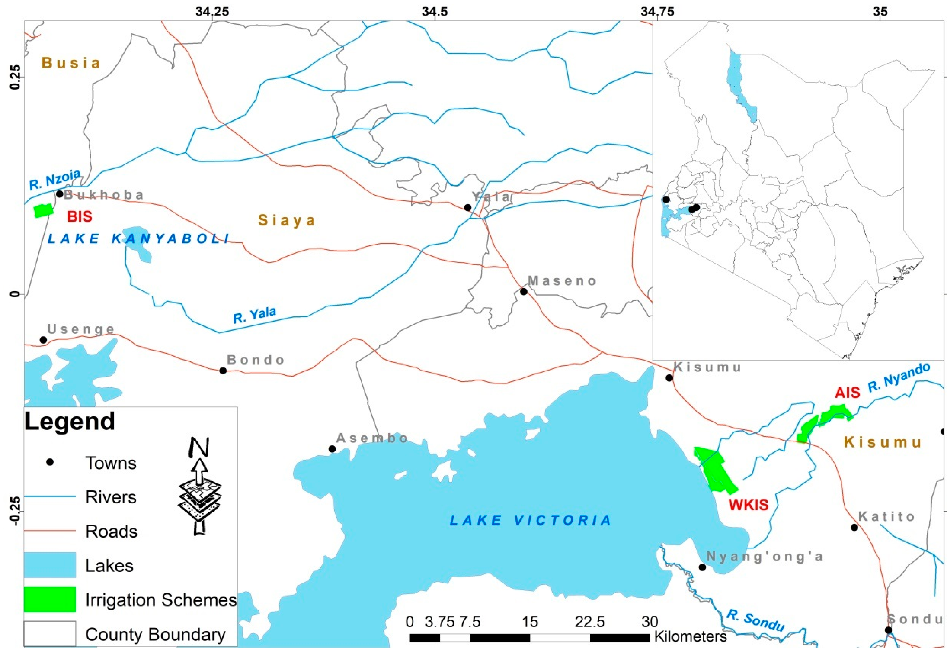
2.1. Description of Study Area

The study was carried out in the Ahero, West Kano and Bunyala irrigation schemes in western Kenya managed by National Irrigation Board NIB (Figure 1). Rice is the main crop grown in these schemes. In all the schemes, water is abstracted using electric-powered pumps, conveyed with open earth canals and applied using basin irrigation method. Drain water is pumped back to Lake Victoria in the West Kano irrigation scheme because the outlet is on lower ground than the lake. The schemes have no gauging stations. Western Kenya is hot and humid, with a bimodal rainfall pattern. The schemes are underlain by deep black cotton soils [22].

A detailed description of the main features of three irrigation schemes studied is presented in

Table 2. Main characteristics of irrigation schemes benchmarked in western Kenya.

Description	Irrigation Scheme
	Ahero	West Kano	Bunyala
Command area (ha)	900	980	728
Latitude	00°10′ South	Between 00°04′ South and 00°20′ South	00°06′ North
Longitude	34°58′ East	Between 34°48′ East and 35°02′ East	34°04′ East
Location	Kano plains, Kisumu county	Kano plains, Kisumu county	Kisumu/Siaya county
Land ownership	Government	Government	Government and private
Main crops	Rice, Soybeans, maize, Watermelon, sorghum	Rice, sorghum, maize	Rice, pulses and horticulture
Number of seasons	2 seasons 1st season-rice 2nd-other crop	2 seasons 1st season-rice 2nd-other crop	2 seasons 1st season-rice 2nd-other crop
Number of farmers	556	845	1934
Farm size (acres)	1–4	2–4	1–5
Water source	Surface water River Nyando	Surface water Lake Victoria	Surface water River Nzoia
Type of water distribution	On demand	On demand	On demand
Method of water abstraction	Pumping using electricity 2 pumps each 1100 L/s 2 pumps each 650 L/s	Pumping using electricity 3 pumps each 750 L/s	Pumping using electricity 4 pumps each 300 L/s
Water delivery infrastructure	Open earth canals	Open earth canals	Open earth canals
Type of water control equipment	None	None	None
Discharge measurement facilities	None	None	None
Irrigation system	Surface-Basin	Surface-Basin	Surface-Basin
Water availability	Sufficient-occasionally not sufficient	Abundant	Abundant
Type of surface drain	Open earth channel by gravity	Pumped through open earth channel. Using four 500 L/s outlet pumps.	Open earth channel
Type of revenue collection	Charge on irrigated area	Charge on irrigated area	Charge on irrigated area

.

2.2. Data Collection

Secondary time series data for five years (2012–2016) was obtained from records kept by management of the various irrigation schemes. The data collected was only for rice production. Rice is grown in the first season, while the other crops are grown in the second season. The production of the other crops has not been formalised, and their production is not documented. Data on total yield per season, local crop price per season, cropped area, total command area, revenue collected, expected revenue, cost of production, water supplied, pump speed, and pumping hours was collected from records kept by the irrigation scheme offices and field survey. Meteorological data was obtained from Ahero research station, West Kano weather station, the Kenya Meteorological Department (KMD) and the NASA POWER Centre. Key informant interviews, observation, and focus group discussion methods were used to collect data on farming practices, cropping pattern, status of the irrigation systems and maintenance of the system.

2.3. Data Analysis

Field data was first processed to obtain variables for calculating performance indicators. The variables were computed as follows:

(a)   Crop water requirement

Crop pattern, transplanting date and weather data was used in calculating rice crop water demand and crop irrigation water requirement using CROPWAT 8.0 software (developed by FAO, Rome, Italy). Computation of reference crop water demand (ET_o) is based on the Penman Monteith equation. The effective rainfall was computed using USDA-Soil Conservation Method, in-built in CROPWAT 8. Number of sunshine hours, temperature, humidity, rainfall data, wind speed, soil type, transplanting date and crop pattern were used as input for the model. The total annual volume of water consumed by all crops in the irrigation schemes was computed using Equation (8) [10].

$$VE{t}_c={\sum }_{crops}E{t}_c\times A$$

(8)

$VE{t}_c$ = Total volume of crop water demand (m³); Et_c = crop evapotranspiration from planting to harvesting (m³); A = cropped area.

Total annual volume crop irrigation demand was then calculated using Equation (9) [10].

$$VE{t}_{Net}=I{R}_{n}A$$

(9)

$VE{t}_{Net}$ = Total volume of water consumed by crops less effective rainfall (m³); $I{R}_n$ = net irrigation water requirement (m³); A = cropped area

(b)

Total annual volume of irrigation water supply (m³). This was obtained by summing the daily volume of water pumped for the rice growing season in each year. Daily volume of water pumped was obtained as the product of pump efficiency, pumping hours and the pump operating speed.

(c)

Total annual volume of water supply (m³). This was obtained by summing the total volume of water pumped for irrigation and total effective rainfall for the rice growing season in a year. The effective rainfall was computed using the USDA-Soil Conservation Method, in-built in CROPWAT 8. The effective rainfall in terms of depth was converted into volume by multiplying by the total annual cropped area.

(d)

Total annual cropped area (ha). This was calculated by summing up all the area under rice crop in each year.

(e)

Total command area of the system (ha). This is the net area serviced by the scheme less the right of way for canals, drains, roads and villages. It was obtained from the design office of each irrigation scheme.

The performance indicators used were obtained from the IPTRID benchmarking indicators presented in

Table 3. Proposed key performance indicators.

Domain	Performance Indicator	Data Required
Service delivery performance	Total annual volume of irrigation water delivery (m3/year)	Total daily measured water delivery to water users
	Annual irrigation water delivery per unit command area (m3/ha)	Total daily measured water inflow to the irrigation system
		Total command area serviced by the system
	Annual irrigation water delivery per unit irrigated area (m3/ha)	Total daily measured water inflow to the irrigation system
		Total annual irrigated crop area
	Main system water delivery efficiency	Total daily measured water delivery to water users
		Total daily measured water inflow to the irrigation system
	Annual relative water supply	Total daily measured water inflow to the irrigation system
		Total daily measured rainfall over irrigated area
		Total daily/periodic volume of crop water demand, including percolation losses for rice crops
	Annual relative irrigation supply	Total daily measured water inflow to the irrigation system
		Total daily/periodic volume of irrigation water demand (crop water demand excluding effective rainfall), including percolation losses for rice
	Water delivery capacity	Current main canal capacity
		Peak month irrigation water demand
	Security of entitlement supply	System water entitlement
		10 years minimum water availability flow pattern
Financial performance	Cost recovery ratio	Total revenues collected from water users
		Total management, operation and maintenance (MOM) cost
	Maintenance cost to revenue ratio	Total maintenance expenditure
		Total revenue collected from water users
	Total MOM cost per unit area (US$/ha)	Total management, operation and maintenance expenditure
		Total command area serviced by the system
	Total cost per person employed on water delivery (US$/person)	Total cost of MOM personnel
		Total number of MOM personnel employed
	Revenue collection performance	Total revenues collected from water users
		Total service revenue due
	Staffing numbers per unit area (persons/ha)	Total number of MOM personnel employed
		Total command area serviced by system
	Average revenue per cubic meter of irrigation water supplied (US$/m3)	Total revenues collected from water users
		Total daily measured water delivery to water users
Agricultural Productive efficiency	Total gross annual agricultural production (tones)	Total tonnage produced under each crop
	Total annual value of agricultural production (US$)	Total annual tonnage of each crop
	Output per unit serviced area (US$/ha)	Crop market price
		Total annual tonnage of each crop
		Crop market price
		Total command area serviced by system
	Output per unit irrigated area (US$/ha)	Total annual tonnage of each crop
		Crop market price
		Total annual irrigated crop area
	Output per unit irrigation supply (US$/m3)	Total annual tonnage of each crop
		Crop market price
		Total daily measured water inflow to the irrigation system
	Output per unit water consumed (US$/m3)	Total annual tonnage of each crop
		Crop market price
		Total volume of water consumed by the crops (ETc)
Environmental performance	Water quality: Salinity (mmhos/cm)	Total daily measured water inflow to the irrigation system
		Electrical conductivity of periodically collected drainage water samples
		Total daily measured drainage water outflow from the irrigation system
	Water quality: Biological (mg/litre)	Biological load of periodically collected irrigation water samples
		Total daily measured water inflow to the irrigation system
		Biological load of periodically collected drainage water samples
		Total daily measured drainage water outflow from the irrigation system
	Water quality: Chemical (mg/litre)	Chemical load of periodically collected irrigation water samples
		Total daily measured water inflow to the irrigation system
		Chemical load of periodically collected drainage water samples
		Total daily measured drainage water outflow from the irrigation system
	Average depth to water table (m)	Periodic depth measurement to water table
	Change in water table depth over time (m)	Periodic depth measurement to water table over 5 year period
	Salt balance (tones)	Periodic measurement of salt content of irrigation water
		Periodic measurement of salt content of drainage water

[10].

The methodology adopted entails: (i) selection of suitable indicators to describe performance of the irrigation schemes; (ii) combining the indicators into a single performance score using principal component analysis. Some of the proposed key performance indicators (Table 3) were not computed because of lack of data.

2.3.1. Performance Indicators

Fourteen performance indicators were computed as shown in

Table 4. Computation of performance indicators.

Performance Indicator	Definition/Calculation
Total annual volume irrigation supply	Total annual volume of irrigation water pumped or diverted
Annual relative water supply	$\frac{\mathrm{total} \mathrm{annual} \mathrm{volume} \mathrm{of} \mathrm{water} \mathrm{supply}}{\mathrm{total} \mathrm{annual} \mathrm{volume} \mathrm{of} \mathrm{crop} \mathrm{water} \mathrm{demand}}$
Annual relative irrigation supply	$\frac{\mathrm{total} \mathrm{annual} \mathrm{volume} \mathrm{of} \mathrm{irrigation} \mathrm{supply}}{\mathrm{total} \mathrm{annual} \mathrm{volume} \mathrm{of} \mathrm{crop} \mathrm{irrigatio} \mathrm{demand}}$
Annual irrigation supply per unit irrigated area (m3/ha)	$\frac{\mathrm{Total} \mathrm{annual} \mathrm{volume} \mathrm{of} \mathrm{irrigation} \mathrm{supply}}{\mathrm{Total} \mathrm{annual} \mathrm{irrigated} \mathrm{area}}$
Annual irrigation supply per unit command area (m3/ha)	$\frac{\mathrm{Total} \mathrm{annual} \mathrm{volume} \mathrm{of} \mathrm{irrigation} \mathrm{supply}}{\mathrm{Total} \mathrm{annual} \mathrm{command} \mathrm{area}}$
Total gross annual agricultural production (tones)	Total annual tonnage of each crop
Total annual valueof agricultural production (US$)	Total annual gross value of production (GVP) received by producers
Output per unit irrigated area (US$/ha)	$\frac{\mathrm{Total} \mathrm{annual} \mathrm{value} \mathrm{of} \mathrm{agricultural} \mathrm{production}}{\mathrm{Total} \mathrm{annual} \mathrm{irrigated} \mathrm{area}}$
Output per unit command area (US$/ha)	$\frac{\mathrm{Total} \mathrm{annual} \mathrm{value} \mathrm{of} \mathrm{agricultural} \mathrm{production}}{\mathrm{Total} \mathrm{command} \mathrm{area}}$
Output per unit water supply (US$/m3)	$\frac{\mathrm{Total} \mathrm{annual} \mathrm{value} \mathrm{of} \mathrm{agricultural} \mathrm{production}}{\mathrm{total} \mathrm{annual} \mathrm{volume} \mathrm{of} \mathrm{water} \mathrm{suply}}$
Output per unit irrigation supply (US$/m3)	$\frac{\mathrm{Total} \mathrm{annual} \mathrm{value} \mathrm{of} \mathrm{agricultural} \mathrm{production}}{\mathrm{total} \mathrm{annual} \mathrm{volume} \mathrm{of} \mathrm{irrigation} \mathrm{suply}}$
Output per unit crop water demand (US$/m3)	$\frac{\mathrm{Total} \mathrm{annual} \mathrm{value} \mathrm{of} \mathrm{agricultural} \mathrm{production}}{\mathrm{total} \mathrm{annual} \mathrm{volume} \mathrm{of} \mathrm{crop} \mathrm{water} \mathrm{demand}}$
Water fee collection performance (%)	$\frac{\mathrm{Gross} \mathrm{revenue} \mathrm{collected}}{\mathrm{Gross} \mathrm{revenue} \mathrm{invoiced}}\times 100$
Average revenue per unit irrigation supply (US$/m3)	$\frac{\mathrm{total} \mathrm{annual} \mathrm{revenue} \mathrm{collected} }{\mathrm{Total} \mathrm{annual} \mathrm{volume} \mathrm{of} \mathrm{irrigation} \mathrm{supply}}$

. The indicator values were compared among the three schemes in each year.

To allow for global comparison, the total value of agricultural production is converted into gross value of production using Equation (10).

$$GVP=\lfloor {\displaystyle \sum }crops{A}_i{Y}_i\rfloor \mathrm{MU} \mathrm{currency} \mathrm{exchange} \mathrm{rate}$$

(10)

GVP—gross value of production; A_i—area cropped with crop i; Y_i—the yield of crop i; P_i—local price of crop i; MU—currency exchange rate (US$ per unit local currency).

2.3.2. Calculation of Overall Irrigation Scheme Performance

The overall scheme performance was determined by computing a single performance score. The total volume of irrigation water supply, total annual agricultural production and total annual value of agricultural production indicators were excluded in the computation of overall performance score. These indicators are based on extensive scale rather than relative scale and their inclusion might distort the results. Indicators were first tested for statistical correlation using the Pearson correlation method. Ten indicators with low correlation were selected. The indicators were weighted using principal component analysis, then normalised using the reference to target method and finally aggregated into a single performance score using the linear aggregation method. Weighting of indicators was done using PCA.

Principal Component Analysis (PCA)

PCA was done using SPSS windows version16 software. Prior to PCA, the data was tested for suitability using Kaiser-Meyer-Olklin (KMO) and Bartlett Test of Sphericity (BTS). The extracted components were rotated using orthogonal varimax method to achieve significant components. The indicator weights were computed using rotated factor loadings and eigenvalues, as shown in Equation (11).

$$W_k={\displaystyle \sum }_{j=1}^{j=n}\frac{{({\mathrm{Factor} \mathrm{loading}}_{kj})}^2}{{\mathrm{eigenvalue}}_j}\times \frac{{\mathrm{eigenvalue}}_j}{{\sum }_{j=1}^{j=n}{\mathrm{eigenvalue}}_j}$$

(11)

${\mathrm{Factor} \mathrm{loading}}_{kj}$—factor loading of indicator k in the principal component j; ${\mathrm{eigenvalue}}_j$—eigenvalue for j^th principal component; j = 1, j = 2, …, j = n the extracted principal components with an eigenvalue above 1.

The indicators were normalised using reference to target using Equation (12).

$$I_{qs}^t=\frac{x_{qs}^t}{x_b}$$

(12)

$I_{qs}^t$ = normalised value of indicator q for scheme s at time t; $x_{qs}^t$ = indicator value for scheme s at time t; $x_b$= threshold value for indicator value.

The threshold values used for normalisation of indicators are shown in

Table 5. Indicative threshold values.

Performance Indicator	Threshold Values	Reference
Relative water supply	2	[23]
Relative irrigation supply	2	[23]
Annual irrigation water delivery per unit irrigated area	450–700 mm	[24]
Annual irrigation water delivery per unit command area	450–700 mm	[24]
Output per unit irrigated area	3.8 ton/ha	[25]
Output per unit command area	3.8 ton/ha	[25]
Output per unit irrigation supply	2 kg/m3	[26]
Output per unit water supply	2 kg/m3	[26]
Output per water consumed	2 kg/m3	[26]
Water fee collection performance	100%	[10]
Average revenue per unit irrigation supply	7.5 US dollar cents	[27]

.

A single performance score was finally computed using Equation (13).

$$C{I}_{st}={{\displaystyle \sum }}_{k=1}^{k=n}{W}_k{I}_{ks}$$

(13)

where; W_k = indicator weight; I_ks =normalised indicator k for scheme s; CI_st = performance score for irrigation scheme s at time t.

3. Results and Discussion

The results of comparative evaluation of performance using performance indicators are presented as follows.

3.1. Water Supply Performance

The indicators under this category give a measure of water supply relative to demand. Water abundance or scarcity of water can be deduced from these indicators [28]. The results of water supply indicators are presented in

Table 6. Water supply indicators.

Irrigation Scheme	Year	Command Area (ha)	Total Annual Irrigated Area (ha)	Total Annual Volume of Irrigation Water Supply (m3)	RWS	RIS	Annual Water Deliver per Unit Irrigated Area (m3/ha)	Annual Water Delivery per Unit Command Area (m3/ha)
Ahero	2012/2013	900	877	6,827,820	1.98	2.15	7785	7586
	2013/2014	900	846	4,938,460	1.14	0.86	5837	5487
	2014/2015	900	783	4,867,840	1.45	1.31	6217	5409
	2015/2016	900	824	4,362,330	1.28	0.86	5294	4847
	2016/2017	900	720	3,950,460	1.24	0.68	5487	4389
Average			810	4,989,382	1.42	1.17	6124	5544
West Kano	2012/2013	980	617	6,934,097	2.31	3.38	11,238	7076
	2013/2014	980	206	2,540,691	1.94	1.64	12,310	2593
	2014/2015	980	196	2,223,590	2.21	2.74	11,376	2269
	2015/2016	980	650	7,115,034	1.92	1.75	10,955	7260
	2016/2017	980	690	8,411,680	1.86	1.58	12,191	8583
Average			472	5,445,018	2.05	2.22	11,614	5556
Bunyala	2012/2013	728	701	4,406,847	1.98	1.94	6287	6050
	2013/2014	728	701	6,215,776	2.17	2.25	8868	8533
	2014/2015	728	701	5,401,296	2.06	2.26	7706	7415
	2015/2016	728	625	5,387,886	2.24	2.40	8622	7396
	2016/2017	728	666	8,077,590	2.44	2.46	12,130	11,089
Average			679	5,897,879	2.18	2.26	8723	8097

RWS—Relative Water Supply; RIS—Irrigation Water Supply.

. The command area and irrigated area used in computation of various performance indicators for each scheme is also presented in Table 6.

The available irrigable area (command area) in all the schemes has not been fully exploited. Some of the command area is not irrigated due to the inability of farmers to acquire farming inputs. Irrigated area in Ahero and Bunyala irrigation schemes is close to command area. The low irrigated area in West Kano in 2013 and 2014 can be attributed to lack of interest in irrigation by farmers following the collapse of the revolving fund committee. The annual volume of irrigation supply for the schemes ranges between 2.2 and 8.4 MCM. All the schemes divert water by pumping using electricity. The amount of water abstracted at any given time depends on cropped area. The irrigation schemes have a high fluctuation in the amount of water supplied due to frequent power outages experienced in the region. The amount of water abstracted is estimated using pumping hours recorded, pump speed and pumping efficiency. The amount of water delivered to irrigation blocks could not be computed.

The relative irrigation supply (RIS) values varied from 0.68 to 3.38 during the study period. RIS and RWS values should be above 1. This is because irrigation efficiency is always below 100% due to unavoidable conveyance and application losses. Values below 1 indicate water deficit [26,27]. The average RIS in the Ahero, west Kano and Bunyala irrigation schemes was 1.17, 2.22 and 2.26, respectively. A low RIS value of 0.4 was reported in Muda irrigation scheme, Malaysia [15]. The low RIS was associated with the use of real-time monitoring of water depth in rice farms, which enabled effective use of rainfall. The relative water supply (RWS) varied between 1.14 and 2.44 for all the schemes. RWS above 2 shows that the amount of water supplied is adequate [15]. High RIS and RWS values in the West Kano and Bunyala irrigation schemes show that there is adequate supply of water. The Ahero irrigation scheme suffers from inadequate supply of water, which is evident from the low RIS values, the majority of which are below 1. The Ahero irrigation scheme draws water from the river Nyando, which is occasionally affected by drought and siltation. The Ahero irrigation scheme was in drought, which lowered the amount of water available for irrigation in 2013. In 2016, one of the water pumps, with a discharge capacity (100 L/s), broke down. This contributed to a very low RIS of 0.68. The water shortage in all the irrigation schemes is due to frequent power outages.

The average RIS values obtained are comparable to the average RIS value of 2.31 recorded in the large public rice irrigation schemes in the Senegal Valley in Mauritania [18]. An average RWS of 0.77 was obtained in Karacabey surface irrigation system, Turkey [29]. This irrigation scheme was reported to have a water shortage. Elsewhere in Turkey, [30] obtained RWS values ranging between 0.37 and 1.97. In Malaysia, RWS varied between 0.4 and 4.3, while RIS ranged between 0.5 and 5.7. The high values in Malaysia are attributed to extensive rice farming using open channels. An average RIS value of 1.38 was obtained for sprinkler irrigation systems and 1.03 for drip irrigation systems in Spain [17]. Sprinkler and drip irrigation systems have a high irrigation efficiency compared to the surface irrigation method. That is why the RIS values are lower compared to the values obtained in the Ahero, Bunyala and West Kano irrigation schemes.

The quantity of water supplied per unit area varies with the availability of water, climate, soil type, cropping pattern, system conditions and system management [31]. The annual water delivery per unit command area (WDCA) varied between 2269 m³/ha (West Kano in 2014/2015) to 11,089 m³/ha (Bunyala in 2016/2017). The WDCA was 4389 m³/ha−7586 m³/ha in Ahero, 2269 m³/ha−8583 m³/ha in West Kano and 6050 m³/ha−11,089 m³/ha in the Bunyala irrigation scheme. WDCA was highest in Bunyala, and least in the Ahero irrigation scheme. The annual water delivery per unit irrigated area (WDIA) varied from 5294 m³/ha to 7785 m³/ha in Ahero; 11,238 m³/ha to 12,310 m³/ha in West Kano and 6285 m³/ha to 12,130 m³/ha in the Bunyala irrigation scheme. This is equivalent to supplied depth of water of 529.4 mm–778.5 mm in Ahero, 1123.8 mm–1231 mm in West Kano, and 628.5 mm to 12,130 mm in the Bunyala irrigation scheme. According to the FAO, the average crop water needed for paddy rice should be 450 mm–700 mm [32]. Considering low irrigation efficiencies associated with surface irrigation schemes—usually 30–40% [32]—the WDIA is adequate in the West Kano and Bunyala irrigation schemes. The Ahero irrigation scheme, on the other hand, supplies inadequate water, which is not enough to meet crop water needs. WDIA values are relatively lower compared to the 22,029.43 m³/ha, 16,026.37 m³/ha, 11,289.10 m³/ha, and 9795.96 m³/ha obtained in MARIIS, Divisoria, Lucban and Garab SWIPs, respectively, in the Cagayan river basin, Philippines [23]. In southern Italy, high WDIA values ranging between 6500–14,900 m³/ha were reported by the Water Users’ Association (WUA’s) of Calabria [33]. WDIA values of 5578 m³/ha were obtained in sprinkler irrigation systems and 1084 m³/ha in drip irrigation systems in Castilla-La Mancha, Spain [17]. These values are much lower than the values obtained in this study. Drip and sprinkler irrigation systems have high water application efficiencies of 75% and 90%, respectively [34]. Surface irrigation systems, on the other hand, have a low irrigation efficiency of 60%. Therefore, more water is supplied in surface irrigation systems compared to sprinkler and drip irrigation systems. In the Susurluk river basin in Turkey, WDCA values varying from 1465 m³/ha to 13,086 m³/ha and WDCA values ranging from 2169 m³/ha to 22,098 m³/ha were obtained [30]. A high amount of water is supplied to irrigation schemes in the Sursurluk basin because rainfall is limited during the irrigation period.

3.2. Financial Performance

The financial performance indicators measure the efficiency with which irrigation systems use resources to provide service to farmers [23]. The results are shown in

Table 7. Financial performance indicators.

		Gross Revenue Collected (US$)	Gross Revenue Invoiced (US$)	Revenue Collection Performance (%)	Average Revenue per Unit Irrigation Water Supply (US Dollar Cents /m3)
WKIS	2012/2013	24,979.50	55,510.00	45	0.36
	2013/2014	8910.72	18,564.00	48	0.35
	2014/2015	8966.41	17,581.20	51	0.40
	2015/2016	31,547.88	58,422.00	54	0.44
	2016/2017	35,375.34	62,062.00	57	0.42
	Average	21,955.97	42,427.84	51	0.39
AIS	2012/2013	67,208.00	53,766.40	80	0.79
	2013/2014	64,790.00	55,071.50	85	1.12
	2014/2015	59,985.00	49,187.70	82	1.01
	2015/2016	63,147.00	54,306.42	86	1.24
	2016/2017	55,180.00	49,662.00	90	1.26
	Average	62,062.00	52,398.80	85	1.08
BIS	2012/2013	69,280.00	63,737.60	92	1.45
	2013/2014	69,280.00	65,123.20	94	1.05
	2014/2015	69,280.00	64,430.40	93	1.19
	2015/2016	61,770.00	58,681.50	95	1.09
	2016/2017	65,820.00	63,811.20	97	0.79
	Average	67,086.00	63,156.78	94	1.11

Currency exchange rate—1 US$ = 100 Kenya shilling (KES).

.

Water fee collection performance (WFC) values obtained are 80–90% in the Ahero irrigation scheme, 45–57% in the West Kano irrigation scheme, and 92–97% in the Bunyala irrigation scheme. According to [18], water fee collection values below 70% are considered unsatisfactory. Bunyala has the highest average fee collection performance, at 94%, while West Kano has the lowest average value, at 51%. The ideal desirable value should be close to 100% [10]. De Alwis and Wijesekara [35] obtained an ideal WFC of 100% in the Beypazarı Başören irrigation system, Turkey. Similarly, a WFC of 103% was recorded in the Karacabey irrigation scheme in Turkey. Values of WFC equal to or above 100% show that water users are willing to pay for the cost of irrigation. WFC values above 100% are possible to obtain due to payment of accumulated arrears. Low WFC values point out an unwillingness of farmers to pay water fees, poor organisation of the Irrigation Water Users Association (IWUA), poor collection programs, and financial problems within the schemes. Bunyala is able to sustain a value above 90% because of the well-organised farmer groups that are mandated with the mobilisation of the water fee. Also, in Bunyala, the policy of water fee payment prior to ploughing is strictly followed.

The average revenue per unit cubic meter varied from 0.79 to 1.26 US cents in the Ahero irrigation scheme, 0.35 to 0.44 US cents in the West Kano irrigation scheme, and 0.79 to 1.45 US cents in the Bunyala irrigation scheme. These values are below the economic value of irrigation water of 7.54 US cents per cubic meter obtained by [27] in the Ahero irrigation scheme. Pricing of water is an economic aid to improving water allocation and sustainable water utilisation [30]. The water fee charged is US$31, US$36.40 and US$40 per acre in the Ahero, West Kano and Bunyala irrigation schemes, respectively. The pricing is based on area cropped per farming season and not the quantity of water consumed. There is no limit to the quantity of water that a farmer can use. This explains why the value of water per cubic meter is below 1 US$. This is a weakness and is unsuitable in terms of efficiency of water use and water conservation. Bunyala is the best performing irrigation scheme under the financial performance category.

3.3. Agricultural Productivity

Agricultural productivity gives the relationship between inputs and output. It gives an indication of efficiency of crop production in terms of land used, amount of water used and the income generated [36]. The indicators are presented in

Table 8. Agricultural productivity indicators.

Irrigation Scheme	Year	AGP (Tones)	GVP (US$)	OIA (US$/ha)	OCA (US$/ha)	OIS (US$/m3)	OWS (US$/m3)	OCWD (US$/m3)
West Kano	2012/2013	2679	857,120	950	1389	0.12	0.09	0.21
	2013/2014	1201	420,308	466	2036	0.17	0.13	0.26
	2014/2015	1136	374,959	416	1918	0.17	0.12	0.27
	2015/2016	3633	1,307,837	1450	2014	0.18	0.14	0.26
	2016/2017	4083	1,551,707	1720	2249	0.18	0.15	0.28
Average		2546	902,386	1000	1921	0.17	0.13	0.26
Ahero	2012/2013	4179	1,677,200	1864	1912	0.25	0.14	0.28
	2013/2014	4182	1,479,800	1644	1749	0.30	0.20	0.22
	2014/2015	4551	1,683,870	1871	2151	0.35	0.20	0.29
	2015/2016	4465	1,741,370	1935	2113	0.40	0.21	0.27
	2016/2017	4058	1,663,780	1849	2311	0.42	0.22	0.28
Average		4287	1,649,204	1832	2047	0.34	0.20	0.27
Bunyala	2012/2013	3803	1,248,221	1714	1781	0.28	0.15	0.29
	2013/2014	2146	714,678	981	1020	0.11	0.07	0.16
	2014/2015	3380	1,132,300	1554	1615	0.21	0.13	0.26
	2015/2016	3850	1,321,617	1814	2115	0.25	0.15	0.34
	2016/2017	3633	1,214,772	1668	1824	0.15	0.11	0.28
Average		3362	1,126,318	1546	1671	0.20	0.12	0.27

AGP—annual gross agricultural production; GVP—gross value of agricultural production; OIA—output per unit irrigated area; OCA—output per unit command area; OIS—output per unit irrigation supply; OCWD—output per unit crop water demand; Currency exchange rate—1 US$ = 100 Kenya shilling (KES).

.

The output per unit irrigation supply (OIS) ranges between 0.11 US$/m³ and 0.42 US$/m³ in all the schemes. The average, OIS is 0.34 US$/m³ in Ahero, 0.17 US$/m³ in West Kano, and 0.20 US$/m³ in the Bunyala irrigation scheme. Ahero irrigation scheme utilises water more efficiently compared to the others. The output per unit water supply (OWS) puts into consideration the contribution of effective rainfall. The values vary between 0.07 and 0.22 US$/m³. The highest OCWD value (0.34 US$/m³) was obtained in the Bunyala irrigation scheme in 2015/2016, while the lowest value (0.16 US$/m³) was recorded in Bunyala in 2013/2014. The Ahero and Bunyala irrigation schemes have the highest average OCWD of 0.27 US$/m³, while West Kano irrigation scheme has the lowest average value of 0.26 US$/m³. The Ahero irrigation scheme is leading in terms of water productivity while West Kano is the poorest. According to [15], if OCWD is greater than OIS, some of the irrigation water supplied is unproductive. In both West Kano and Bunyala, OIS is greater than OCWD. This shows inefficient use of water. The Ahero irrigation scheme is the most efficient water user, with all OIS values less than OCWD except in 2012/2013. The difference in water productivity is brought about by differences in yield and crop market price. In similar studies in Malaysia, [37] reported OWS values ranging between 0.01 US$/m³ and 0.2 US$/m³ and OCWD values varying from 0.01 US$/m³ to 0.4 US$/m³ for paddy rice. Compared to this, the Ahero, West Kano and Bunyala irrigation schemes registered higher rice water productivity. The difference is attributed to the yield and market price. Mchele [38] obtained OIS values of 0.95 US$/m³ in Shina-Hamusit and 0.62 US$/m³ in the Selamko irrigation scheme, and OCWD values of 1.46 US$/m³ in Shina-Hamusit and 1.15 US$/m³ in the Selamko irrigation scheme, Ethiopia. These irrigation schemes do not grow rice. This shows that rice is a competitive crop in terms of returns per water used. In Turkey, OCWD values varying between 0.191 US$/m³ and 1.262 US$/m³ were obtained [30]. The highest values of rice water productivity of 1.77 kg/m³, 1.75 kg/m³ and 1.51 kg/m³ have been reported in the USA, Sri Lanka and Spain, respectively [26].

Land productivity indicators give a reflection of crop intensity [39]. The output per unit command area (OCA) varies between 1020 US$/ha (Bunyala in 2013/2014) and 2311 US$/ha (Ahero in 2016/2017). The average OCA computed was 2047 US$/ha in Ahero; 1921 US$/ha in West Kano and 1671 US$/ha in the Bunyala irrigation scheme. A high value is an indication of intensive irrigation. The sudden fall in output per command area in West Kano between 2012 and 2014 can be attributed to the collapse of the Revolving Fund Committee. The committee was mandated with the responsibility for production and marketing in the West Kano irrigation scheme. Consequently, there was a decline in production activities during that period associated with governance issues. From 2015 each block in the scheme established a production management structure which induced competition amongst the blocks in terms of production activities. An increase in production was therefore realised in 2015/2016. The Bunyala irrigation scheme experienced hail in 2013 which shattered mature rice crops in one of the phases (Muluwa phase 1). This contributed to a low harvest, as depicted by the sudden decline in the output per unit area in the scheme. The output per unit irrigated area (OIA) for all the schemes varied from 981 US$/ha to 1841 US$/ha. The OIA values computed are comparable to the OIA values of 1300 US$/ha and 1310 US$/ha obtained during the rainy season and dry season in rice farming in Thailand [40]. OIA values ranging from 100 US$/ha to 800 US$/ha were reported in Malaysia [37].

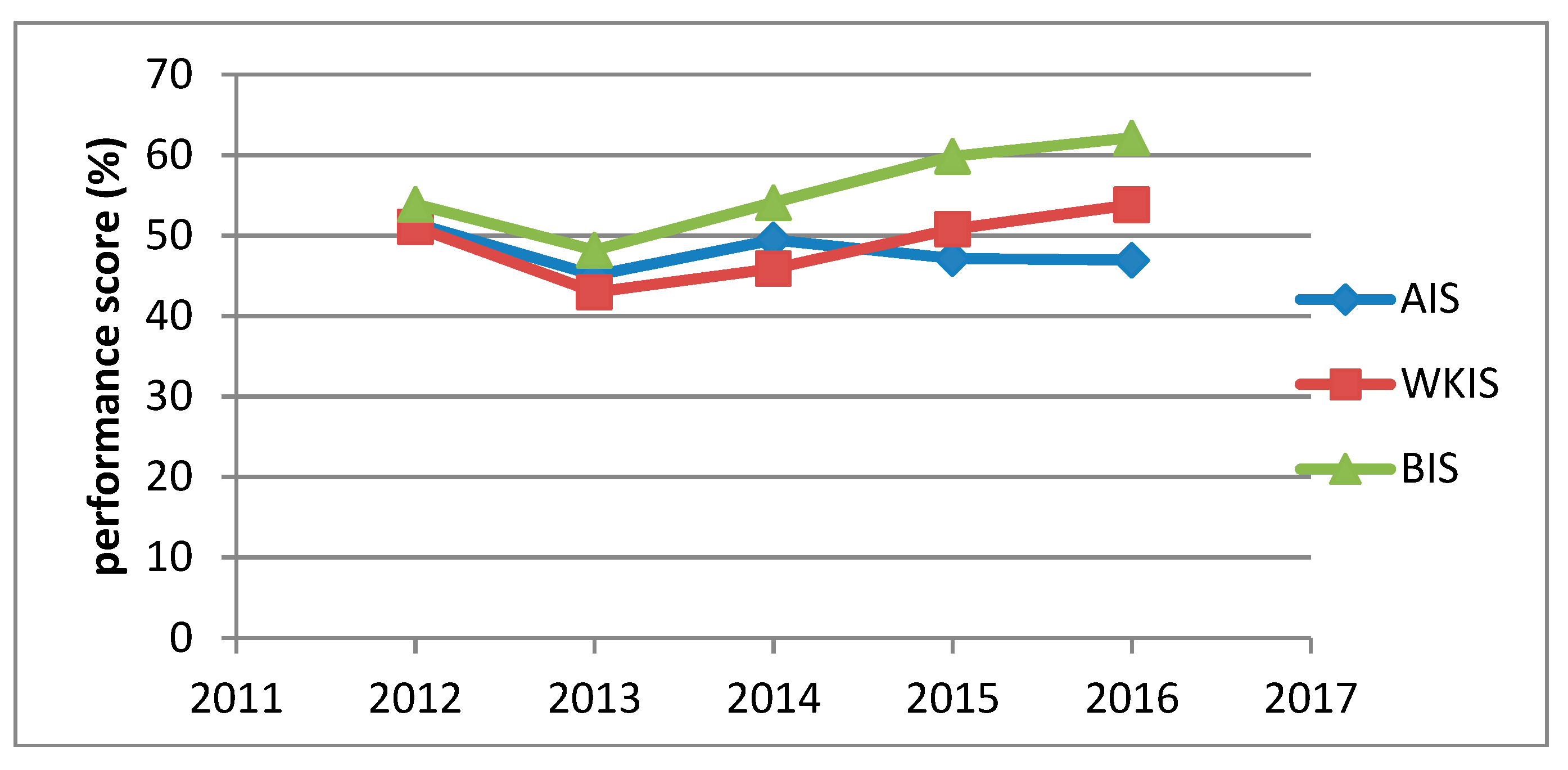
3.4. Estimation of Overall Scheme Performance

Correlation analysis of the 11 selected indicators is presented in

Table 9. Pearson correlation matrix (n).

Variables	RWS	RIS	WDIA	WDCA	WFC	RIWS	OIA	OCA	OIS	OCWD	OWS
RWS	1	0.950	0.711	0.458	−0.168	−0.425	−0.185	−0.305	−0.801	0.278	−0.855
RIS	0.950	1	0.648	0.455	−0.259	−0.457	−0.273	−0.292	−0.778	0.189	−0.845
ISIA	0.711	0.648	1	0.283	−0.645	−0.873	0.092	−0.570	−0.870	0.060	−0.701
ISCA	0.458	0.455	0.283	1	0.284	−0.029	−0.312	0.475	−0.432	−0.047	−0.471
WFC	−0.168	−0.259	−0.645	0.284	1	0.889	−0.180	0.696	0.469	0.125	0.278
ARIS	−0.425	−0.457	−0.873	−0.029	0.889	1	−0.125	0.662	0.723	0.109	0.514
OIA	−0.185	−0.273	0.092	−0.312	−0.180	−0.125	1	0.156	0.375	0.741	0.553
OCA	−0.305	−0.292	−0.570	0.475	0.696	0.662	0.156	1	0.566	0.301	0.480
OIS	−0.801	−0.778	−0.870	−0.432	0.469	0.723	0.375	0.566	1	0.217	0.936
OWC	0.278	0.189	0.060	−0.047	0.125	0.109	0.741	0.301	0.217	1	0.245
OWS	−0.855	−0.845	−0.701	−0.471	0.278	0.514	0.553	0.480	0.936	0.245	1

RWS—relative water supply; RIS—relative irrigation supply; WDIA—Water delivery per unit irrigated area; WDCA—water delivery per unit command area; WFC—water fee collection; RIWS—annual revenue per unit irrigation water supply; OIA—output per unit irrigated area; OCA—output per unit command area; OIS—output per unit irrigation supply; OCWD—output per unit crop water demand; OWS—output per unit water supply.

. RWS and RIS are strongly positively correlated (r = 0.950). This means that the indicators measure similar elements. To avoid double counting, only one of them can be used in the computation of the composite indicator/performance score. RIS focuses on irrigation water supply alone and is therefore used for computation of the performance score.

Principal Component Analysis

The extracted principal factors, Kaiser-Meyer-Olkin (KMO) measure of sampling adequacy and Bartlett’s sphericity test (BTS) results are presented in

Table 10. Kaiser-Meyer-Olkin (KMO) and Bartlett’s test.

KMO and Bartlett’s Test
Kaiser-Meyer-Olkin Measure of Sampling Adequacy.		0.510
Bartlett’s Test of Sphericity	Approx. Chi-Square	211.443
	df	45
	Sig.	0.000

.

According to [41], if the KMO value is greater than 0.5 and the BTS less than 0.05, the data is suitable for PCA. In this study, the KMO co-efficient of 0.510 is adequate and the Bartlett’s test is significant at 99% (p < 0.0001). The principal components extracted with their factor loadings are presented in

Table 11. The extracted principal components.

Rotated Component Matrix (Factor Loading)				Indicator Weights
	Principal Component
	1	2	3
% of variance	34.959	34.918	19.930
Relative irrigation supply (RIS)	−0.222	−0.876	0.044	0.091
Water delivery per unit irrigated area (WDIA)	−0.673	−0.669	0.169	0.104
Water delivery per unit command area (WDCA)	0.447	−0.794	−0.047	0.093
Water fee collection performance (WFC)	0.924	0.064	−0.068	0.096
Average revenue per unit irrigation water supply (RIWS)	0.862	0.387	−0.086	0.100
Output per unit irrigated area (OIA)	−0.161	0.317	0.912	0.107
Output per unit command area (OCA)	0.891	0.040	0.289	0.098
Output per unit irrigation supply (OIS)	0.505	0.815	0.229	0.108
Output per crop water demand (OCWD)	0.149	−0.081	0.925	0.098
output per unit water supply (OWS)	0.318	0.848	0.353	0.105
Extraction Method: Principal Component Analysis. Rotation Method: Varimax with Kaiser Normalisation.

. The indicator weights are also presented in this Table 11.

The first principal component (PC1) determines 34.9595% of the total variance in performance. The first principal component is mainly linked to indicators with absolute factor loading greater than 0.673 (WDIA, WFC, RIWS, OCA). The second principal component (PC2) accounts for 34.918% of the variance in performance. It is influenced by RIS, WDCA, OIS and OWS indicators (absolute loadings > 0.794). The third principal component (PC3) factor loading accounts for 19.93% and is linked with OIA and OCWD indicators.

The results of weighted indicators are presented in

Table 12. Weighted performance score for each category.

Year	IS	RIS	WSIA	WSCA	WFC	ARIWS	OIA	OCA	OIS	OCWD	OWS	PS
2012/2013	AIS	0.10	0.07	0.06	0.08	0.01	0.06	0.05	0.03	0.03	0.02	0.52
	WKIS	0.14	0.10	0.06	0.04	0.00	0.05	0.03	0.02	0.03	0.02	0.51
	BIS	0.09	0.06	0.05	0.09	0.02	0.07	0.06	0.05	0.04	0.02	0.54
2013/2014	AIS	0.04	0.05	0.05	0.08	0.01	0.06	0.05	0.05	0.03	0.03	0.45
	WKIS	0.07	0.11	0.02	0.05	0.00	0.07	0.01	0.03	0.04	0.02	0.43
	BIS	0.10	0.08	0.07	0.09	0.01	0.04	0.03	0.02	0.02	0.01	0.48
2014/2015	AIS	0.06	0.06	0.04	0.08	0.01	0.07	0.06	0.05	0.04	0.03	0.49
	WKIS	0.11	0.10	0.02	0.05	0.01	0.07	0.01	0.03	0.04	0.02	0.46
	BIS	0.10	0.07	0.06	0.09	0.02	0.06	0.05	0.03	0.04	0.02	0.54
2015/2016	AIS	0.04	0.05	0.04	0.08	0.02	0.07	0.06	0.06	0.03	0.03	0.47
	WKIS	0.09	0.10	0.07	0.05	0.01	0.07	0.04	0.03	0.04	0.02	0.51
	BIS	0.11	0.08	0.06	0.09	0.01	0.07	0.06	0.04	0.05	0.02	0.60
2016/2017	AIS	0.04	0.05	0.04	0.09	0.02	0.07	0.05	0.06	0.03	0.03	0.47
	WKIS	0.08	0.11	0.08	0.05	0.01	0.07	0.05	0.03	0.04	0.02	0.54
	BIS	0.11	0.11	0.09	0.09	0.01	0.07	0.06	0.02	0.04	0.02	0.62

IS—Irrigation scheme; AIS—Ahero irrigation scheme; WKIS—WKano irrigation scheme; BIS—Bunyala irrigation scheme; RIS—relative irrigation supply; WSIA—irrigation supply per unit irrigated area; WSCA—irrigation supply per unit command area; WFC—water fee collection; ARIWS—annual revenue per unit irrigation supply; OIA—output per unit irrigated area; OCA—output per unit command area; OIS—output per unit irrigation supply; OCWD—output per unit water consumed; OWS—output per unit water supply.

. The performance score for each scheme in each year was obtained by summing up the weighted indicator values.

Comparison of the trend in irrigation scheme performance of each scheme is presented in Figure 2.

The overall performance score obtained was 45–52% in Ahero, 43–54% in West Kano and 48–62% in the Bunyala irrigation scheme. The average performance was 48%, 49% and 56% in the Ahero, West Kano and Bunyala irrigation schemes, respectively. The performance in all of the schemes was moderate. The performance in the West Kano and Bunyala irrigation schemes increased with time. The performance in the Ahero irrigation scheme was seen to be decreasing with time. The West Kano irrigation scheme experienced a fall in performance in 2014 due to the collapse of the Revolving Fund Committee which was mandated with the responsibility of production and marketing. The establishment of the production management structure, which created competition among the blocks in terms of production, increased performance from 2015. The sudden decline in performance in Bunyala in 2013 was due to hail stones that shattered mature rice crops in one of the phases (Muluwa phase 1). The reduction in the amount of water available due to drought led to a decrease in performance in the Ahero irrigation scheme in 2013. In 2013, there was strong sensitisation in the System of Rice Intensification (SRI) technology in Ahero. SRI involves changes in plants, water soil and nutrients management aimed at increasing productivity of rice under irrigation. Most farmers in the Ahero irrigation scheme adopted SRI, which led to an increase in performance from 45% in 2013 to 49% in 2014. A high performance of 83% [12] was obtained in the Samrat Ashok Sagar major irrigation project in India using a balanced score card method based on the Delphi technique. Agricultural productivity in India is highly enhanced by the government through artificial fixing of the minimum price of crops. The prices are therefore reasonably high, leading to the high economic value of crops. This is not the case in Kenya, where the price of rice produce is governed by market forces. In times of surplus, rice fetches low prices, reducing its economic value. This contributes greatly to low agricultural productivity performance, leading to low overall performance of irrigation schemes. Zema and Nicotra [42] used PCA to identify areas of weakness in seven Water Users’ Association (WUA’s) in Calabra, Southern Italy. The Ionio Catanzarese (ICZ) WUA was ranked as the best performing with a quality index of 4470, while the Basso Ionio Reggino (BIRC) was found to be the least performing with a quality index of −1410. BIRC was found to have a weakness in both system operation performance and financial management. Lowering water prices was found to be the solution to improving performance of BRIC WUA’s in Calabra, Southern Italy [42].

4. Conclusions

The combination of benchmarking and Principal Component Analysis forms a powerful tool for evaluating the efficiency of irrigation schemes. The quantitative evaluation of performance of three rice irrigation schemes in western Kenya using a set of benchmarking indicators revealed the areas that needed improvement. Analysis of water supply indicators shows that, the water supplied by the irrigation schemes is sufficient to meet crop water demands. The irrigation schemes have low water use efficiency. In terms of financial performance, the irrigation schemes are not financially self-sufficient. The water fee charged was not sufficient to pay for the cost of irrigation. Land and water productivity in western Kenyan rice irrigation schemes was found to be generally good. Computation of a single performance score using performance indicators and principal component analysis enabled ranking of the irrigation schemes. The Bunyala irrigation scheme was found to be the best performing scheme, whereas the Ahero irrigation scheme was the least performing in the region. The overall performance of public rice irrigation schemes in western Kenya is average. Operation and management measures should be put in place to improve performance. The schemes need to adopt a systematic routine data collection and management to aid in the monitoring and evaluation of performance. Stakeholders and scheme managers can use this information to reformulate policies and strategies to enhance performance of public rice irrigation schemes in Kenya.

References

1. Government of Kenya. National Water Master Plan 2030 in the Republic of Kenya Final Report Volume -v Sectoral Report (2/3); Government of Kenya: Nairobi, Kenya, 2013.
2. Ngenoh, E.; Kirui, L.K.; Mutai, B.K.; Maina, M.C.; Koech, W.; Victoria, L. Economic Determinants of the Performance of Public Irrigation Schemes in Kenya. J. Dev. Agric. Econ. 2015, 7, 344–352. [Google Scholar] [CrossRef]
3. Gitonga, K. Grain and Feed Annual 2017 Kenya Corn, Wheat and Rice Report; USDA Foreign Agricultural Service: Washington, DC, USA, 2017.
4. Ministry of Water and Irrigation. Irrigation Sub-Sector MTP111 Zero Draft (2); Ministry of Water and Irrigation: Nairobi, Kenya, 2017.
5. Evans, A.A.; Florence, N.O.; Eucabeth, B.O.M. Production and Marketing of Rice in Kenya: Challenges and Opportunities. J. Dev. Agric. Econ. 2018, 10, 64–70. [Google Scholar] [CrossRef]
6. Kenya National Bureau of Statistics (KNBS). Economic Survey of Kenya; KNBS: Nairobi, Kenya, 2016.
7. Kenya National Bureau of Statistics (KNBS). Kenya Population Census Report; KNBS: Nairobi, Kenya, 2010.
8. Krhoda, G.O. Kenya National Water Development Report; UN-Water: Geneva, Switzerland, 2006; pp. 1–244. [Google Scholar]
9. Ngigi, S.N. Review of Irrigation Development in Kenya. In The Changing Face of Irrigation in Kenya: Opportunities for Anticipating Change in Eastern and Southern Africa; Blank, H.G., Mutero, C.M., Murray-Rust, H., Eds.; International Water Management Institute (IWMI): Colombo, Sri Lanka, 2002; Volume XIV, pp. 35–54. [Google Scholar]
10. Malano, H.; Burton, M.; Makin, I. Guidelines for Benchmarking Performance in the Irrigation and Drainage Sector, 1st ed.; International Programme for Technology and Research in Irrigation and Drainage (IPTRID) Knowledge Synthesis Report No. 5; FAO: Rome, Italy, 2001; Volume 53. [Google Scholar]
11. Malano, H.; Hungspreug, S.; Plantey, J.; Bos, M.G.; Vlotman, W.F.; Molden, D.; Burton, M. Benchmarking of Irrigation and Drainage Projects; International Commission on Irrigation and Drainage (ICID): New Delhi, India, 2004. [Google Scholar]
12. Phadnis, S.S.; Kulshrestha, M. Evaluation for Measuring Irrigation Service Performance Using a Scorecard Framework. Irrig. Drain. 2013, 62, 181–192. [Google Scholar] [CrossRef]
13. Renault, D.; Facon, T.; Wahaj, R. Modernizing Irrigation Management: The MASSCOTE Approach-Mapping System and Services for Canal Operation Techniques; Food and Agriculture Organization: Rome, Italy, 2007; Volume 63. [Google Scholar]
14. Burt, C.M.; Styles, S.W. Rapid Appraisal Process (RAP) and Benchmarking. Bioresour. Agric. Eng. 2001, 32–80. [Google Scholar]
15. Molden, D.; Sakthivadivel, R.; Perry, C.J.; De Fraiture, C.; Kloezen, W.H. Indicators for Comparing Performance of Irrigated Agricultural Systems; IWMI: Colombo, Sri Lanka, 1998; ISBN 9290903562. [Google Scholar]
16. Rodríguez Díaz, J.A.; Camacho-Poyato, E.; López-Luque, R.; Perez-Urrestarazu, L. Benchmarking and Multivariate Data Analysis Techniques for Improving the Efficiency of Irrigation Districts: An Application in Spain. Agric. Syst. 2008, 96, 250–259. [Google Scholar] [CrossRef]
17. Córcoles, J.I.; de Juan, J.A.; Ortega, J.F.; Tarjuelo, J.M.; Moreno, M.A. Evaluation of Irrigation Systems by Using Benchmarking Techniques. J. Irrig. Drain. Eng. 2012, 138, 225–234. [Google Scholar] [CrossRef]
18. Borgia, C.; García-Bolaños, M.; Li, T.; Gómez-Macpherson, H.; Comas, J.; Connor, D.; Mateos, L. Benchmarking for Performance Assessment of Small and Large Irrigation Schemes along the Senegal Valley in Mauritania. Agric. Water Manag. 2013, 121, 19–26. [Google Scholar] [CrossRef]
19. Jamilah, M.; Zakaria, A.; Md. Shakaff, A.Y.; Idayu, N.; Hamid, H.; Subari, N.; Mohamad, J. Principal Component Analysis—A Realization of Classification Success in Multi Sensor Data Fusion. In Principal Component Analysis—Engineering Applications; InTech: Philadelphia, PA, USA, 2012; pp. 1–25. [Google Scholar] [CrossRef]
20. Paul, L.C.; Suman, A.A.; Sultan, N. Methodological Analysis of Principal Component Analysis (PCA) Method. Int. J. Comput. Eng. Manag. 2013, 16, 32–38. [Google Scholar]
21. OECD. Handbook on Constructing Composite Indicators: Methodology and User Guide; OECD Publishing: Paris, France, 2008. [Google Scholar]
22. Kipkorir, E.C. Rice productivity, Water and Sanitation Baseline Survey Report Western Kenya Rice Irrigation Schemes. Available online: https://www.researchgate.net/publication/322686337_Rice_productivity_Water_and_Sanitation_Baseline_Survey_Report_Western_Kenya_Rice_Irrigation_Schemes (accessed on 11 October 2018).
23. Balderama, O.F.; Bareng, J.L.R.; Alejo, L.A. Benchmarking for Performance Assessment of Irrigation Schemes: The Case of National Irrigation Systems and Small Water Impounding Projects in Cagayan River Basin. In Proceedings of the International Conference of Agricultural Engineering, Zurich, Switzerland, 6–10 July 2014. [Google Scholar]
24. Brouwer, C.; Heibloem, M. Irrigation Water Management: Irrigation Water Needs. Train. Man. 1986, 3, 225–240. [Google Scholar]
25. Bastiaanssen, W.; Perry, C. Agricultural Water Use and Water Productivity in the Large Scale Irrigation (LSI) Schemes of the Nile Basin; Nile Information System: Entebbe, Uganda, 2009. [Google Scholar]
26. Bastiaanssen, W.G.M.; Steduto, P. The Water Productivity Score (WPS) at Global and Regional Level: Methodology and First Results from Remote Sensing Measurements of Wheat, Rice and Maize. Sci. Total Environ. 2017, 575, 595–611. [Google Scholar] [CrossRef] [PubMed]
27. Omondi, S.O. Economic Valuatio of Irrigation Water in Ahero Irrigation Scheme; University of Nairobi: Nairobi, Kenya, 2014. [Google Scholar]
28. Bos, M.G.; Burton, M.A.; Molden, D.J. Irrigation and Drainage Performance Assessment Practical Guidelines; CABI Publishing: Wallingford, UK, 2005; ISBN 0851999670. [Google Scholar]
29. Kuscu, H.; Bölüktepe, F.E.; Demir, A.O. Evaluation Performance of Irrigation Water Management: A Case Study of Karacabey Irrigation Scheme in Turkey. Int. J. Agric. Sci. 2015, 5, 824–831. [Google Scholar]
30. Kuşçu, H. Benchmarking Performance Assessment of Irrigation Water Management in a River Basin: Case Study of the Susurluk River Basin, Turkey. Afr. J. Bus. Manag. 2012, 6, 2848–2859. [Google Scholar] [CrossRef]
31. Government of Maharashtra. Report on Benchmarking of Irrigation Projects in Maharashtra; Government of Maharashtra: Mumbai, India, 2005.
32. Brouwer, C.; Prins, K.; Heibloem, M. Irrigation Water Management: Irrigation Scheduling. Train. Man. 1989, 4, 66. [Google Scholar]
33. Zema, D.A.; Nicotra, A.; Zimbone, S.M. Diagnosis and Improvement of the Collective Irrigation and Drainage Services in Water Users’ Associations of Calabria (Southern Italy). Irrig. Drain. 2018. [Google Scholar] [CrossRef]
34. Brouwer, C.; Prins, K.; Kay, M.; Heibloem, M. Irrigation Water Management: Irrigation Methods. Train. Man. 1998, 5, 140. [Google Scholar]
35. Cin, S.; Çakmak, B. Assessment of Irrigation Performance in Başören Irrigation Cooperative Area of Beypazarı, Ankara. J. Agric. Fac. Gaziosmanpasa Univ. 2017, 34, 10–19. [Google Scholar] [CrossRef]
36. De Alwis, S.M.D.L.K.; Wijesekara, N.T.S. Comparison of Performance Assessment Indicators for Evaluation of Irrigation Scheme Performances in Sri Lanka. Engineer 2011, 44, 39–50. [Google Scholar] [CrossRef]
37. Ghazalli, M.A. Benchmarking of Irrigation Projects in Malaysia: Initial Implementation Stages and Preliminary Results. Irrig. Drain. 2004, 53, 195–212. [Google Scholar] [CrossRef]
38. Shenkut, A. Performance Assessment Irrigation Schemes According to Comparative Indicators: A Case Study of Shina-Hamusit and Selamko, Ethiopia. Int. J. Sci. Res. Publ. 2015, 5, 451–460. [Google Scholar]
39. Mchele, A.R. Summary for Policymakers. In Climate Change 2013—The Physical Science Basis; Intergovernmental Panel on Climate Change, Ed.; Cambridge University Press: Cambridge, UK, 2011; Volume 53, pp. 1–30. [Google Scholar]
40. Bumbudsanpharoke, W.; Prajamwong, S. Performance Assessment for Irrigation Water Management: Case Study of the Great Chao Phraya Irrigation Scheme. Irrig. Drain. 2015, 64, 205–214. [Google Scholar] [CrossRef]
41. Kalantari, K.H. Processing and Analysis of Economic Data in Social Research. Publ. Consult. Eng. Landsc. Des. Tehran 2008, 3, 110–122. [Google Scholar]
42. Zema, D.A.; Nicotra, A.; Tamburino, V. Performance Assessment of Collective Irrigation in Water Users’ Associations of Calabria (Southern Italy). Irrig. Drain. 2015, 64, 314–325. [Google Scholar] [CrossRef]
Figure 1. Study Area.
Agriculture 08 00162 g001
Figure 2. Comparison of performance score.
Agriculture 08 00162 g002