Optimal and Robustly Optimal Consumption of Stretch Film Used for Wrapping Cylindrical Baled Silage

Abstract

A conventional method for wrapping round bales of agricultural materials by wrappers with a rotating table or with rotating arms is considered. In contemporary agriculture, the demand for minimal consumption of the film used to wrap bales is very high, in order to apply this method with lower cost and less damage to the environment. A combined model-based problem of such a design, focusing on the width of stretch film and the overlap between adjacent film strips that minimizes film consumption, was mathematically formulated and solved. It was proven that the complete set of optimal film widths is defined by a simple algebraic equation described in terms of film, bale, and wrapping parameters. The optimal overlap ratios were found to be irreducible fractions in which the dividend is the divisor minus one; however, only the first three factions, $\frac{1}{2},\frac{2}{3},\mathrm{and}\frac{3}{4}$, are practically significant. Next, the robustness to disturbances in the functioning of an actual bale wrapper, which leads to overlap ratio uncertainty, is examined. It was shown that, unfortunately, the optimal film widths applied together with the optimal overlaps do not provide any robustness to overlap variations. To overcome this inconvenience, the problems of a choice of the best commercially available film width guaranteeing minimal film consumption or maximal tolerance on the overlap uncertainty were formulated and solved. A new algorithm for a robust design of wrapping parameters was developed, motivated, and numerically verified to achieve a trade-off between satisfactory robustness and low film usage. For the resulting wrapping parameters, near-optimal film usage was achieved; the relative errors of the minimal film consumption approximation did not exceed 4%. It was proven that for the overlap, slightly more than 50%, i.e., 51% or 52%, provides both optimality and robustness of the overlap over disturbances, which are ensured regardless of the number of film layers. Moreover, it was found that for these overlaps and for the commercially available film widths selected according to the algorithm, the film consumption was more than twice as small than the film usage for exactly 50% overlap, if the actual overlap was smaller than pre-assumed. Similarly, an overlap of slightly more than the commonly used 67% will result in about 30% to 40% reduction in film usage in the presence of unfavorable disturbances, depending on the number of film layers and wrapping parameters.

1. Introduction

Baling technology has been widely used in storing agricultural materials, both at large feed factories and small-scale farms, due to the mechanization of the production chain, low labor requirements, ease of the manipulation and transport of bales, and low requirements for bale storage [1,2,3]. A persistently exciting bale wrapping application is that of silage conservation. Bales are wrapped in plastic film to ensure proper fermentation in anaerobic conditions without the need to build dedicated structures [4,5]. Comprehensive reviews of the literature, substantial and multifaceted, concerning physical and biochemical characteristics of baled silages with fermentation and nutritive quality [6,7,8] provide detailed information about the progress in bale silage conservation techniques [7,9,10], recent experimental studies [6,7], and future perspectives [7,8,10]. Although other silage conservation technologies are poised to replace baled silage for the primary purpose of providing good silage at low cost, it is likely to remain popular in the foreseeable future [7,11].

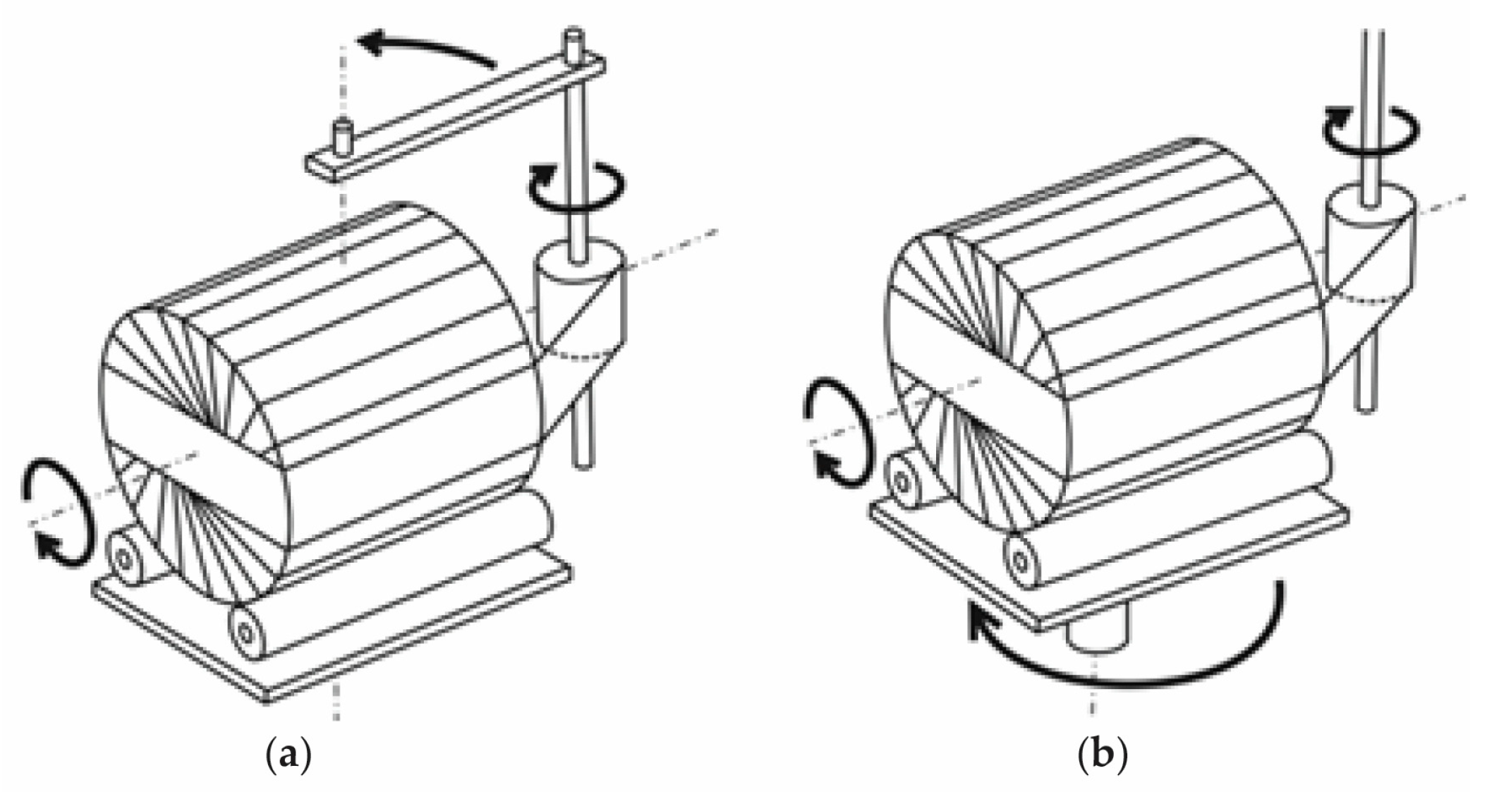
Today’s silage conservation in many regions of Europe [9,12], America [9], and China [1,11], especially for small and mid-sized producers, prefers round (i.e., cylindrical) bales wrapped individually. Since its origin in the 1980s, the conventional wrapping technique, according to which film strips are wrapped along the longitudinal axis of a bale, from the base to the top or vice versa, resulting in successive film layers, has been at the heart of the modern bale silage technique. Two main types of such round-bale wrappers are available [13,14]. In the first type, the film is applied by a pre-stretching unit mounted on an arm rotating around the bale (Figure 1a); see also [15]. The second type uses a rotating table on which the bale is rotated around its longitudinal axis, as seen in Figure 1b. For effective winding, the tension of the film has to be appropriately set [5]. Distribution of the film strips wrapped around the bale is illustrated in Figure 1, and is the same for the two types of round-bale wrappers; see also the bale wrapper documentation [16].

However, silage wrap-film represents additional cost and environment damage [7,18]. Financial expenditures on the purchase of stretch film constitute a high percentage of the total costs of this technology [12,19]. The decrease in the usage of plastic film means cost reduction, a decrease in working time [9,20], and less damage to the environment. An appropriate choice of the wrapping variables and parameters may guarantee the assumed conservation quality of wrapped bales without increasing the consumption of plastic film [9], especially if the optimal wrapping parameters are applied and the uniform or near-uniform film coverage on the bale’s lateral surface is obtained [21].

To reduce film consumption, researchers have incorporated experimental methods; several strategies have been tested for the conventional wrapping method [11,20,22], for the alternative technique of three-dimensional (3D) film wrapping using biaxial rotation of the film applicators [14], and for a polyethylene tying-film system used to replace the typical net wrapping [23]. Simultaneously, a limited number of studies have been concerned with model-based optimization of film consumption by an appropriate choice of the film and wrapping process parameters. In [12], the mathematical models describing film usage for wrapping round and square bales were given, which take into account bale dimensions, film width, and the width of the overlap between successive film strips. A mathematical model describing film consumption as a function of the bale and film dimensions, and taking into account the mechanical properties of the stretch film described by the Poisson ratio and unit deformation, were presented, for the first time, in [24]. A mathematical model describing the distribution and consumption of stretch film used for bale wrapping, which captures more features of a realistic description of the wrapping process than previously existing models, was derived in [21]. Bale and film dimensions, mechanical properties of the stretch film, the overlap between adjacent film strips, and the pre-assumed number of basic film layers were taken into account. The minimization of film consumption gained by optimal design of the film width and the bale dimensions was conducted, for a fixed overlap ratio, in two papers [25,26], under the assumption that the number of bale rotations, rather than the pre-assumed number of film layers, is known. In [21], the complete set of the overlaps determining the width of the contact area between adjacent film strips guaranteeing, for the assumed film width, minimal film consumption was determined.

The proposed approach is model-based, and thus, is bound to be affected both by the inevitable inaccuracies of the model as well as the non-nominal values of wrapping parameters. The new IntelliWrap™ systems use sophisticated electronics to monitor the wrapping process and continuously control the film overlap [16]. However, when disturbances appear that yield an overlap ratio different than what was pre-assumed, severe consequences may result, in particular, the loss of the uniformity of film distribution or the increase of film usage. Therefore, it is of interest to evaluate the robustness of the design method into modeling inaccuracies and uncertainties caused by the disturbances in the functioning of an actual bale wrapper. The robustness of the overlap over disturbances was examined in [21], where two algorithms for robustly optimal overlap ratio design were developed.

The objective of the present paper was to find such film widths and overlap ratios, jointly, for which the consumption of the film used to wrap the bale is minimal, with an emphasis on robustness issues, and to propose a design approach.

2. Materials and Methods

2.1. Mathematical Model

In this section, a model describing film consumption is provided based on previous papers [21,24,25]. Symmetry of the bale was assumed and thickness of the film was ignored; for example, polyethylene film is 25 μm thick. Following [21,25], it was assumed that the bale’s rotation speed and the baler rotation speed were taken so that the subsequent strips of film overlap one another, creating the overlap $k_f{b}_{fr}$, where $k_f$ is a dimensionless relative ratio determining the width of the contact area between adjacent film strips and $b_{fr}$ is the film width after stretching described by the following formula [24]:

$$b_{fr}=b_f\left(1-v_f{\epsilon }_{lf}\right)$$

(1)

where $b_f$ is the width of un-stretched film and Poisson’s ratio $v_f$ and unit deformation ${\epsilon }_{lf}$ describe the mechanical properties of the film. The main symbols are summarized, mostly with the references to respective equations, where they are defined or used for the first time, in Appendix B.1. The above assumption means that all film strips were equally overlapped by successive strips; the cross-section of the bale with overlapping film strips of width $b_{fr}$ and exemplary overlap $k_f{b}_{fr}$ are presented in Figure 2. For the selected film strip (marked with a bold line) and two subsequent strips, the parts $b_{fr}\left(1-k_f\right)$ of the stretched film strips that were non-overlapped by the next film strip, are also indicated in Figure 2.

We assumed that the bale was wrapped correctly when the last applied strip of film overlaps the preceding strip with overlap $k_f{b}_{fr}$ and ‘overlaps’ the first applied film strip with the overlap not less than $k_f{b}_{fr}$ [25]. This means that the number of entire wrappings $i_f$ obtained directly for $n_b$ rotations of the bale is the smallest integer, such that [21,25]:

$$i_f{b}_{fr}\left(1-k_f\right)\ge \pi D_b{n}_b$$

where $D_b$ is the outer bale diameter, and from which the following direct formula results:

$$i_f=⎡\frac{\pi D_b{n}_b}{b_{fr}\left(1-k_f\right)}⎤=⎡\frac{\pi D_b{n}_b}{b_f\left(1-v_f{\epsilon }_{lf}\right)\left(1-k_f\right)}⎤$$

(2)

where $⎡x⎤$ denotes the ceiling function, i.e., the least integer greater than or equal to $x$ [27], see Appendix B.2. This formula, derived in [25], was first reported in [24]. During wrapping of one film strip, the film is also wrapped on the opposite side of the bale; thus, during a half-rotation of the bale, the bale’s whole lateral surface is wrapped, as seen in Figure 2. Thus, the number $n_{1/2}$, depicted in Figure 2, of minimal film layers on a bale’s lateral surface achieved during half-rotation of the bale is the largest integer, such that [21]:

$$n_{1/2}{b}_{fr}\left(1-k_f\right)\le b_{fr}.$$

An immediate consequence of the above inequality is that [21]:

$$n_{1/2}=⎣\frac{1}{1-k_f}⎦$$

where $⎣x⎦$ denotes the floor function, i.e., the greatest integer less than or equal to $x$ [27]. Thus, $n_{1/2}$ is uniquely determined by the overlap ratio $k_f$. From this, the number $p_l$ of basic (i.e., minimal on the bale’s whole surface) film layers achieved during $n_b$ bale rotations is described as follows [21]:

$$p_l=2n_b⎣\frac{1}{1-k_f}⎦$$

(3)

provided that $n_b$ is an integer multiple of half-rotation, i.e., $n_b=\frac{1}{2}m$, $m\in \mathcal{N}$; henceforth, $\mathcal{N}$ denotes the set of positive integer numbers. Thus, the applicability condition for Equation (3) and all the resulting formulas follows [21]:

$$\frac{p_l}{⎣\frac{1}{1-k_f}⎦}=m,m\in \mathcal{N}.$$

(4)

Note that arbitrary $k_f<\frac{1}{2}$ satisfies the applicability condition for any $p_l$, while for $k_f\ge \frac{1}{2}$, the applicability is not so evident. Note also that the applicability condition does not depend on bale and film parameters.

Combining Equations (3) and (2) results in the final rule [21],

$$i_f=⎡\frac{\pi D_b{p}_l}{2b_f\left(1-v_f{\epsilon }_{lf}\right)\mathsf{\Omega }\left(k_f\right)}⎤,$$

(5)

where the number of entire wrappings $i_f$ is directly described, ensuring the pre-assumed number of basic film layers $p_l$, where the following function is introduced for brevity of the notation:

$$\mathsf{\Omega }\left(k_f\right)=\left(1-k_f\right)⎣\frac{1}{1-k_f}⎦.$$

(6)

The dependence of the total number of wrappings $i_f$ on the film width $b_f$ from the range $0.35÷0.75$ m and $p_l=4$ is shown in [25] (Figure 4), while the dependence of $i_f$ on the overlap ratio $0<k_f<\frac{3}{4}$ is illustrated in [21] (Figure 5) for fixed $b_f=0.75\mathrm{m}$ and $p_l=6$.

The surface area of the film used to wrap the bale $S_f$ can be directly expressed as [21,24]:

$$S_f=\frac{2i_f{b}_f\left(D_b+H_b\right)}{{\epsilon }_{lf}+1}=\frac{2b_f\left(D_b+H_b\right)}{{\epsilon }_{lf}+1}⎡\frac{\pi D_b{p}_l}{2b_f\left(1-v_f{\epsilon }_{lf}\right)\mathsf{\Omega }\left(k_f\right)}⎤$$

(7)

where $H_b$ is bale height. A useful measure of film consumption is the surface area to volume of silage ratio $S_f/V_b$ [12,25,28], where $V_b$ is the volume of the bale, which for a cylindrical bale is described by the following function:

$$FC=\frac{S_f}{V_b}=\frac{8\left(D_b+H_b\right)b_f}{\pi D_b^2{H}_b\left({\epsilon }_{lf}+1\right)}⎡\frac{\pi D_b{p}_l}{2b_f\left(1-v_f{\epsilon }_{lf}\right)\mathsf{\Omega }\left(k_f\right)}⎤.$$

(8)

This formula indicates the dependence of the index $FC$ on the overlap ratio $k_f$, the number of film layers $p_l$, and the bale and film parameters. It was assumed that the bale dimensions, the number of pre-assumed film layers $p_l$, and the parameters ${\mathsf{\epsilon }}_{lf}$ and $v_f$ were given. Thus, only the width of the film $b_f$ and the overlap ratio $k_f$ are decision variables.

2.2. Model Development

In this paper, a model-based approach was applied, which addressed the goals (film usage optimization and robustness on overlap ratio uncertainties) by using mathematical tools.

Firstly, two problems of the optimal, in the sense of minimal film consumption, selection of the film width and the overlap ratio were mathematically formulated and solved, separately. Both problems were continuous programming tasks, and the goal functions were non-continuous due to piecewise constant ceiling and floor functions in the formula given by the right hand side of Equation (8). The optimal solutions were derived based on the specific properties of the film consumption index $FC$ as a function of the film width $b_f$ and the overlap ratio $k_f$, which are reported in Section 3.1 and Section 3.2. The problem of the optimal film width design was solved before in a previous paper [26]; however, under the less detailed assumption that the number of bale rotations, not the number of film layers, is given. Thus, the result abstracted in Proposition 1 was a generalization of the previously known results [26] for a more detailed model of the film consumption considered in this article. Similarly, the results concerning the choice of the optimal overlap ratio, abstracted in Proposition 2, came directly from the previous paper [21]; however, the film consumption per unit of the bale volume index $FC$ Equation (8) was used here as a measure of film usage, while in [21], the surface area $S_f$ Equation (7), was treated as the film usage index. The solutions of the two separate optimization problems formed the basis for solving the new problem of the film width and overlap ratio combined design; therefore, they were briefly presented here. They were also significant for the robustness analysis of the overlap uncertainties caused by disturbances in the real wrappers work.

Next, the solution of the combined problem of optimal design of film width and overlap ratio was derived. This problem was stated and solved here for the first time, to the author’s best knowledge. The complete set of the optimal film widths, which were defined by simple algebraic equation, was indicated and it was shown that the complete set of the optimal overlap ratios is composed of irreducible fractions in which the dividend is the divisor minus one. The optimal overlap ratios also guarantee uniform stretch wrap-film coverage on the bale’s lateral surface.

As the next step in the study of the wrapping parameters’ effect on film consumption, the robustness to disturbances in the functioning of an actual bale wrapper, which leads to overlap ratio uncertainty, was examined. Robustness is crucial to ensure the pre-assumed number of film layers, which is fundamental to obtaining appropriate tightness of the wrappings; acceptable anaerobic conditions for fermentation; and an acceptable risk of internal and external puncture. The above indicates that not only should the film usage be minimal, but also that the tolerance to uncertainties of the overlap ratio should be guaranteed. It was found that, unfortunately, the optimal film widths applied together with the optimal overlap ratios did not provide any robustness to overlap ratio variations, which caused the need for optimal film width disappeared from the robustness point of view. Simultaneously, it was found that this inconvenience could be overcome by using an appropriately selected commercially available film of non-optimal width.

The problems of the choice of the best commercially available film width to guarantee minimal film consumption or maximal tolerance on uncertainty of the overlap were stated and solved. It was found that these requirements were not congruent. Consequently, design requires a careful trade-off between satisfactory robustness and the small consumption of the film. Simple mathematical formulas were derived to compute the optimal overlap ratio and to select the best film width, on the basis of which a new algorithm for wrapping parameters design was developed, executed, and numerically verified. For the wrapping parameters determined according to the algorithm, only near-optimal film usage was achieved, from which the analytical and numerical analyses of the relative errors for such approximations of the minimal film consumption were carried out.

Typical assumptions concerning the bale, film, and wrapping parameters were taken; no specific assumptions were made concerning the assumed number of film layers. Additionally, typical assumptions concerning the mechanical properties of the stretch film suggested that the results obtained can be applied both for the bales wrapped with a conventional PE film and with plastic stretch films with enhanced oxygen impermeability, which have been intensively studied in recent years [9]. The main developments were illustrated by figures and supporting discussions. The proposed approach was also exemplified through a case study, which was aimed at optimizing the consumption of the stretch film of typical mechanical properties for wrapping a cylindrical bale of commonly used dimensions [16,29].

Summarizing, the solution of the problems of optimal and robustly optimal consumption of the film used for wrapping cylindrical bales was carried out in several stages. These stages are discussed individually in successive subsections.

The research framework is graphically shown in Figure 3, which also illustrates the relations between these tasks.

3. Results

3.1. Optimal Design of the Film Width

Assume additionally that the overlap ratio $k_f$ is given. Then, the problem of the optimal film width design consists of minimizing the index $FC\left(b_f\right)$ by solving the following optimization problem:

$$\underset{b_f>0}{min} FC\left(b_f\right)$$

(9)

where, locally, the notation $FC\left(b_f\right)$, indicating the dependence of $FC$ on the film width $b_f$, is used. The index $FC\left(b_f\right)$ is a piecewise linearly increasing function of $b_f$ in the intervals determined by discontinuity points $b_{f,int}$ such that:

$$\frac{\pi D_b{p}_l}{2b_{f,int}\left(1-v_f{\epsilon }_{lf}\right)\mathsf{\Omega }\left(k_f\right)}=⎡\frac{\pi D_b{p}_l}{2b_{f,int}\left(1-v_f{\epsilon }_{lf}\right)\mathsf{\Omega }\left(k_f\right)}⎤.$$

(10)

Figure 4 shows the course of $FC\left(b_f\right)$ for exemplary bale silage from Example 1 given below. From Equations (10) and (8) in discontinuity points $b_{f,int}$ we have:

$$FC\left(b_{f,int}\right)=F{C}_{min,b_f}=\frac{4\left(D_b+H_b\right)p_l}{D_b{H}_b\left({\epsilon }_{lf}+1\right)\left(1-v_f{\epsilon }_{lf}\right)\mathsf{\Omega }\left(k_f\right)}.$$

(11)

Due to the right-continuity of the function $FC\left(b_f\right)$ in discontinuity points $b_{f,int}$ and its lower semi-continuity, $FC\left(b_{f,int}\right)$ is the minimal value of $FC$ with respect to $b_f$. Thus, every $b_{f,int}$ is, simultaneously, the local and global minimum of $FC\left(b_f\right)$. The following result can be stated.

Proposition 1.

Assume the bale diameter, the pre-assumed number of film layers, and the overlap ratio are given, such that the applicability condition expressed by Equation (4) holds. The solution of the problem of film consumption minimization, Equation (9), there exists and is not unique. Every optimal film width $b_{f,int}$ is defined by Equation (10). The optimal film consumption $F{C}_{min,b_f}$ is given by the right-hand side of Equation (11).

A similar result has been proven in [26] (Corollary 1); however, under less detailed assumptions that the number of bale rotations, not the number of film layers, is given. For $b_{f,int}$ by Equations (10) and (5) we have:

$$i_f=\frac{\pi D_b{p}_l}{2b_{f,int}\left(1-v_f{\epsilon }_{lf}\right)\mathsf{\Omega }\left(k_f\right)};$$

(12)

thus, every $b_{f,int}$ can be written more succinctly as:

$$b_{f,int}=\frac{\pi D_b{p}_l}{2i_f\left(1-v_f{\epsilon }_{lf}\right)\mathsf{\Omega }\left(k_f\right)}.$$

(13)

The relation between $b_{f,int}$ and the respective number of entire film wrappings $i_f$ is uniquely described by Equation (13) or Equation (12).

Example 1

The main concern in this example is determination of the complete sets of optimal film widths for a few exemplary overlap ratios. The bale silage of diameter $D_b=1.2$ m [5,30] is considered. Conventional wrappers are adjusted to wrap cylindrical bales up to 1.6 m diameter and up to 1.2 m height [16,29]; or are capable of wrapping round bales up to 1.2 m height and 1.5 m diameter [29]. However, typical bales are 1.2–1.25 m in diameter and height [12,14]. The Poisson’s ratio $v_f=0.34(-)$ and unit deformation ${\epsilon }_{lf}=0.7(-)$ of the stretch film are assumed to be the same for all examples and figures, which characterize, among others, commercial polyethylene (PE) film used traditionally because of its mechanical characteristics and low costs. Assume $p_l=6$. The function $FC\left(b_f\right)$ is illustrated in Figure 4 for $b_f$ in the range $0.4–0.8$ m for the exemplary overlap ratios $k_f=0.5,0.55,0.6,\mathrm{and}0.65$.

Assume that the film widths from the interval $\left[b_{f,min},b_{f,max}\right]$ are considered; $\left[0.4,0.8\right]$ meters in the example. According to the formula from Equation (13), only $b_{f,int}$ such that the related numbers of film strips $i_f$ satisfy inequalities:

$$b_{f,min}\le \frac{\pi D_b{p}_l}{2i_f\left(1-v_f{\epsilon }_{lf}\right)\mathsf{\Omega }\left(k_f\right)}\le b_{f,max}$$

there are in the assumed range, from which direct estimations for $i_f$ are as follows:

$$\frac{\pi D_b{p}_l}{2b_{f,max}\left(1-v_f{\epsilon }_{lf}\right)\mathsf{\Omega }\left(k_f\right)}\le i_f\le \frac{\pi D_b{p}_l}{2b_{f,min}\left(1-v_f{\epsilon }_{lf}\right)\mathsf{\Omega }\left(k_f\right)}.$$

Since the closed interval $\left[x,y\right]$ contains exactly $⎣y⎦-⎡x⎤+1$ integers [27] Equation (3.12), the number of optimal film widths $b_{f,int}$ is uniquely given by:

$${\mathcal{N}}_f=⎣\frac{\pi D_b{p}_l}{2b_{f,min}\left(1-v_f{\epsilon }_{lf}\right)\mathsf{\Omega }\left(k_f\right)}⎦-⎡\frac{\pi D_b{p}_l}{2b_{f,max}\left(1-v_f{\epsilon }_{lf}\right)\mathsf{\Omega }\left(k_f\right)}⎤-1.$$

This number depends on bale and wrapping parameters as well as on the mechanical properties of the stretch film.

In the range from $0.4$ to $0.8$ m for $k_f=0.5$, there are 19 optimal film widths $b_{f,int}$; all of them are summarized in the first column of

Table 1. The optimal $b_{f,int}$ widths of un-stretched film in the range from $0.4$ to $0.8$ m for selected overlap ratios $k_f$; $p_l=6$ pre-assumed film layers.

The Optimal ${\mathit{b}}_{\mathit{f},\mathit{i}\mathit{n}\mathit{t}} \left(\mathbf{m}\right)$
${\mathit{k}}_{\mathit{f}}=0.5$	${\mathit{k}}_{\mathit{f}}=0.55$	${\mathit{k}}_{\mathit{f}}=0.6$	${\mathit{k}}_{\mathit{f}}=0.65$
0.40114	0.40223	0.40332	0.40006
0.41228	0.41228	0.41228	0.40775
0.42406	0.42285	0.42165	0.41575
0.43653	0.43398	0.43146	0.42406
0.44976	0.44571	0.44173	0.43272
0.46382	0.45809	0.45250	0.44173
0.47878	0.47118	0.46382	0.45113
0.49474	0.48504	0.47571	0.46094
0.51179	0.49974	0.48823	0.47118
0.53008	0.51535	0.50142	0.48189
0.54971	0.53198	0.51535	0.49309
0.57085	0.54971	0.53008	0.50484
0.59369	0.56866	0.54567	0.51715
0.61842	0.58897	0.56220	0.53008
0.64531	0.61079	0.57977	0.54367
0.67464	0.63428	0.59847	0.55798
0.70677	0.65965	0.61842	0.57306
0.74211	0.68714	0.63975	0.58897
0.78117	0.71701	0.66259	0.60580
	0.74960	0.68714	0.62362
	0.7853	0.71357	0.64252
		0.74211	0.66259
		0.77303	0.68397
			0.70677
			0.73114
			0.75725
			0.7853

. Having in mind Equation (10), note that for any overlap such that $\mathsf{\Omega }\left(k_f\right)=\mathsf{\Omega }\left(\frac{1}{2}\right)=1,$ the ‘integer’ points $b_{f,int}$ are identical to those given in the first column of Table 1, whenever six film layers are pre-assumed. Optimal film widths for $p_l=6$ and $k_f=0.55$, which yield $\mathsf{\Omega }\left(k_f\right)=0.9$, are given in the second column of Table 1; there are 21 such values. In the next columns of Table 1, the same data is summarized for the next two overlap ratios: $k_f=0.6$ (23 $b_{f,int}$) and $k_f=0.65$ (until 27 $b_{f,int}$). Different values, $\mathsf{\Omega }\left(0.6\right)=0.8$ and $\mathsf{\Omega }\left(0.65\right)=0.7,$ yield different points $b_{f,int}$. It should also be noted that, for example, if $k_f=0.7$, then the results are identical to those obtained for $k_f=0.55$, because $\mathsf{\Omega }\left(0.7\right)=0.9$. Additionally, Figure 4 shows that the overlap ratio influences the number of optimal film widths $b_{f,int}$.

It is evident that none of the $b_{f,int}$ from Table 1 is identical to commonly used film widths: $b_{f,s}=0.5\mathrm{m}$ and $b_{f,s}=0.75\mathrm{m}$ [16,29]. Some of the $b_{f,int}$ are in the near neighborhood of these $b_{f,s}$; however, a small difference $\left|b_{f,int}-b_{f,s}\right|$ does not guarantee near optimal film consumption. This can be easily confirmed by a quick inspection of data in

Table 2. The optimal $FC\left(b_{f,int}\right)$ and the nearest neighborhood ${\tilde{b}}_{f,int}$ of b_f,s= 0.5, 0.75 m for selected overlap ratios $k_f$; $p_l=6$ pre-assumed film layers.

	${\mathit{b}}_{\mathit{f},\mathit{s}}\left(\mathbf{m}\right)$	${\mathit{k}}_{\mathit{f}}=0.5$	${\mathit{k}}_{\mathit{f}}=0.55$	${\mathit{k}}_{\mathit{f}}=0.6$	${\mathit{k}}_{\mathit{f}}=0.65$
$FC\left(b_{f,int}\right)$(${\mathrm{m}}^{-1})$		$30.8785$	$34.3094$	38.5981	44.1121
${\tilde{b}}_{f,int}$	0.5	0.49474	0.54971	0.50142	0.50484
$FC\left(b_{f,s}\right)$(${\mathrm{m}}^{-1})$		31.2069	34.3275	39.5287	44.7298
${\tilde{b}}_{f,int}$	0.75	0.74211	0.74960	0.74211	0.75725
$FC\left(b_{f,s}\right)$(${\mathrm{m}}^{-1})$		31.2069	34.3275	39.0086	45.2499

, where the optimal $FC\left(b_{f,int}\right)$, the nearest neighborhood ${\tilde{b}}_{f,int}$ of $b_{f,s}$, i.e.:

$$\left|{\tilde{b}}_{f,int}-b_{f,s}\right|=\underset{b_{f,min}\le b_{f,int}\le b_{f,max}}{min}\left|b_{f,int}-b_{f,s}\right|,$$

and the film consumption $FC\left(b_{f,s}\right)$ are summarized for $b_{f,s}=0.5\mathrm{and}0.75\mathrm{m}$. For example, for $k_f=0.6$ and $b_{f,s}=0.5\mathrm{m}$ the small difference, $\left|{\tilde{b}}_{f,int}-b_{f,s}\right|=0.00142,$ results in the sub-optimality relative error:

$$\frac{FC\left(b_{f,s}\right)-FC\left(b_{f,int}\right)}{FC\left(b_{f,int}\right)}·100\%=2.411\%.$$

However, for $b_{f,s}=0.75\mathrm{m}$, a bigger difference $\left|{\tilde{b}}_{f,int}-b_{f,s}\right|=0.00789$ yields error equal only to:

$$\frac{FC\left(b_{f,s}\right)-FC\left(b_{f,int}\right)}{FC\left(b_{f,int}\right)}·100\%=1.064\%.$$

The problem of the selection of the best commercially available film width is discussed later (Section 3.5, Section 3.6).

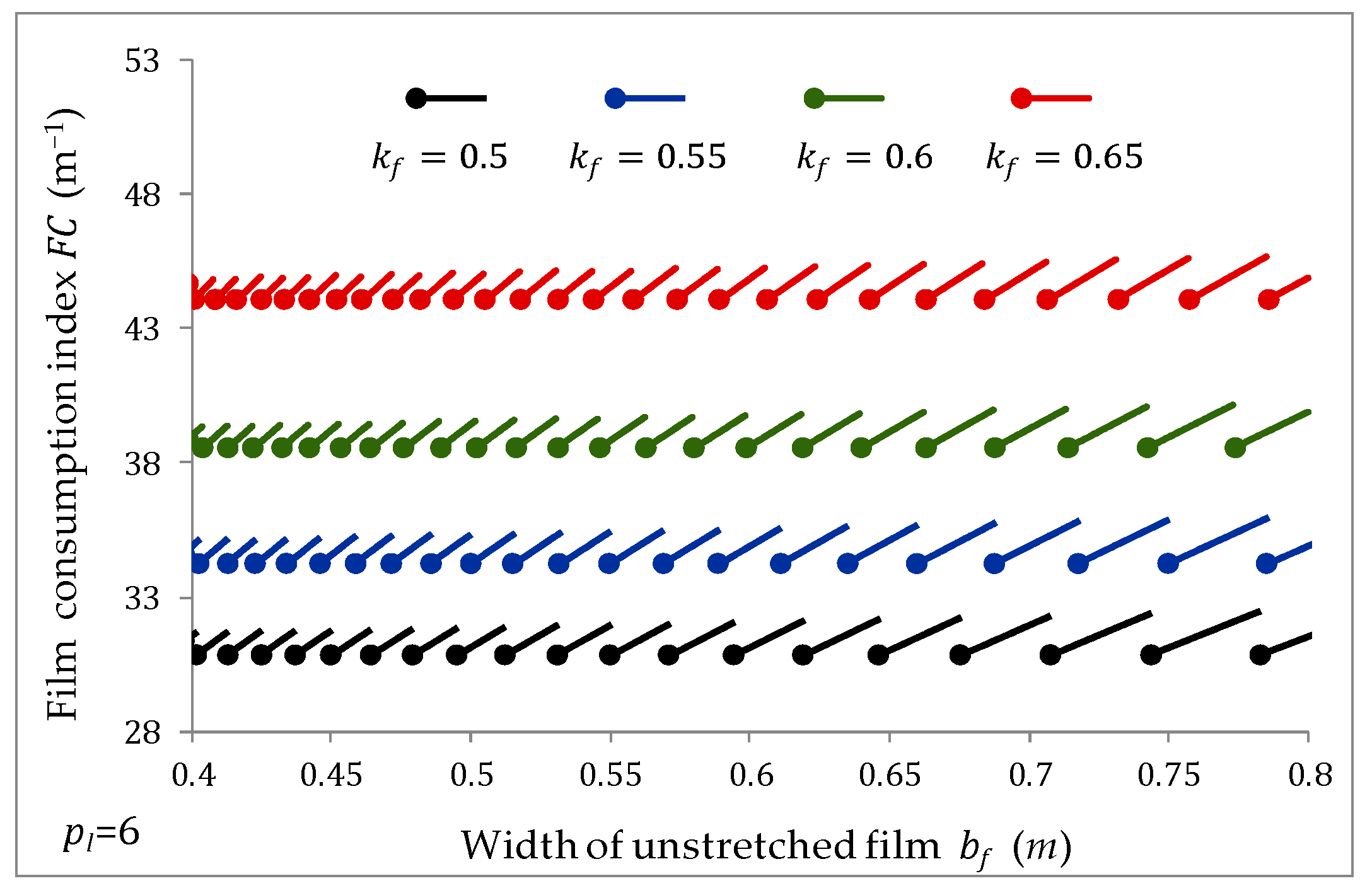
Both every optimal $b_{f,int}$ as well as the optimal $F{C}_{min,b_f}$ described by Equation (11) depend on the overlap ratio, which is evident when comparing the successive columns of Table 1. Figure 5 shows $F{C}_{min,b_f}$ as a function of the ratio $k_f$ for four, six, and eight basic film layers. For $k_f$ variability, according to the applicability condition expressed by Equation (4), the intervals $0<k_f<\frac{2}{3}$ and $\frac{3}{4}\le k_f<\frac{4}{5}$ are chosen for $p_l=4$, and also both applicability intervals $0<k_f<\frac{3}{4}$ and $\frac{5}{6}\le k_f<\frac{6}{7}$ are considered for $p_l=6$. For $p_l=8,$. the ranges $0<k_f<\frac{2}{2}$ and $\frac{3}{4}\le k_f<\frac{4}{5}$ result from the applicability condition; the interval $\frac{7}{8}\le k_f<\frac{8}{9}$ for which this condition is also satisfied is omitted here to make the figure more readable.

3.2. Optimal Design of the Overlap Ratio

Assume now that the film width $b_f$ is given. The subject is to find the overlap ratio such that the film consumption index takes the minimal value. Now, locally, the notation $FC\left(k_f\right),$ indicating the dependence of $FC$ given by Equation (8) on the overlap ratio, is used. Both the ceiling and inside nested floor functions make the function $FC\left(k_f\right)$ hard to analyze. The exemplary course of $FC\left(k_f\right)$ for bale silage from Example 1 is depicted in Figure 6; six film layers and $b_f=0.75\mathrm{m}$ are assumed. For $k_f$ variability, only the interval $0<k_f<\frac{3}{4}$ is considered, according to the applicability condition; the range $\frac{5}{6}\le k_f<\frac{6}{7}$ is omitted here to make the figure more readable.

The index $FC\left(k_f\right)$ is a piecewise-constant function of the ratio $k_f$, which is left-continuous in the discontinuity points $k_{f,int}$, such that:

$$⎡\frac{\pi D_b{p}_l}{2b_f\left(1-v_f{\mathsf{\epsilon }}_{lf}\right)\mathsf{\Omega }\left(k_{f,int}\right)}⎤=\frac{\pi D_b{p}_l}{2b_f\left(1-v_f{\mathsf{\epsilon }}_{lf}\right)\mathsf{\Omega }\left(k_{f,int}\right)},$$

(14)

i.e., the expression under ceiling function brackets in Equation (8) is an integer. It is proven in [21] that under the rationale condition:

$$\pi D_b\ge 2b_f\left(1-v_f{\mathsf{\epsilon }}_{lf}\right)=2b_{fr},$$

(15)

every overlap ratio

$$k_{f,u}=\frac{q-1}{q},$$

(16)

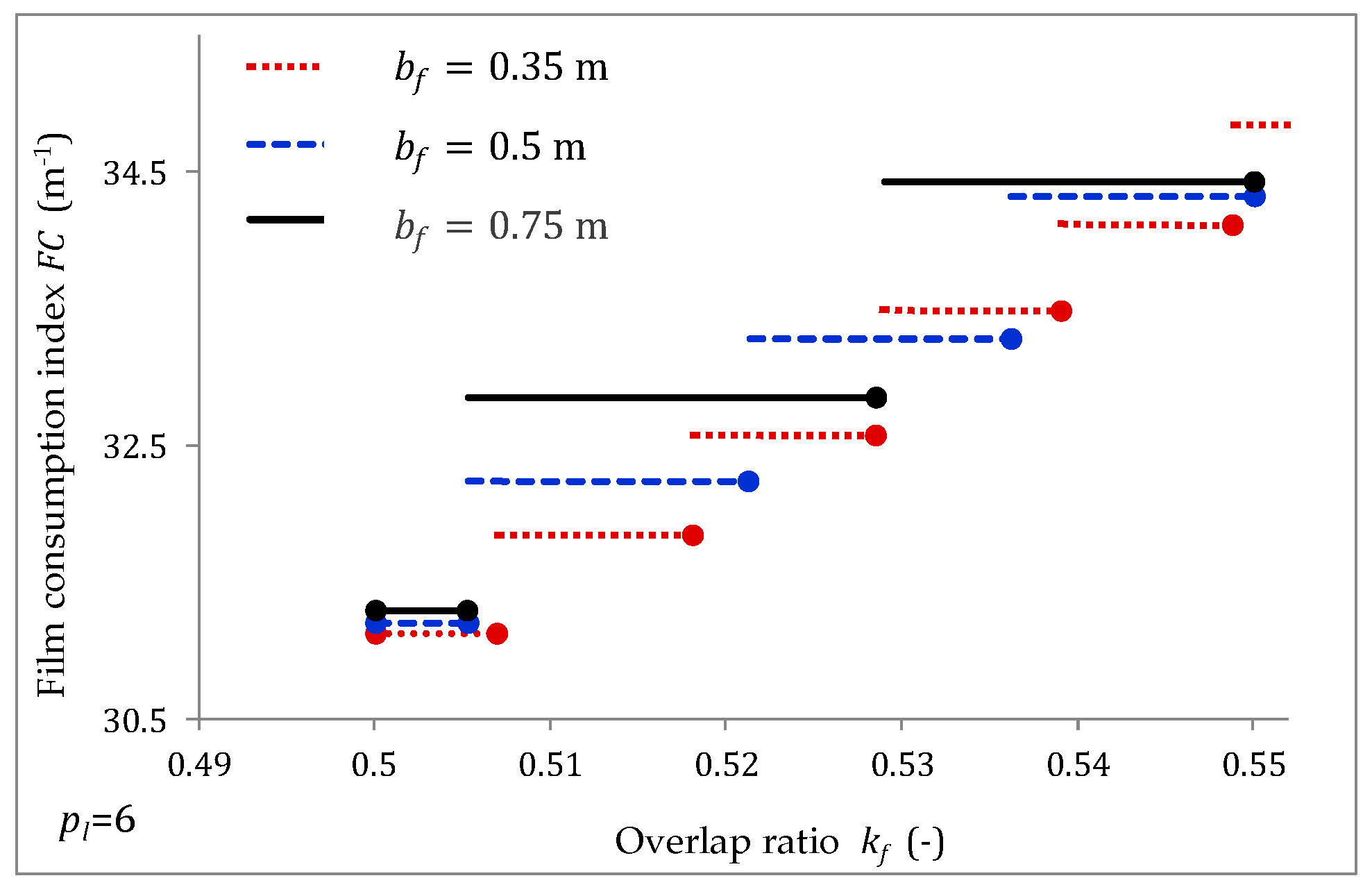
where $q\in \mathcal{N}$, being discontinuity points of $\mathsf{\Omega }\left(k_f\right)$ (see Figure 8 in [21]), is also a discontinuity point of $FC\left(k_f\right)$, in which this function is right-continuous. We denote by ${\mathcal{K}}_u$ the set of all irreducible fractions $k_{f,u}=\frac{1}{2},\frac{2}{3},\frac{3}{4},\dots$ in which the dividend is the divisor minus one. For $k_{f,u}$, the condition expressed by Equation (14) is in general not satisfied. The index $FC\left(k_f\right)$ is a piecewise-constant in the intervals determined by discontinuity points $k_{f,int}$ and a non-decreasing function in the intervals determined by discontinuity points $k_{f,u}$. In any interval defined by two successive $k_{f,u}\in {\mathcal{K}}_u,$ there are many discontinuity points $k_{f,int}$, as shown in Figure 6. The points $k_{f,u}$ are independent of $b_f$, while $k_{f,int}$ are dependent of $b_f$. Figure 7 shows how $b_f$ influences $k_{f,int}$ and better illustrates the piecewise-constant character of $FC\left(k_f\right)$ in the near neighbourhood of $k_{f,u}=\frac{1}{2}$; $FC\left(k_f\right)$ is depicted here for $k_f$ restricted to the interval $0.5\le k_f\le 0.55$ for three popular film widths $b_f=0.35,0.5,\mathrm{and}0.75\mathrm{m}$. As the values of $FC$ are equal in some subintervals, they are slightly differentiated in Figure 7, in order to better illustrate the co-linearity of these subintervals.

Note that for $k_{f,u}\in {\mathcal{K}}_u$ the applicability condition expressed by Equation (4) means that:

$$\frac{p_l}{⎣\frac{1}{1-k_{f,u}}⎦}=\frac{p_l}{q}=m,m\in \mathcal{N},$$

(17)

i.e., that $p_l$ is the multiplicity of integer $q$ uniquely determining the overlap ratio $k_{f,u}$.

In [21], the problem of film area $S_f$, Equation (7), minimization with respect to the overlap ratio is solved. Since $k_f$ does not influence the volume $V_b$ of the bale, the solution of $FC\left(k_f\right)$ minimization task is identical; it is summarized in the next result following directly from Proposition 3 in [21].

Proposition 2.

Assume the bale and film dimensions $D_b$, $H_b$, and $b_f$ are given and are such that the inequality expressed by Equation (15) is satisfied. The solution of the problem of film usage $FC$ minimization with respect to the overlap ratio there exists and is not unique. Let:

$${\chi }_0=\frac{\pi D_b{p}_l}{2b_f\left(1-v_f{\mathsf{\epsilon }}_{lf}\right)},\mathrm{and}$$

(18)

$${\mathsf{\Omega }}_0=\frac{{\mathsf{\chi }}_0}{⎡{\mathsf{\chi }}_0⎤}.$$

(19)

Then:

(i) 

if ${\Omega }_0=1$, then every $k_{f,u}\in {\mathcal{K}}_u$ defined by Equation (16), for which the applicability condition expressed by Equation (17) holds, is an optimal overlap ratio;

(ii) 

if ${\Omega }_0<1$, then for any $k_{f,u}\in {\mathcal{K}}_u$, satisfying the applicability condition from Equation (17) and any $0\le \delta \le {\delta }_0$, where ${\delta }_0$ is defined by:

$${\delta }_0=\frac{1-{\mathsf{\Omega }}_0}{q},$$

(20)

the ratio $k_f=k_{f,u}+\delta$ results in optimal film usage. In both cases the optimal film usage is calculated by:

$$F{C}_{min,k_f}=\frac{8\left(D_b+H_b\right)b_f}{\pi D_b^2{H}_b\left({\mathsf{\epsilon }}_{lf}+1\right)}⎡\frac{\pi D_b{p}_l}{2b_f\left(1-v_f{\mathsf{\epsilon }}_{lf}\right)}⎤.$$

(21)

Note that for the exemplary bale, the inequality expressed by Equation (15) is equivalent to the obvious requirement that $b_f\le 2.0614·D_b$. For an arbitrary $k_{f,u}\in {\mathcal{K}}_u$, the minimal film consumption is reached regardless of the film width value. The optimal film usage $F{C}_{min,k_f}$ is independent of $k_{f,u}$; however, it depends on $b_f$. For the exemplary bale assuming six film layers for $b_f=0.4\mathrm{m},$ we have $F{C}_{min,k_f}=31.6229{\mathrm{m}}^{-1}$, $b_f=0.6\mathrm{m}$ yields $F{C}_{min,k_f}=31.2069{\mathrm{m}}^{-1}$, while $b_f=0.8\mathrm{m}$ results, again, in $F{C}_{min,k_f}=31.6229{\mathrm{m}}^{-1}$.

In view of the above proposition, a natural way to describe this set of the optimal overlap ratios is through the representation of $k_f$ values in the form of closed intervals $\left[k_{f,u},k_{f,u}+{\delta }_0\right]$; Equations (18)–(20) permit us to determine them. For any $k_{f,u}\in {\mathcal{K}}_u,$ if ${\delta }_0>0$, then the ratio $k_{f,u}+{\delta }_0$ is identical to the discontinuity point $k_{f,int}$, which is the nearest right neighbor of $k_{f,u}$ (see Figure 6 and Figure 7). The coefficient ${\chi }_0$, and consequently, also ${\mathsf{\Omega }}_0$ and ${\delta }_0$, depend on the film width. The optimal overlaps are referred to as ${\mathcal{K}}_{b_f}$, which for fixed $b_f$ belongs to the set-sum of intervals $\left[k_{f,u},k_{f,u}+{\delta }_0\right]$ for every $k_{f,u}\in {\mathcal{K}}_u$. Obviously, ${\mathcal{K}}_u\subset {\mathcal{K}}_{b_f}$ for an arbitrary fixed film width. From a practical perspective, however, only four such parameters $k_{f,u}=\frac{1}{2},\frac{2}{3},\frac{3}{4},\frac{4}{5}$ are worth considering; 50%, 67%, and 75% overlaps, especially, are commonly used [5,10,13,14,16]. For a fixed film width, all $k_f\in {\mathcal{K}}_{b_f}$ are equivalent in the sense of optimal film consumption. A simple scheme for determining the set of the optimal overlap ratios, for given film and bale parameters, is presented in [21] (Algorithm 1). It is also proven in [21] that ${\mathcal{K}}_u$ is the complete set of overlap ratios that guarantee uniform film distribution on the lateral surface of the cylindrical bale; however, the applicability condition expressed by Equation (17) must be simultaneously satisfied. Thus, there exists parallelism between the uniform film distribution and minimal film consumption. For any $k_{f,u}\in {\mathcal{K}}_u$ both properties are guaranteed regardless of the dimensions of the bale and film, with or without optimal width. However, the optimal film consumption does not necessarily guarantee the uniform distribution of film layers.

3.3. Optimal Design of the Film Width and Overlap Ratio

Combining the two problems considered above leads to the following task of simultaneous choice of the optimal film width and overlap ratio by solving the following minimization problem:

$$\underset{b_f, k_f}{min} FC\left(b_f,k_f\right)$$

(22)

The notation $FC\left(b_f,k_f\right)$, indicating the dependence of $FC$ on both the film width and the overlap ratio, is used, locally. The goal function $FC\left(b_f,k_f\right)$ is a lower semi-continuous function of both arguments.

In view of Proposition 1, for any fixed overlap ratio, every optimal film width $b_{f,int}$ is defined by Equation (10). The $b_f$-optimal quality index $F{C}_{min,b_f}=FC\left(b_{f,int}\right)$ depends on the overlap ratio $k_f$ according to the formula of Equation (11), as indicated in Figure 5. Since $1/\mathsf{\Omega }\left(k_f\right)$ is the right-continuous function of $k_f$, increasing in the intervals determined by discontinuity points $k_{f,u}\in {\mathcal{K}}_u$, for any $k_{f,u}$ such that the applicability condition holds index $F{C}_{min,b_f}$ takes the minimal value equal to:

$$F{C}_{min}=\frac{4\left(D_b+H_b\right)p_l}{D_b{H}_b\left({\mathsf{\epsilon }}_{lf}+1\right)\left(1-v_f{\mathsf{\epsilon }}_{lf}\right)}.$$

(23)

On the other hand, the results of Proposition 2 state that for any film width $b_f$ being fixed, every $k_f\in {\mathcal{K}}_{b_f}$ satisfying Equation (4), is an optimal overlap ratio, and the optimal film usage $F{C}_{min,k_f}$ is given by Equation (21). This function is minimal if and only if the film width $b_{f,0}$ is such that:

$$\frac{\pi D_b{p}_l}{2b_{f,0}\left(1-v_f{\mathsf{\epsilon }}_{lf}\right)}=\frac{\pi D_b{p}_l}{2b_{f,0}\left(1-v_f{\mathsf{\epsilon }}_{lf}\right)}.$$

(24)

Substituting Equation (24) into Equation (21) gives the optimal $F{C}_{min}$, Equation (23). Thus, we have $F{C}_{min,k_f}\left(b_{f,0}\right)=F{C}_{min}$. For brevity, we denote by ${ℬ}_0$ the set of all $b_{f,0}$ in the range of practically meaningful film widths, for which Equation (24) is satisfied. Note that Equation (24) is, in fact, Equation (10), for $k_f=k_{f,u}$. Since for an arbitrary $b_{f,0}$ the coefficient ${\chi }_0$ given by Equation (18) is an integer, thus ${\mathsf{\Omega }}_0=1$ and Equation (20) yield ${\delta }_0=0$. The set ${\mathcal{K}}_{b_{f,0}}$ of optimal overlap ratios reduces to ${\mathcal{K}}_u$, i.e., for optimal film width $b_{f,0}$ only the overlap ratios $k_{f,u}$ result in minimal film usage. The next result is valid.

Proposition 3.

Assume the bale dimensions $D_b$ and $H_b$ and the number of film layers $p_l$ are given. The solution of the film consumption minimization task stated in Equation (22) there exists and is not unique. Every $k_{f,u}\in {\mathcal{K}}_u$, for which the applicability condition expressed by Equation (17) is satisfied, is the optimal overlap ratio; ${ℬ}_0$ is the set of optimal widths of un-stretched film. The optimal film consumption $F{C}_{min}$ is given by Equation (23).

Since for every $b_{f,0}\in {ℬ}_0$ the ratio ${\chi }_0$ introduced by Equation (18) is an integer, by Equations (5), (18) and (24) we have:

$$i_f={\chi }_0=\frac{\pi D_b{p}_l}{2b_{f,0}\left(1-v_f{\epsilon }_{lf}\right)};$$

(25)

thus, every $b_{f,0}$ can be expressed as:

$$b_{f,0}=\frac{\pi D_b{p}_l}{2i_f\left(1-v_f{\epsilon }_{lf}\right)}=\frac{\pi D_b{p}_l}{2{\chi }_0\left(1-v_f{\epsilon }_{lf}\right)}.$$

(26)

Thus, similar to the separate problem of the optimal film width selection, the relation between $b_{f,0}$ and the resulting number of entire film wrappings $i_f={\chi }_0$ is described by Equation (25) or, equivalently, by Equation (26). From the computational point of view, the formula given by Equation (26) is more useful than directly solving the definitional Equation (24).

In view of the above proposition, only exact $k_{f,u}$ and the film widths $b_{f,0}$ are, simultaneously, optimal. However, even the smallest disturbance in any of the wrapping process parameters may result in the loss of the optimality. In particular, an overlap ratio other than the assumed may result from inaccuracies in the functioning of the wrapper. From a mathematical perspective, such variability entails uncertainty in the overlap ratio. The following section addresses some robustness issues.

3.4. Robustness

As we ascertained above, for any optimal $b_{f,0}\in {ℬ}_0$, only the overlaps $k_{f,u}$ result in optimal film consumption. Thus, the optimal $b_{f,0}$ does not provide any robustness to overlap ratio variations. A non-optimal $b_f$, for which ${\delta }_0>0$, implies the non-one-point intervals of optimal overlaps $\left[k_{f,u},k_{f,u}+{\delta }_0\right]$ for every applicable $k_{f,u}\in {\mathcal{K}}_u$. Both larger than $k_{f,u}+{\delta }_0$ as well as smaller than $k_{f,u}$ overlap ratios imply the growth of film consumption. Thus, the length of this interval, which is estimated by ${\delta }_0$, can be treated as a measure of robustness to parameter uncertainty—robustness margin [21]. The larger ${\delta }_0$ is, the greater robustness with respect to $k_f$ uncertainty is achieved. For the exemplary bale and a few widths of the film, the robustness margins ${\delta }_0$ are shown in

Table 3. The lengths ${\delta }_0$ of the intervals of the optimal overlap ratios (robustness margins) for $p_l=2,\dots ,10$ pre-assumed film layers.

The Lengths ${\mathit{\delta }}_0$ of the Intervals $\left[{\mathit{k}}_{\mathit{f},\mathit{u}}, {\mathit{k}}_{\mathit{f},\mathit{u}}+{\mathit{\delta }}_0\right]$ of Optimal Overlap Ratios $\left(\mathbf{m}\right)$
${\mathit{k}}_{\mathit{f},\mathit{u}}$	${\mathit{b}}_{\mathit{f}}=0.4 \mathbf{m}$	${\mathit{b}}_{\mathit{f}}=0.5 \mathbf{m}$	${\mathit{b}}_{\mathit{f}}=0.6 \mathbf{m}$	${\mathit{b}}_{\mathit{f}}=0.7 \mathbf{m}$	${\mathit{b}}_{\mathit{f}}=0.7067 \mathbf{m}$	${\mathit{b}}_{\mathit{f}}=0.75 \mathbf{m}$	${\mathit{b}}_{\mathit{f}}=0.8 \mathbf{m}$
$p_l=2$ film layers
$\frac{1}{2}$	0.02429	0.00526	0.04191	0.05827	0.06246	0.02882	0.05827
$p_l=3$ film layers
$\frac{2}{3}$	0.00785	0.00351	0.01619	0.01207	0.01512	0.00351	0.02412
$p_l=4$ film layers
$\frac{1}{2}$	0.00526	0.00526	0.01496	0.02882	0.03329	0.02882	0.02429
$\frac{3}{4}$	0.00263	0.00263	0.00748	0.01441	0.01664	0.01441	0.01215
$p_l=5$ film layers
$\frac{4}{5}$	0.00051	0.0021	0.00368	0.00367	0.00554	0.00598	0.00674
$p_l=6$ film layers
$\frac{1}{2}$	0.01177	0.00526	0.00526	0.01811	0.02268	0.00526	0.01177
$\frac{2}{3}$	0.00785	0.00351	0.00351	0.01207	0.01512	0.00351	0.00785
$\frac{5}{6}$	0.00392	0.00175	0.00175	0.00604	0.00756	0.00175	0.00392
$p_l=7$ film layers
$\frac{6}{7}$	0.00231	0.0015	0.00069	0.0015	0.00284	0.00543	0.0023
$p_l=8$ film layers
$\frac{1}{2}$	0.00526	0.00526	0.00026	0.01257	0.01719	0.01137	0.00526
$\frac{3}{4}$	0.00263	0.00263	0.00013	0.00627	0.0086	0.00568	0.00263
$\frac{7}{8}$	0.00132	0.00132	6.591E-05	0.00314	0.0043	0.00284	0.00132
$p_l=9$ film layers
$\frac{2}{3}$	0.002	0.0035	0.00785	0.002	0.0052	0.0035	0.002
$p_l=10$ film layers
$\frac{1}{2}$	0.00127	0.00526	0.00919	0.00919	0.01384	0.00026	0.00127
$\frac{4}{5}$	0.0005	0.0021	0.00367	0.00367	0.00554	0.0001	0.0005

for two to ten pre-assumed film layers. Mostly, four, six, or eight layers of film are applied [5,14,31]; however, two, 10, and even 16 film layers in which the silages are wrapped have also been considered [22,31]. Naturally, only $k_{f,u}\in {\mathcal{K}}_u$, which satisfies the applicability condition, Equation (17), for a given $p_l,$ is considered. The formula from Equation (20) means that the smaller $q$ is, i.e., the smaller $k_{f,u}$ is, the bigger the resulting robustness margin is. This rule can be confirmed by an inspection of data in the columns of Table 3, for any fixed $p_l$, separately. Increasing $k_{f,u}$ reduces the lengths of the intervals of optimal overlap ratios. However, the difference between $k_{f,u}$ and subsequent ${\overline{k}}_{f,u}\in {\mathcal{K}}_u$, equal to $\frac{1}{q\left(q+1\right)}$, also decreases for an increasing $k_{f,u}$.

The selection of the film width $b_f$ and the respective overlap ratio, to guarantee the best robustness on $k_f$ uncertainty, is now the subject of interest. For fixed $k_{f,u}$ the robustness margin ${\delta }_0$ depends on the film width. By Equations (18)–(20), we have:

$${\delta }_0=\frac{1}{q}\left[1-\frac{1}{\frac{2b_f\left(1-v_f{\epsilon }_{lf}\right)}{\pi D_b{p}_l}⎡\frac{\pi D_b{p}_l}{2b_f\left(1-v_f{\epsilon }_{lf}\right)}⎤}\right],$$

(27)

where we conclude that ${\delta }_0$ is a semi-continuous increasing right-continuous function of the film width $b_f$ in the intervals determined by discontinuity points $b_{f,0}$, Equation (24). The margin ${\delta }_0$ is illustrated by Figure 8, where ${\delta }_0$ is depicted as a function of $b_f$ for three overlap ratios $k_{f,u}$. The upper bound ${\overline{\delta }}_0$ of ${\delta }_0$ for the range $b_{f,0}\le b_f<{\overline{b}}_{f,0}$, where ${\overline{b}}_{f,0}$ is a direct successor of $b_{f,0}$ in the set ${ℬ}_0$, results immediately as the left-hand sided limit:

$${\overline{\delta }}_0=\underset{{b_f\to {\overline{b}}_{f,0}}^{-}}{lim}{\delta }_0=\frac{2b_{f,0}\left(1-v_f{\epsilon }_{lf}\right)}{\pi D_b{p}_{l}q};$$

(28)

for derivation see Appendix A.1. Thus, the larger $b_{f,0}$ is, the longer the interval of $k_f$-optimal overlap ratios may be, if the width of the film is chosen in the nearest left neighborhood of ${\overline{b}}_{f,0}$. The above rules are also illustrated in Figure 8.

3.5. Robustly Optimal Design of Wrapping Parameters

The optimal film usage is never achieved if $b_f\notin {ℬ}_0$. Other than $b_{f,0}$, film width means a larger than optimal $F{C}_{min}$ film consumption, even if the overlap ratio is optimal; however, the robustness is guaranteed in such a case. The selection of the best commercially available film width is resolved by the following result proven in Appendix A.2. In various regions of the world, different film widths dominate (see, e.g., [11]). Both the film consumption and the robustness with respect to the overlap ratio uncertainties are taken into account.

Proposition 4.

Let ${ℬ}_f$ be the set of all considered film widths that may be commercially available. Assume ${\overline{b}}_{f,0}>b_{f,0}$ is the direct successor of $b_{f,0}$ in the set ${ℬ}_0$. Let:

$$b_{f,s}=b_{f,0}+\Delta b_f,$$

(29)

where $b_{f,s}\in {ℬ}_f$ is commercially available width of the film such that:

$$b_{f,0}\le b_{f,s}<{\overline{b}}_{f,0}.$$

(30)

Then:

(i) 

The $k_f$-optimal film consumption index $F{C}_{min,k_f}$ expressed by Equation (21) takes the minimal value in the set ${ℬ}_f$ if and only if the quotient:

$$\frac{\Delta b_f}{b_{f,0}}=\frac{b_{f,s}-b_{f,0}}{b_{f,0}},$$

(31)

is minimal in the set ${ℬ}_f$. The increase of the index $F{C}_{min,k_f}$:

$$\Delta F{C}_{min,k_f}\left(b_{f,s}\right)=F{C}_{min,k_f}\left(b_{f,s}\right)-F{C}_{min},$$

(32)

is described by:

$$\Delta F{C}_{min,k_f}\left(b_{f,s}\right)=F{C}_{min}·\frac{\Delta b_f}{b_{f,0}}.$$

(33)

(ii) 

For $b_{f,s}\in \left({ℬ}_f-{ℬ}_0\right)$ the length ${\delta }_0$ of the interval of overlap ratios ensuring $k_f$ -optimal film usage is given by:

$${\delta }_0=\frac{1}{q}·\frac{1}{\frac{b_{f,0}}{\Delta b_f}+1}.$$

(34)

The length ${\delta }_0$ takes the maximal value in the set ${ℬ}_f$ if and only if the quotient $\Delta b_f/b_{f,0}$ is maximal in ${ℬ}_f$.

By the above proposition, the requirements concerning minimal film usage and significant robustness are not consistent. To choose $b_{f,s}\in {ℬ}_f$ the compromise is necessary, which must be resolved on a case by case basis having in mind both the value of ${\mathsf{\delta }}_0$ and the relative percentage error, calculated by the following:

$$ERR=\frac{\Delta F{C}_{min,k_f}\left(b_{f,s}\right)}{F{C}_{min}}·100\%=\frac{\Delta b_f}{b_{f,0}}·100\%.$$

(35)

Proposition 4 clearly shows that the quotient $\Delta b_f/b_{f,0}$ is significant to synthesis of the algorithm for optimal and robust design of the wrapping parameters. This quotient allows one to choose the best film width $b_{f,s}\in {ℬ}_f$, estimate the film consumption deterioration according to formula from Equation (33), and also enable easy determination of both the robustness margin ${\delta }_0$, as characterized by Equation (34), and the relative error given by Equation (35), on the basis of which the overlap ratio is chosen according to the design scheme presented below.

3.6. Algorithm

(1)

Take initially $k_{f,u}=\left(q-1\right)/q$ such that the applicability condition expressed by Equation (17) is fulfilled, i.e., $p_l/q$ is an integer.

(2)

For any commercially available $b_{f,s}\in {ℬ}_f$ find optimal $b_{f,0}\in {ℬ}_0$ being the nearest lower neighbours of $b_{f,s}$ using the direct formula from Equation (26) or solving Equation (24).

(3)

If a $b_{f,s}$ is identical to $b_{f,0}$, then reject this $b_{f,s}$ from consideration, i.e., consider only $b_{f,s}\in \left({ℬ}_f-{ℬ}_0\right)$.

(4)

For any pair $\left(b_{f,s},b_{f,0}\right)$ compute the quotient $\Delta b_f/b_{f,0}$ according to Equation (31), and next estimate robustness margin ${\mathsf{\delta }}_0$ according to Equation (34).

(5)

Select such $b_{f,s}$ for which both respective robustness margin ${\mathsf{\delta }}_0$ and the relative error of film consumption described by Equation (35) are satisfactory.

(6)

Choose the overlap ratio from inside of the interval $\left[k_{f,u},k_{f,u}+{\delta }_0\right]$, e.g., $k_f=k_{f,u}+\frac{{\delta }_0}{2}$.

By Equations (27) and (34), the overlap ratio $k_{f,u}=\frac{1}{2}$, which means that $q=2$, can be recommended to maximize the robustness margin. In this case the applicability condition is fulfilled for any even $p_l$. Now, on the basis of the quotient $\Delta b_f/b_{f,0}$, this $b_{f,s}\in {ℬ}_f$ for which the film consumption $F{C}_{min,k_f}$ is minimal, or such that the margin ${\delta }_0$ is maximal, or such that the trade-off between these requirements is achieved, can be chosen. The following example illustrates the use of Proposition 4 and motivates the above algorithm for wrapping parameter robust design. The example is also aimed at illustrating the process of the best film width selection.

Example 2

The bale from the previous example is considered; bale height $H_b=1.2$ m is assumed [5], and $k_f=k_{f,u}=\frac{1}{2}$ is taken together with $p_l=4,6,8,10$ for film wrapping layers. We assume that the film widths $b_{f,s}\in {ℬ}_f$, given in the second column of

Table 4. The optimal $b_{f,0}$ and commercially available $b_{f,s}$ widths of un-stretched film, the quotient $\frac{\Delta b_f}{b_{f,0}}$ Equation (31), the robustness margin ${\delta }_0$ Equation (27), $F{C}_{min,k_f}\left(b_{f,s}\right)$ ($k_f$–optimal film consumption), sided estimations of $F{C}_{min,k_f}\left(b_{f,s}\right)$, left-hand $F{C}_L\left(b_{f,s}\right)$ Equation (36), right-hand $F{C}_R\left(b_{f,s}\right)$ Equation (37), the relative errors $ERR$, Equation (35); $k_{f,u}=\frac{1}{2}$, $p_l=4,6,8,10$.

${\mathit{b}}_{\mathit{f},0} \left(\mathbf{m}\right)$	${\mathit{b}}_{\mathit{f}, \mathit{s}} \left(\mathbf{m}\right)$	$\frac{\mathit{\Delta }{\mathit{b}}_{\mathit{f}}}{{\mathit{b}}_{\mathit{f},0}}$	${\mathit{\delta }}_0 (-)$	$\mathit{F}{\mathit{C}}_{\mathit{m}\mathit{i}\mathit{n},{\mathit{k}}_{\mathit{f}}}{\left({\mathit{b}}_{\mathit{f},\mathit{s}}\right)}_{}$	$\mathit{F}{\mathit{C}}_{\mathit{L}}\left({\mathit{b}}_{\mathit{f},\mathit{s}}\right)$	$\mathit{F}{\mathit{C}}_{\mathit{R}}\left({\mathit{b}}_{\mathit{f},\mathit{s}}\right)$	$\mathit{E}\mathit{R}\mathit{R} (\%)$
$p_l=4$ film layers
0.39579	0.4	0.01063	0.00526	20.80457	41.60914	21.637	1.063
0.44976	0.45	0.00053	0.00026	20.59652	41.19304	21.533	0.053
0.49474	0.5	0.01064	0.00526	20.80457	41.60914	21.845	1.064
0.54971	0.55	0.00053	0.00026	20.59652	41.19304	21.741	0.053
0.58205	0.6	0.03085	0.01496	21.22066	41.19304	22.469	3.085
0.61842	0.65	0.05106	0.02429	21.63675	41.9212	22.989	5.106
0.65965	0.7	0.06116	0.02882	21.8448	42.23327	23.301	6.116
0.70677	0.75	0.06116	0.02882	21.8448	42.12925	23.405	6.116
0.76114	0.8	0.05106	0.02429	20.59652	41.60914	23.301	5.106
$p_l=6$ film layers
0.39058	0.4	0.02411	0.01177	31.62294	62.4137	32.455	2.411
0.44976	0.45	0.00053	0.00026	30.8948	61.78957	31.83099	0.053
0.49474	0.5	0.01063	0.00526	31.20685	62.41370	32.24708	1.063
0.54971	0.55	0.00053	0.00026	30.89478	61.78957	32.0390	0.053
0.59369	0.6	0.01063	0.00526	31.20685	62.41370	32.45513	1.063
0.64531	0.65	0.00726	0.00361	31.10283	62.20566	32.45513	0.726
0.67464	0.7	0.03758	0.01811	32.03903	62.62175	33.49535	3.758
0.74211	0.75	0.01063	0.00526	31.20685	62.41370	32.76719	1.063
0.78117	0.8	0.02411	0.01177	31.62294	63.24589	33.28731	2.411
$p_l=8$ film layers
0.39579	0.4	0.01064	0.00526	41.60914	82.38609	42.441	1.064
0.44976	0.45	0.00053	0.00026	41.19304	82.38609	42.129	0.053
0.49474	0.5	0.01063	0.00526	41.60914	83.21827	42.649	1.063
0.54971	0.55	0.00053	0.00026	41.19304	82.38609	42.337	0.053
0.59968	0.6	0.00053	0.00026	41.19304	82.38609	42.441	0.053
0.63837	0.65	0.01821	0.00894	41.9212	82.49011	43.274	1.821
0.68239	0.70	0.02579	0.01257	42.23327	83.01023	43.69	2.579
0.73295	0.75	0.02327	0.01137	42.12925	82.69816	43.69	2.327
0.79158	0.8	0.01063	0.00526	41.60914	83.21827	43.274	1.063
$p_l=10$ film layers
0.39898	0.4	0.00255	0.00127	51.59533	103.1907	52.428	0.255
0.44976	0.45	0.00053	0.00026	51.49131	102.9826	52.428	0.053
0.49474	0.5	0.01063	0.00526	52.01142	102.9826	53.052	1.063
0.54971	0.55	0.00053	0.00026	51.49131	102.9826	52.636	0.053
0.58897	0.6	0.01872	0.00919	52.42751	103.6067	53.676	1.872
0.63428	0.65	0.02478	0.01209	52.73958	104.1269	54.092	2.478
0.68714	0.70	0.01872	0.00919	52.42751	103.3987	53.884	1.872
0.74960	0.75	0.00053	0.00026	51.49131	102.9826	53.052	0.053
0.79797	0.8	0.00255	0.00127	51.59533	103.1907	53.26	0.255

The values marked by bold correspond to the minimal film consumption or maximal robustness margin and are discussed in Example 2.

, are integer multiples of 5 cm from the range $0.4\le b_{f,s}\le 0.8 \mathrm{m}$. Since $k_f=\frac{1}{2}\in {\mathcal{K}}_u$, the film widths $b_{f,int}$ and $b_{f,0}$ are identical for any fixed $p_l$; they depend on the number of film layers. In the range from $0.4$ to $0.8$ m for $p_l=4$, there are 12 optimal film widths; for $p_l=6$ nineteen $b_{f,int}=b_{f,0}$ are given in the first column of Table 1, while for $p_l=8$ in this range, there are 25 optimal film widths, and for $p_l=10$ there are as many as 31 $b_{f,0}$. For any $p_l$ there are only nine values of $b_{f,0}$ such that the inequalities expressed in Equation (30) hold, and only these $b_{f,0}$, which are necessary to estimate the quotient $\Delta b_f/b_{f,0}$, Equation (31), are given in Table 4 for $p_l=4,6,8,\mathrm{and}10$. Furthermore, in the first row, the largest $b_{f,0}$ smaller than $0.4 \mathrm{m}$ are specified in order to estimate $\Delta b_f/b_{f,0}$ for $b_{f,s}=0.4 \mathrm{m}$. The quotients $\Delta b_f/b_{f,0}$ are given in the third column in Table 4, where also the robustness margins ${\delta }_0$ and the indices $F{C}_{min,k_f}\left(b_{f,s}\right)$ are added. Additionally, the left-hand sided limits (for derivation, see Appendix A.3) are as follows:

$$F{C}_L\left(b_{f,s}\right)=\underset{{k_f\to k_{f,u}}^{-}}{lim}FC\left(k_f\right)=\frac{8\left(D_b+H_b\right)b_{f,s}}{\pi D_b^2{H}_b\left({\epsilon }_{lf}+1\right)}⎡\frac{\pi D_b{p}_{l}q}{2b_{f,s}\left(1-v_f{\epsilon }_{lf}\right)\left(q-1\right)}⎤,$$

(36)

where $q=2$, which characterize the film consumption if the actual overlap ratio $k_f$ is smaller than the assumed $k_{f,u}=\frac{1}{2}$. The right-hand sided limits of film consumption, expressed as:

$$F{C}_R\left(b_{f,s}\right)=\underset{k_f\to {\left(k_{f,u}+{\delta }_0\right)}^{+}}{lim}FC\left(k_f\right)=FC\left({\overline{k}}_{f,int}\right),$$

(37)

which are also given in Table 4. Here, ${\overline{k}}_{f,int}$ is the direct successor of $k_{f,int}=k_{f,u}+{\delta }_0$ in the set of overlap ratios satisfying Equation (14) for $b_{f,s}$. The limit defined by Equation (37) characterizes the film usage, if the actual overlap $k_f$ is greater than $k_{f,u}+{\delta }_0$. In the last column, the errors $ERR$, Equation (35), are given. The globally optimal film consumptions are as follows: for $p_l=4$ we have $F{C}_{min}=20.58566{\mathrm{m}}^{-1}$, for $p_l=6$ the respective $F{C}_{min}=30.87849{\mathrm{m}}^{-1}$, $p_l=8$ film layers means $F{C}_{min}=41.17132{\mathrm{m}}^{-1}$, while $p_l=10$ entails $F{C}_{min}=51.46415{\mathrm{m}}^{-1}$.

By an inspection of the third column data in Table 4, it is evident that for all the considered numbers of film layers, there are two film width, $b_{f,s}=0.45\mathrm{m}$ and $b_{f,s}=0.55\mathrm{m}$, for which the quotient $\Delta b_f/b_{f,0}$ is minimal, i.e., minimal film consumption is achieved. For $p_l=8,$ $b_{f,s}=0.6\mathrm{m}$ also results in minimal $\Delta b_f/b_{f,0}$, while for $p_l=10,$ this minimum is also achieved for $b_{f,s}=0.75\mathrm{m}$. In all these cases, $ERR\cong 0.053\%$.

The maximal robustness margin ${\delta }_0$ is guaranteed by $b_{f,s}=0.7\mathrm{m}$ for $p_l=4,6,\mathrm{and}8$, while for $p_l=10$, the film width $b_{f,s}=0.65\mathrm{m}$ results in the maximal $\Delta b_f/b_{f,0}$. For $p_l=4$ the popular film width $b_{f,s}=0.75\mathrm{m}$ [12,14] also yields the maximal ${\delta }_0$. The maximal robustness margin for $p_l=4$ implies an increase of film consumption measured by $ERR=6.1165\%$, while for the other numbers of basic film layers this error is smaller than $3.76\%$.

From these data, it follows, for example, that if $ERR\le 5\%$ and robustness margin ${\delta }_0\ge 0.02$ are assumed in the case of $p_l=4,$ there are no practically accessible film widths satisfying these requirements, while for $b_{f,s}=0.8\mathrm{m},$ the respective $ERR=5.105\%$ slightly exceeds the assumed level. For $p_l=6,8,10,$ the errors are such that $ERR\le 4\%$; however, none of the film widths $b_{f,s}\in {ℬ}_f$ ensure the pre-assumed robustness margin. Subsequently, $ERR\le 4\%$ and ${\delta }_0\ge 0.01$ are assumed. Now, a recommendation for the film width based on the data states that a well-chosen $b_{f,s}$ for $p_l=4$ can be $b_{f,s}=0.6\mathrm{m}$; for $p_l=6$ there are three acceptable film widths, $b_{f,s}=0.4,0.7,\mathrm{and}0.8\mathrm{m}$, of which $b_{f,s}=0.7\mathrm{m}$ results in the maximal robustness margin. Two film widths, $b_{f,s}=0.7\mathrm{and}0.75\mathrm{m},$ are acceptable for $p_l=8$ and only one, $b_{f,s}=0.65\mathrm{m},$ seems to be acceptable for $p_l=10$. Note that model-based simulations like this are helpful in understanding more deeply the impact of the model variables and parameters on film usage.

3.7. Error Analysis

Taking into account the inequalities expressed by Equations (29) and (30), the increase $\Delta b_f$ can be bounded as follows:

$$\Delta b_f<{\overline{b}}_{f,0}-b_{f,0},$$

(38)

where, by Equation (26) and an analogous equation describing ${\overline{b}}_{f,0}$:

$${\overline{b}}_{f,0}=\frac{\pi D_b{p}_l}{2\left(i_f-1\right)\left(1-v_f{\mathsf{\epsilon }}_{lf}\right)},$$

which also results directly from Equation (A3), the distance:

$${\overline{b}}_{f,0}-b_{f,0}=\frac{\pi D_b{p}_l}{2\left(i_f-1\right)i_f\left(1-v_f{\epsilon }_{lf}\right)}.$$

(39)

Having in mind Equation (26) and the last expression in Equation (35), we see that the following upper bound holds:

$$ERR=\frac{\Delta b_f}{b_{f,0}}·100\%<\frac{1}{i_f-1}·100\%=ER{R}_u,$$

(40)

which means that the bigger $i_f$ is, i.e., the smaller $b_{f,s}$ and the bigger $p_l$ are, the smaller error $ERR$ for the film width $b_{f,s}$ may arise. Simultaneously, by Equation (39), decreasing $b_{f,s}$ and increasing $p_l$ reduces the distance between successive discontinuity points, $b_{f,0}$ and ${\overline{b}}_{f,0}$, from which the estimation $ER{R}_u$ resulting from inequality expressed in Equation (38) is closer (more accurate) for smaller $b_{f,s}$. These rules can be confirmed by an inspection of data in

Table 5. The upper bounds $ER{R}_u$ defined in Equation (40) of the relative errors $ERR$ Equation (35), for the commercially available film widths $b_{f,s}$ of un-stretched film for $p_l$ film layers.

The Upper Bounds $\mathit{E}\mathit{R}{\mathit{R}}_{\mathit{u}}$ of the Relative Errors $\mathit{E}\mathit{R}\mathit{R}$
${\mathit{b}}_{\mathit{f},\mathit{s}} \left(\mathbf{m}\right)$	${\mathit{p}}_{\mathit{l}}$
	3	4	5	6	8	9	10	12	14	15	16
0.4	5.556	4.167	3.333	2.703	2.041	1.818	1.639	1.351	1.163	1.087	1.020
0.45	6.250	4.762	3.704	3.125	2.326	2.041	1.852	1.538	1.316	1.220	1.149
0.5	7.143	5.263	4.167	3.448	2.564	2.273	2.041	1.695	1.449	1.351	1.266
0.55	7.692	5.882	4.545	3.846	2.857	2.500	2.273	1.887	1.587	1.493	1.408
0.6	8.333	6.250	5.000	4.167	3.125	2.703	2.381	2.041	1.754	1.639	1.538
0.65	9.091	6.667	5.263	4.545	3.333	2.941	2.632	2.222	1.887	1.754	1.667
0.70	10.0	7.143	5.882	4.762	3.571	3.226	2.857	2.381	2.041	1.887	1.786
0.75	11.111	7.692	6.250	5.263	3.846	3.448	3.125	2.564	2.174	2.041	1.923
0.8	11.111	8.333	6.667	5.556	4.167	3.704	3.333	2.703	2.326	2.174	2.041

, where the upper bounds $ER{R}_u$ are given for three to 16 film layers, which are reachable for the first five overlap ratios $k_{f,u}\in {\mathcal{K}}_u$, i.e., for which the applicability condition expressed by Equation (17) holds, and $0.4\le b_{f,s}\le 0.8 \mathrm{m}$ being an integer multiple of 5 cm. Note that for $p_l\ge 9$ not only the original $ERR$, but also its upper bound do not exceed 4%.

4. Discussion

As previously stated, disturbance in the functioning of an actual bale wrapper is the main justification for robustness studies. In view of Equation (A5), which can be rewritten as:

$${\delta }_0=\frac{1}{q}\left[1-\frac{b_{f,0}}{b_{f,0}+\Delta b_f}\right],$$

there is greater tolerance to overlap ratio uncertainty when the film width is increased between $b_{f,0}$ and its successor in the set ${ℬ}_0$ of optimal film widths. Increasing the overlap above $k_{f,u}+{\delta }_0$ or decreasing them below $k_{f,u}$ causes a loss of optimality, even for very small uncertainties. A value smaller than $k_{f,u}$ may lead, especially for $k_{f,u}=\frac{1}{2}$, to dramatically big increases in film usage, which is estimated and characterized by the left-hand sided limit $F{C}_L\left(b_{f,s}\right)$ described in Equation (36). The values of $F{C}_L\left(b_{f,s}\right)$ given for the commercially available $b_{f,s}$ in Table 4 for $k_{f,u}=\frac{1}{2}$ are more than twice as large as $F{C}_{min}$ and almost twice as $F{C}_{min,k_f}$ for respective film widths, regardless of the number of film layers. It may be observed that the bigger $k_{f,u}$ is, the smaller the increase in film consumption is, if the overlap ratio decreases below $k_{f,u}$. For $k_{f,u}=\frac{2}{3}$ the limit $F{C}_L\left(b_{f,s}\right)$ is about one and a half times bigger than $F{C}_{min}$ and $F{C}_{min,k_f}$. Additionally, Figure 6 shows how the overlap ratio uncertainty in the near left-neighborhood of an arbitrary $k_{f,u}$ influences film consumption. Simultaneously, the robustness margin ${\delta }_0$ is reduced for larger $k_{f,u}$. A quick inspection of the data in Table 4 also leads to the conclusion that a small increase of the overlap ratio above the right margin $k_{f,u}+{\delta }_0$ of the ‘optimality’ interval results in significantly smaller increases in film usage, because the right-hand sided limit $F{C}_R\left(b_{f,s}\right)$, Equation (37), is such that $1.05\le \vartheta \le 1.078$ for $p_l=6$, where the ratio is:

$$\vartheta =\frac{F{C}_R\left(b_{f,s}\right)}{F{C}_{min,k_f}\left(b_{f,s}\right)}.$$

For $p_l=4$, this ratio is characterized by $1.04\le \vartheta \le 1.0769$; for $p_l=8$ and $p_l=10,$ the estimations are $1.02\le \vartheta \le 1.04$ and $1.016\le \vartheta \le 1.032$, respectively. Thus, paradoxically, optimal parameters $k_{f,u}\in {\mathcal{K}}_u$ may lead to dramatically unfavorable film consumption if any disturbance appears, which, therefore, must be absolutely avoided, while near-optimal parameters, not much bigger than $k_{f,u}+{\delta }_0$, may result in almost optimal film usage. Both the reported properties suggest that, since the intervals of optimal overlap ratios contain only the right neighborhood of $k_{f,u}$, it is reasonable to take $k_{f,u}+{\delta }_0$, rather than the exact $k_{f,u}$, or such overlaps that belong to the interior of the interval $\left[k_{f,u},k_{f,u}+{\delta }_0\right]$, as in the Algorithm.

Proposition 4 demonstrates that the optimal and robust design of the film width and overlap ratio generally lead to conflicting requirements. Based on the results of numerical studies conducted for the exemplary bale, as seen in

Table 6. The minimal film consumption or maximal robustness margins ${\delta }_0$ attainable for the commercially available film widths $b_{f,s}$ of un-stretched film (marked by the sign ‘x’) for $p_l$ film layers.

The Minimal Film Consumption									Maximal Robustness Margin
${\mathit{b}}_{\mathit{f},\mathit{s}} \left(\mathbf{m}\right)$	${\mathit{p}}_{\mathit{l}}$								${\mathit{p}}_{\mathit{l}}$
	3	4	5	6	7	8	9	10	3	4	5	6	7	8	9	10
0.4			x				x
0.45		x		x		x		x
0.5	x
0.55		x		x		x		x
0.6					x	x									x
0.65											x					x
0.70							x			x		x		x
0.75	x							x		x			x
0.8							x		x

, the widths of practically available film from the range $0.4\le b_{f,s}\le 0.8 \mathrm{m}$, which guarantee minimal film consumption or maximal robustness margins ${\delta }_0$, are summarized for three to 10 basic film layers. Since $b_{f,0}$ does not depend on the specific $k_{f,u}$, also the quotient $\Delta b_f/b_{f,0}$ is $k_{f,u}$-independent. Thus, the analysis concerning the choice of the film width and, in particular, the recommendations summarized in Table 6, are suitable for any $k_{f,u}\in {\mathcal{K}}_u$ satisfying the applicability condition for the assumed $p_l$. However, the value of the margin ${\delta }_0$ depends on $k_{f,u}$, as stated previously.

5. Conclusions

The combined problem of the optimal selection, in the film consumption sense, of the overlap ratio and film width, jointly, was stated and solved for the first time; Proposition 3 abstracts this solution. Complete sets of the optimal film widths and optimal overlap ratios were determined. These parameters, although optimal, did not provide any robustness to overlap ratio variations, even for very small uncertainties. It was shown that the robustness was achieved if non-optimal film widths were applied. From a practical perspective, only commercially available film widths were to be taken into account, for which this approach leads to an approximate value of the optimal $F{C}_{min}$. Thus, the problem of the robustly optimal design of the wrapping parameters in the set of commercially available film widths was stated and solved; Proposition 4 abstracts this solution. However, it was proven that the requirements of the minimal film consumption and maximal robustness are incompatible. Subsequently, to achieve both satisfactory robustness and small film usage, a new algorithm for wrapping parameter design was proposed. What we must keep in mind, from a film consumption minimization point of view, is that the numerical studies indicate that choosing an appropriate overlap ratio affects film consumption more than choosing an optimal film width.

Usually, it is difficult to guarantee the robustness of the process design for parameter disturbances. One large benefit of the presented model-based approach is that it allows for showing that small uncertainties in the overlap ratios do not result in the increase of the film consumption with some robustness margin. This is due to the properties of the ceiling and floor functions in the model describing the film consumption. In particular, it was proven that the optimal overlap ratio does not need to be exactly in a rational irreducible number form stated in Equation (16). Consequently, slight increases of the commonly used 50%, 67%, and 75% overlaps did not result in the loss of the optimality and guarantee desired robustness. Additionally, this fortunate result follows from the fact that the ceiling function is a piecewise-constant.

Note that the optimality conditions and design rules were obtained under general and not limiting assumptions concerning the bale and film dimensions, which can be chosen arbitrarily.

References

- Wang, J.; Wang, J.; Bu, D.; Guo, W.J.; Song, Z.T.; Zhang, J.Y. Effect of storing total mixed rations anaerobically in bales on feed quality. Anim. Feed Sci. Technol. 2010, 161, 94–102. [Google Scholar] [CrossRef]
- Guerrieri, A.S.; Anifantis, A.S.; Santoro, F.; Pascuzzi, S. Study of a large square baler with innovative technological systems that optimize the baling effectiveness. Agriculture 2019, 9, 86. [Google Scholar] [CrossRef]
- Schmitz, A.; Moss, C.B. Mechanized Agriculture: Machine Adoption, Farm Size, and Labor Displacement. AgBioForum 2015, 18, 278–296. [Google Scholar]
- Buxton, D.R.; Muck, R.E.; Harrison, J.H. Silage Science and Technology; Agronomy Series Monograph No. 42; American Society of Agronomy, Inc.: Madison, WI, USA; Crop Science Society of America, Inc.: Madison, WI, USA; Soil Science Society of America: Madison, WI, USA, 2003. [Google Scholar]
- Bortolini, M.; Cascini, A.; Gamberi, M.; Mora, C. Environmental assessment of an innovative agricultural machinery. Int. J. Oper. Quant. Manag. 2014, 20, 243–258. [Google Scholar]
- Queiroz, O.C.M.; Ogunade, I.M.; Weinberg, Z.; Adesogan, A.T. Silage review: Foodborne pathogens in silage and their mitigation by silage additives. J. Dairy Sci. 2018, 101, 4132–4142. [Google Scholar] [CrossRef]
- Coblentz, W.K.; Akins, M.S. Silage review: Recent advances and future technologies for baled silages. J. Dairy Sci. 2018, 101, 4075–4092. [Google Scholar] [CrossRef]
- Grant, R.J.; Ferraretto, L.F. Silage review: Silage feeding management: Silage characteristics and dairy cow feeding behaviour. J. Dairy Sci. 2018, 101, 4111–4121. [Google Scholar] [CrossRef]
- Borreani, G.; Tabacco, E. New concepts on baled silage. In Proceedings of the 2nd International Conference on Forages, Lavras, Brazil, 28–30 May 2018; pp. 49–73. [Google Scholar]
- Wilkinson, J.M.; Rinne, M. Highlights of progress in silage conservation and future perspectives. Grass Forage Sci. 2018, 73, 40–52. [Google Scholar] [CrossRef]
- Li, L.; Wang, D.; Yang, X. Study on round rice straw bale wrapping silage technology and facilities. Int. J. Agric. Biol. Eng. 2018, 11, 88–95. [Google Scholar] [CrossRef]
- Ivanovs, S.; Gach, S.; Skonieczny, I.; Adamovičs, A. Impact of the parameters of round and square haylage bales on the consumption of the sealing film for individual and in-line wrapping. Agron. Res. 2013, 11, 53–60. [Google Scholar]
- Gaillard, F. L’ensilage en balles rondes sous film étirable. Fourrages 1990, 123, 289–304. [Google Scholar]
- Borreani, G.; Bisaglia, C.; Tabacco, E. Effects of a new-concept wrapping system on alfalfa round-bale silage. Trans. ASABE 2007, 50, 781–787. [Google Scholar] [CrossRef]
- Angelov, I.; Slavov, V.; Kalym, K.; Karaivanov, D. Kinematics of haylage bale in 3D space as a body of one fix point and two rotations. Meccanica 2014, 49, 739–747. [Google Scholar] [CrossRef]
- Round Balers. I-Bio+. Bale and Wrap in One Go. Available online: http://www.kuhn.com.pl/internet/webpl.nsf/0/C12577680057083DC12579990053A8ED/$File/i-BIO_GB.pdf/ (accessed on 29 August 2019).
- Balsari, P. La tecnica della fasciatura delle rotoballe per l’insilamento del foraggio. L’Inf. Agrar. 1990, 22, 33–47. [Google Scholar]
- Muise, I.; Adams, M.; Cote, R.; Price, G.W. Attitudes to the recovery and recycling of agricultural plastics waste: A case study of Nova Scotia, Canada. Resour. Conserv. Recycl. 2016, 109, 137–145. [Google Scholar] [CrossRef]
- Nowak, J. Analysis and Evaluation of the Round Bale Silage Production; AR Publishing House: Lublin, Poland, 1997. (In Polish) [Google Scholar]
- Baldasano, J.M.; Gassó, S.; Pérez, C. Environmental performance review and cost analysis of MSW landfilling by baling-wrapping technology versus conventional system. Waste Manag. 2003, 23, 795–806. [Google Scholar] [CrossRef]
- Stankiewicz, A. On the uniform distribution and optimal consumption of stretch film used for wrapping cylindrical baled silage. Grass Forage Sci. 2019, 74, 584–595. [Google Scholar] [CrossRef]
- Hong, S.; Kang, D.; Kim, D.; Lee, S. Analysis of bale surface pressure according to stretch film layer changes on round bale wrapping. J. Biosyst. Eng. 2017, 42, 136–146. [Google Scholar] [CrossRef]
- Bisaglia, C.; Tabacco, E.; Borreani, G. The use of plastic film instead netting when tying round bales for wrapped baled silage. Biosyst. Eng. 2011, 108, 1–8. [Google Scholar] [CrossRef]
- Stępniewski, A.; Nowak, J.; Stankiewicz, A. Analytical model of foil consumption for cylindrical bale wrapping. Econtechmod 2016, 5, 78–82. [Google Scholar]
- Stankiewicz, A.; Stępniewski, A.A.; Nowak, J. On the mathematical modelling and optimization of foil consumption for cylindrical bale wrapping. Econtechmod 2016, 5, 101–110. [Google Scholar]
- Stankiewicz, A.; Nowak, J.; Stępniewski, A.A. Two problems of foil consumption optimization for cylindrical bales wrapping. Econtechmod 2018, 7, 97–106. [Google Scholar]
- Graham, R.L.; Knuth, D.E.; Patashnik, O. Concrete Mathematics: A Foundation for Computer Science; Addison-Wesley Publishing Company: Massachusetts Menlo Park, CA, USA; New York, NY, USA, 1989. [Google Scholar]
- Stankiewicz, A. Model-based analysis of stretch film consumption for wrapping cylindrical baled silage using combined 3D technique. Trans. ASABE 2019, 62, 803–820. [Google Scholar] [CrossRef]
- Round and Square Bale Wrappers, RW-SW SERIES. Available online: https://www.kuhn-usa.com/sites/default/files/media-nextpage-doc/706439US_RWSW_WEB.pdf (accessed on 29 August 2019).
- Coblentz, W.K.; Ogden, R.K.; Akins, M.S.; Chow, E.A. Nutritive value and fermentation characteristics of alfalfa-mixed grass forage wrapped with minimal stretch film layers and stored for different lengths of time. J. Dairy Sci. 2017, 100, 5293–5304. [Google Scholar] [CrossRef] [PubMed] [Green Version]
- McEniry, J.; Forristal, P.D.; O’Kiely, P. Factors influencing the conservation characteristics of baled and precision-chop grass silages. Ir. J. Agric. Food Res. 2011, 50, 175–188. [Google Scholar]
Figure 1.
Two types of round-bale wrappers: (a) with non-rotating table, (b) with rotating table, pre-stretchers in vertical position wrapping the film strips; figure is reprinted from [17].
Figure 2.
Distribution of the film strips for bales’ half-rotation and illustration of the overlap , the complementary fragments of film strip, and the number of minimal ‘half-rotation’ film layers.
Figure 3.
Schematic framework for the tasks of designing optimal and robustly optimal wrapping parameters.
Figure 4.
The film consumption index as a function of the width of un-stretched film for six basic film layers; the solid dot indicates here and further on the value of the function at the discontinuity point.
Figure 5.
The film consumption index , optimal with respect to the width of un-stretched film, as a function of the overlap ratio for basic film layers.
Figure 6.
The film consumption index for the overlap ratio ; film layers, film width .
Figure 7.
The film consumption for and ; .
Figure 8.
The robustness margin described by Equation (27) as a function of the width of un-stretched film for overlap ratios and six pre-assumed film layers.