
Research on the Performance of Pumpjet Propulsor of Different Scales

Key Laboratory of Ship and Ocean Hydrodynamics of Hubei Province, School of Naval Architecture & Ocean Engineering, Huazhong University of Science and Technology, Wuhan 430074, China
*
Authors to whom correspondence should be addressed.
J. Mar. Sci. Eng. 2022, 10(1), 78; https://doi.org/10.3390/jmse10010078
Submission received: 23 November 2021
/
Revised: 29 December 2021
/
Accepted: 4 January 2022
/
Published: 7 January 2022
(This article belongs to the Special Issue Developments in Marine Propulsors)
Abstract
:This study presents a numerical research on the open-water performance of a pumpjet propulsor at different scales. Simulations were performed by an in-house viscous CFD (Computational Fluid Dynamic) code. The Reynolds-averaged Navier–Stokes (RANS) method with SST k-ω turbulence model is employed. A dynamic overset grid is used to treat the relative motion between the rotor and other parts. The numerical results are compared with the model test data and they agree well. Comparisons for the open-water performance between the pumpjet propulsors with two scales are carried out. The results indicate that the total thrust coefficient of the large-scale pumpjet propulsor is greater than that of the small-scale one while the torque coefficient is smaller. Therefore, the efficiency of the large-scale pumpjet propulsor is about 8~10% higher than that of the small-scale pumpjet propulsor. The open-water performance of the rotor, pre-swirl stator and duct is obtained separately to estimate the discrepancies on the thrust and torque coefficients between different scales. To analyze the scale effect from different parts, the research on flow field and pressure distribution are carried out. The variation of total thrust and torque coefficient comes mainly from the rotor, which is caused by the flow field, influenced by the duct and stator.
1. Introduction
In recent years, with the rapid development of computer technology, CFD technology has become more and more mature. With the maturity of the theory, the CFD method has been carried out to study 3D turbulent flow and predict the performance of rotating machinery such as by Gong et al. [1] and Zhang et al. [2]. They performed numerical analysis on the wake of the ducted propeller. Furthermore, Gaggero [3] designed a rim-driven thruster using a CFD-based approach and Liu and Vanierschot [4] compared hydrodynamic characteristics between a ducted propeller and a rim-driven thruster with the help of the CFD method. These appear to tell us that CFD technology can give detailed information about the flow field. It is a high-efficiency and low-cost method to research the turbulent flow around an underwater device.
Nowadays, the performance of a propeller is usually predicted by a model test as it is usually too large and too expensive to test a full-scale model. Thus, the prediction will be affected by the scale effect. The research on the scale effect of a conventional propeller is relatively mature. With some corrections [5], the results of the model scale can be converted to full scale. However, we can research any model using the CFD method as long as the computer hardware is available. Many scholars have used the CFD method to research the scale effect of a propeller. Yao and Zhang [6] studied the boundary-layer transition flow of a model propeller and the full-scale propeller for studying scale effects. Results show that scale effects of the propeller performance are mainly caused by different boundary-layer flows. When the Reynolds number is greater than the critical Reynolds number (which is defined as 3.0 × 10⁵), scale effects of the thrust and torque coefficients calculated by the numerical methods and the ITTC (International Towing Tank Conference) recommended scaling formulas are close. Dong et al. [7] studied the scale effects on a tip-rake propeller. The study indicates that the scale effect on propeller thrust can be as important as that on the torque. Furthermore, it was found that the tip-rake reduces tip loading and tip vortex strength and brings about large differences in the scale effects as compared with the propeller without the tip-rake. Within the designed working range, large differences in the scale effects on KT and KQ are identified with and without the tip-rake, but not on η0. Lungu [8] described an investigation of the performances of a tip-rake propeller (P1727). The agreement between the computed full-scale thrust coefficients with the extrapolated values according to the ITTC-78 method is more than satisfactory. This indicated that the numerical simulation at the full scale can be successfully used in the design process if the solution is based on a careful discretization of the computational domain and a proper choice of the numerical scheme. Yang et al. [9] studied the cavitating hydrodynamics and cavitation low frequency noise spectrum of three geometrically similar 7-bladed highly skewed propellers. With geometrical scale increases, the propeller thrust coefficient increases but the torque coefficient decreases. Sánchez-Caja et al. [10] present a numerical study about scale effects on performance coefficients for a CLT (contracted and loaded tip) propeller using RANS (Reynolds-averaged Navier–Stokes) code FINFLO. They concluded that differences between model and full scales make model scale analysis questionable for some types of modifications when full-scale performance is sought. Soydan and Bal [11] investigated the scale effects on the hydrodynamic performance of the DTMB 4119 propeller under non-cavitating and cavitating conditions by a simple practical method based on OpenFOAM. They found that an increase in scale ratio causes an increase in the sheet cavitation percentage. Castro et al. [12] compared the full-scale CFD results of KP 505 with the model-scale EFD (Experimental Fluid Dynamic) data, and the results were very close. Sun et al. [13] researched the PPTC (potsam propeller test case) propeller, and the relative difference between the open-water model-scale and full-scale values of thrust and torque is less than 2%.
The studies above mainly concentrate on the scale effect of a conventional propeller. Many scholars have used the CFD method to predict the performance of model-scale pumpjet propulsors. Gao et al. [14] analyzed the performance of an axial flow pump and investigated the effects of different spacings between the rotor and stator. The CFD-predicted performances are in good agreement with the experimental results. Lu et al. [15] carried out numerical simulations of the open-water performance of the pumpjet propulsor E779A to verify the numerical simulation method. The efficiency obtained by the numerical simulation is slightly larger than experimental data. That is probably because the circumstance of numerical simulation is more idealistic. Qin et al. [16] investigated the influence of the tip clearance to the pumpjet propulsor. It indicated that the numerical simulation method with the SST k-ω turbulence model is applicable and reliable for pumpjet propulsor flows. Furthermore, there are also many scholars such as Pan et al. [17], Ahn and Kwon [18], Li et al. [19], Suryanarayana et al. [20] and Shirazi et al. [21] who investigated a pumpjet propulsor. Their researches show that the CFD method is suitable for computing a pumpjet propulsor.
Distinguished from a conventional propeller, a pumpjet propulsor consists of a moving part (such as rotor) and a fixed part (such as duct and pre-swirl or post-swirl stator). The interaction of the rotor, stator and duct will have a strong effect on the performance of the pumpjet propulsor. The ducted propeller has a similar structure with the pumpjet propulsor. When the scale effect for ducted propellers were studied [22,23], the device consisting of a duct and a rotor had an obvious scale effect. Thus, it is reasonable to pay attention to the scale effect for predicting from a small-scale to a large-scale pumpjet propulsor.
In this study, the open-water performance of a pumpjet propulsor is predicted using an in-house code. The in-house code consists of a solver and an overset subroutine. Up to now, there are some researches for open-water propeller and self-propulsion hull using the in-house code [24,25]. In these two research experiments, the open-water characteristics of the KP505 propeller and the INSEAN E1619 are calculated by the in-house code and the CFD results agree well with the experimental data. In addition, the self-propulsion simulations for KCS and SUBOFF are conducted and the results are satisfactory. The results show the high accuracy of the in-house solver.
As for the pumpjet propulsor in this paper, the sensitivity analysis and validation are performed to ensure the reliability of the numerical method. The numerical results agree well with the experimental data. Simulations for both small-scale and large-scale pumpjet propulsors are performed. Based on these, the impact of scale on the pumpjet propulsor is analyzed by comparing the difference of the flow field and pressure distributions between the two scales.
2. Geometry of the Pumpjet Propulsor
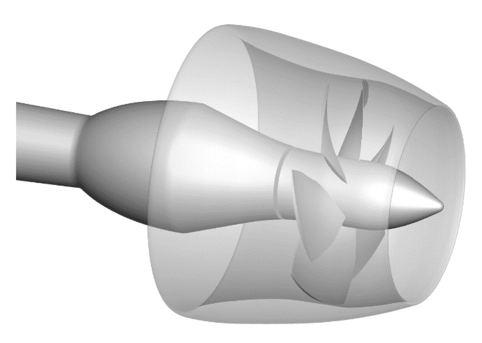
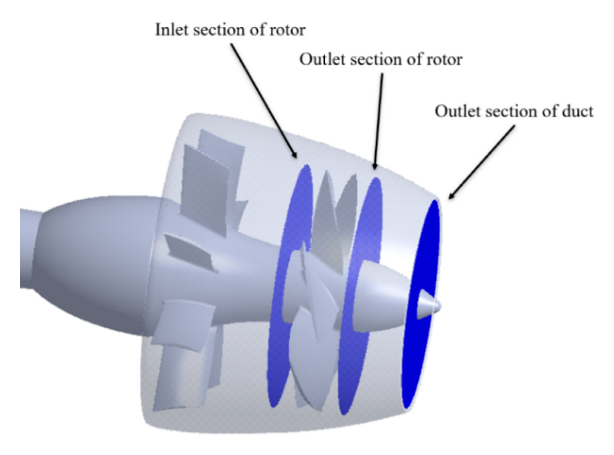
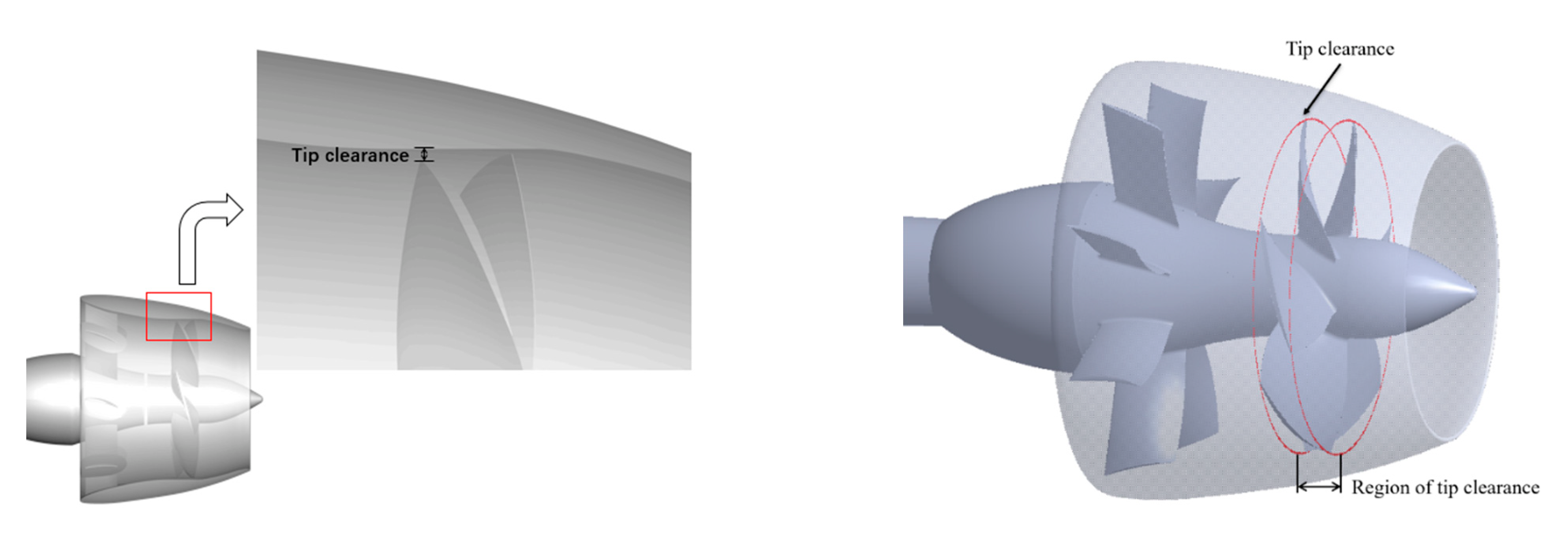
The model of the pumpjet propulsor is shown in Figure 1. It consists of a hub, duct, pre-swirl stator, and rotor. It has 6 rotor blades and 8 pre-swirl stator blades. The diameter of the small-scale rotor is 164.4 mm, while the diameter of the large-scale rotor is 2466 mm. The tip clearance for the small-scale pumpjet propulsor is 2 mm. And the tip clearance for the large-scale pumpjet propulsor is 30 mm.
The right-handed coordinate system is shown in Figure 1. The origin of the coordinate system is at the center of the rotor. The X-axis is along with the hub. The Z-axis is vertical. This coordinate system is used in all parts except those specified.
Considering that the stator has an interaction with the duct and rotor, it is not beneficial to the analysis. Therefore, the numerical simulations without stator are added and compared with the original results to analyze the effects of the stator, rotor, and duct, respectively. The geometry without the stator is shown in Figure 2.
3. Numerical Model
An in-house viscous CFD solver is employed in this study, which solves the continuity and unsteady RANS equations as shown in Equations (1) and (2):
where denotes the component of Reynolds averaged speed. represents the static pressure and ρ means the fluid density. means the direction of the coordinates and is the kinematic viscosity. indicates the Reynolds stress tensor.
In order to make the equations closed, the SST k-ω turbulence model is applied in this research. The SST k-ω turbulence model was put forward by Menter [26]. It is a two-equation eddy-viscosity model and a k-ω formulation is applied in the inner region of the boundary layer. The form of the SST k-ω turbulence model is the same as the standard k-ω turbulence model, but it combines the benefits of the stability of the near-wall k-ω turbulence model and the independence of the external boundary k-ε turbulence model. It can adapt to changes of pressure gradient and separating flow. For the discretization of the governing equations, the finite difference method is used with the second-order difference scheme for the space and time terms. The projection algorithm is applied to solve the velocity-pressure coupling. The wall function model is employed for the simulations of the large-scale pumpjet propulsor to save computing resources. Furthermore, the overset grid method is used to handle the connection of the grids which reduces the difficulty of grid generation, and the rotation of the rotor is also modelled with the dynamic overset grid. In this study, the effect of cavitation is not considered.
3.1. Wall Function Model
The Reynolds number of the large-scale simulation is about 107–108, while the small-scale simulation is about 105–106. They are different by two orders of magnitude. As a result, the near-wall grids of large-scale simulations should be smaller than small-scale simulations. This may make the aspect ratio of grids very large and lead to a great number of grids. To solve this problem, a wall function is needed. It allows the near-wall grids to be arranged in the logarithmic layer (the boundary layer includes the sub-layer, buffer layer, logarithmic layer, and outer region). This will greatly reduce the cost and improves the convergence of the numerical simulations. In the simulations, a multi-layer wall function model [27] is used.
For small-scale pumpjet propulsor simulations, the y+ is less than 1. For large-scale pumpjet propulsor simulations, the wall function is used and the y+ ranges from 10–200. The surface y+ is shown in Figure 3.
3.2. Computational Domain and Boundary Condition
The computational domain in Figure 4 is created for the simulations. It is a cuboid with 6DR (DR denotes the diameter of the rotor) in height and width surrounding the pumpjet propulsor. The two end surfaces of the cuboid are velocity inlet and pressure outlet. The bottom surface is a zero pressure boundary, which means the dynamic pressure is zero and has no effect to the boundary. The other three sides are zero pressure gradient boundaries. The object surface is set as a no-slip wall, where all components of velocity and the normal gradient of static pressure become zero. The center of the rotor is 5DR away from the velocity inlet boundary and is 15DR away from the pressure outlet boundary. The velocity of inflow is given on the velocity inlet.
3.3. Overset Grid Method
The pumpjet propulsor includes a hub, rotor blades, pre-swirl stator blades, and a duct. It is difficult to generate a structured grid wholly. The overset grid method is adapted to this condition by splitting an object into several components and then generating a grid for each component separately.
The overset grid method is aimed at establishing the relationship among each grid and transferring the information of overset grids on the boundary. The overset grid method requires three steps: hole cutting, fringe nodes identification and donor nodes identification. The purpose of hole cutting is to remove the unnecessary nodes (such as the inside of a solid body). The hole mapping method [28] is employed for the hole cutting process and the cut-paste algorithm [29] is applied to generate the overset area. The nodes on the boundary of the overset area are the fringe nodes. The nodes neighbored to the fringe nodes are donor nodes and are searched by the ADT (alternating digital tree) method. The flow information of the fringe nodes is calculated by the flow information of the donor nodes through trilinear interpolation [30]. An optimization is conducted after the donor nodes are searched based on the volume matching or the node distance between fringe nodes and donor nodes to ensure at least two-layer grids for the overset computation. The dynamic overset grid method can realize a real-time arbitrary overset and relative movement between neighboring grids without regenerating the grids.
4. Validation for the Numerical Method
4.1. Verification and Validation for Small-Scale Pumpjet Propulsor
To verify the numerical results, the grid and time step were analyzed. The simulations are performed at J = 0.8. The rotation rate nS is maintained at 22 r/s. The advance ratio of the pumpjet propulsor is set by adjusting the speed of the incoming flow. Table 1 shows the results with different grid numbers and time steps. The associate Courant numbers for the three sets of grids are 0.80, 0.74, and 0.66, respectively. is the total thrust coefficient (including thrust coefficient on the duct, rotor and stator) while is the torque coefficient.
The effect of the grid refinements is evaluated by the grid convergence index (GCI). The calculation is carried out according to Roache [31]:
The fine-grid Richardson error estimator is defined as:
while the medium-grid Richardson error estimator is defined as:
where
In the formulas, is the medium-grid numerical solution and is the fine-grid numerical solution. r21 is the refinement factor between the medium and fine grid. p is the formal order of accuracy of the algorithm which is 2 here.
In addition, a safety factor is incorporated into the estimators and the GCI is defined for fine and medium grids as:
The results for the grid convergence index are given in Table 2. According to the results, the medium grid and medium time step were selected as the uncertainty is small enough.
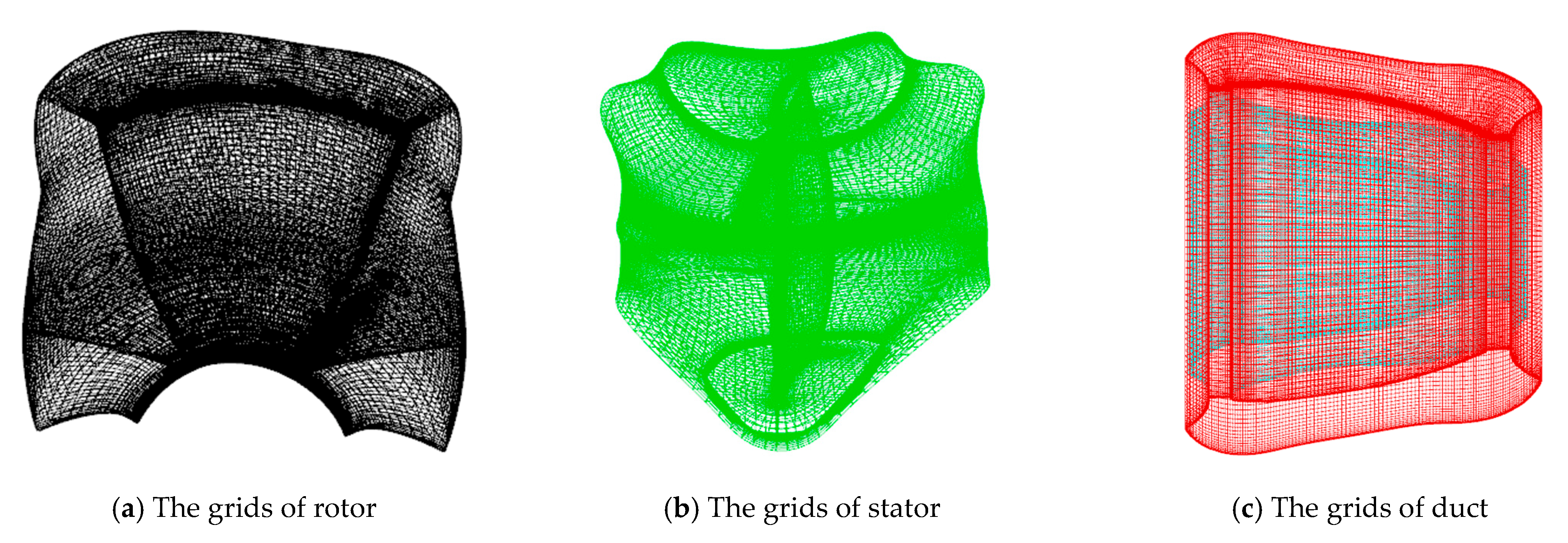
For the selected grid, the surface grid of the rotor is shown in Figure 7a. The number of grids for each rotor blade is about 4.09 × 10⁵. The surface grid of the stator is shown in Figure 7b. The number of grids for each stator blade is about 3.65 × 10⁵. The number of grids for the duct is about 1.51 × 10⁶. The surface grid of the duct is shown in Figure 7c. In the meantime, the corresponding volume grids are shown in Figure 8.
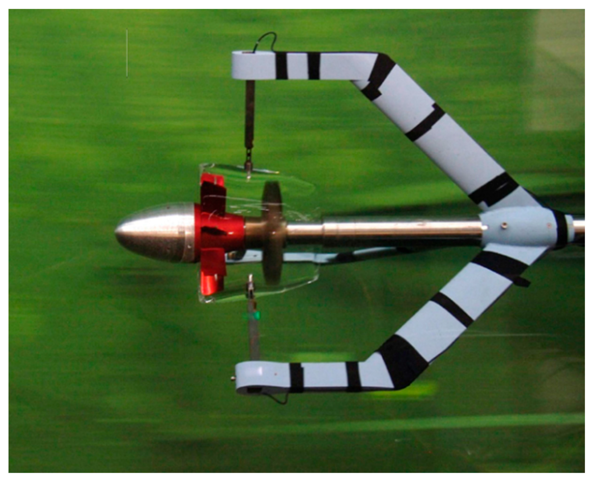
The numerical results of the small-scale pumpjet propulsor are compared with the experimental results (EFD data) from SSSRI (Shanghai Ship and Shipping Research Institute) in Table 3. KTR, KTD, KTS are the thrust coefficient on the rotor, duct and stator, respectively. η0 is the open-water efficiency of the pumpjet propulsor. The experimental setup is shown in Figure 9. Figure 10 is plotted according to the numerical results and experimental results.
The numerical results agree with the experimental data. As can be seen from Figure 10, the total thrust coefficient of the numerical result is slightly smaller than the experimental data, while the torque coefficient is a little larger. Thus, the efficiency is smaller in the results of simulations.
From the numerical results, it can be observed that the efficiency increases first and then decreases with the increasing of the advance ratio. It achieves the maximum value between J = 0.8 and J = 0.9. The thrust and torque coefficients of rotors decrease when the advance ratio increases, and the thrust coefficient of the duct and stators increases in the opposite direction.
4.2. Verification for Large-Scale Pumpjet Propulsor
To ensure the accuracy of the simulations, the grid and time step are verified for the large-scale pumpjet propulsor. The simulations are developed at J = 0.8. The rotation rate for the model test is obviously unreasonable for the large-scale model, so the rotation rate for the large-scale pumpjet propulsor nL is set as 5.68 r/s, according to Froude similarity criterion. To keep the advance ratio the same, the speed of the incoming flow will also be adjusted.
The surface grid of the large-scale pumpjet propulsor is the same as the small-scale pumpjet propulsor and generates the computational grids according to the y+. By refining the nodes as it did for small-scale pumpjet propulsor, three sets of grids are created. The rotor rotates one revolution every 180 time steps in small-scale simulations. This is also the same on the large-scale rotor. Based on this, two more time steps are created to verify this time step. The verification procedure is the same as that in Section 4.1. The results are shown in Table 4. The associate Courant numbers for the three sets of grids are 0.80, 0.74, and 0.66, respectively.
The effect of grid refinements is also evaluated by the grid convergence index (GCI) like the small-scale pumpjet propulsor. The results are given in Table 5. According to the results, the medium grid and medium time step are selected as the uncertainty is small enough.
4.3. Study on the Effect of the Wall Function Model
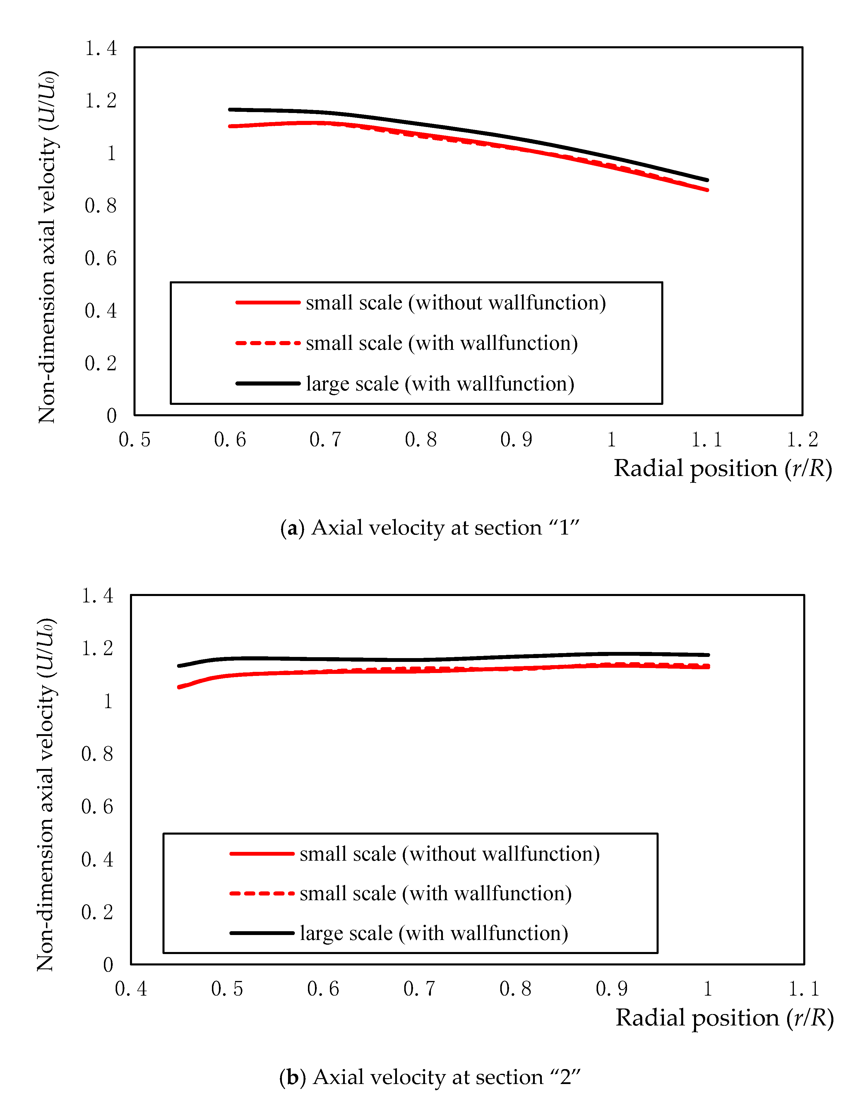
In the simulations of large-scale pumpjet propulsor, the wall function model is introduced to reduce the amount of grid. To study the influence of the wall function model to the results, a simulation was added for the small-scale pumpjet propulsor at J = 0.8 using the wall function model. The axial velocities (U) at the following five sections (shown in Figure 11) are extracted and shown in Figure 12.
According to the comparison, the use of the wall function model leads to no difference and has no effect on the analysis of scale effect.
5. Results and Discussion
For the pumpjet propulsor under these two scales, three advance ratios near the optimal efficiency point are selected for the two scales. Furthermore, the models without a stator are also studied at J = 0.8. According to Froude similarity and the same advance ratio, the rotation rate nS maintains 22 r/s for the small-scale rotor while nL maintains 5.68 r/s for the large-scale rotor. The advance ratio of the pumpjet propulsor is set by adjusting the speed of the incoming flow. For the two scales, J = 0.6, 0.8, and 0.9 are researched. Table 6 presents the comparison of the Reynolds number based on the rotor in the two scales which is defined as:
where b0.75R is the chord length of the rotor blade at r/R = 0.75. The Reynolds number calculated by the chord length of the stator and velocity of the incoming flow is about 105 for the small scale while it is about 6 × 10⁶ for the large scale. Table 7 compares the numerical results for the two scales. In the table, the thrust and torque in the same direction as the rotor are positive. The difference described later is calculated by the formula:
The numerical results under the two scales are obviously different. The efficiency of the large-scale pumpjet propulsor is 8.36% to 9.80% higher than the small-scale pumpjet propulsor. It is because the total thrust is a little larger, while torque is slightly smaller on the large scale. This means it is conservative to predict the pumpjet from a small-scale pumpjet.
From Table 7, it can be judged that the main source of thrust difference between the two scales is the duct. The thrust coefficients on the duct and stator have some difference, but it is smaller than the duct.
In the results, the highest efficiency appears at J = 0.8 in both scales. As a result, more observations at J = 0.8 were made to find out the difference. To understand the different distribution of different components between the two scales, the coefficients were divided into pressure component and friction component. The specific results are listed in Table 8.
From Table 8, the friction component varies a lot between the two scales. This is mainly affected by different Reynolds numbers between two scales and leads to the difference of viscosity. There are also some differences in the pressure component. This is caused by the interaction of stator, rotor, and duct. The main difference is observed between the duct and rotor. These differences are analyzed in the following sections. All the analyses are based on the results that the advance ratio is 0.8.
5.1. Difference About the Stator
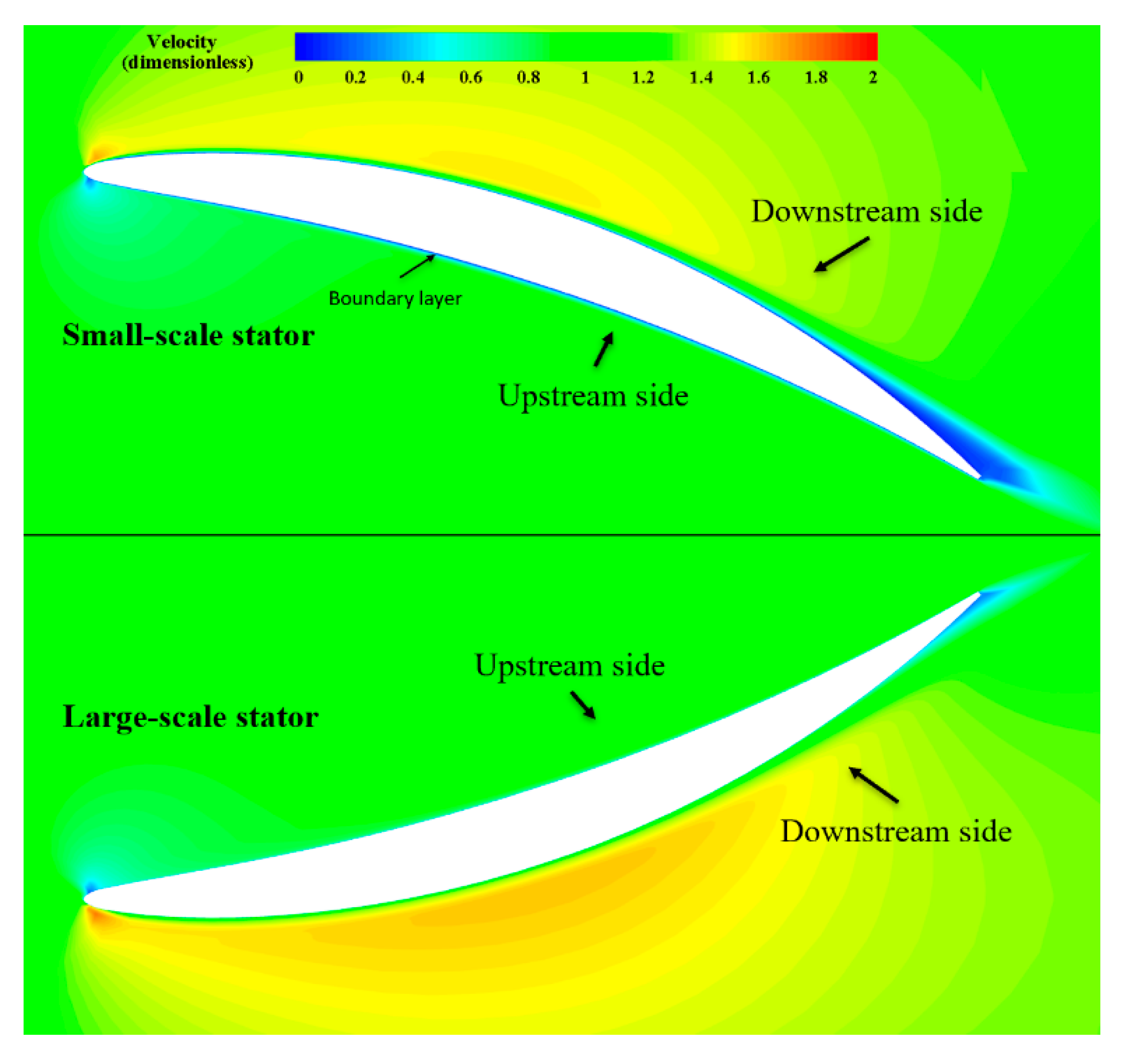
According to the relative position from the incoming flow, the stator blade is divided into the upstream side and the downstream side. Figure 13 shows the flow field of the two scales at the radial position of r/R = 0.75 near the stator. R represents the radius of rotor and r denotes the radial position. There are clear differences in the development of flow field. In the figure, the blue color block represents the low speed area. The boundary layer is obvious only near the small-scale stator. As for the downstream side, flow separation is more likely to occur on the tail of the small-scale stator because of the lower Reynold numbers. The fluid close to the downstream side will flow more and more slowly under the action of wall friction. In this case, flow separation will eventually occur. But flow separation is more likely to occur at small scales which results in the low-speed area near the tail.
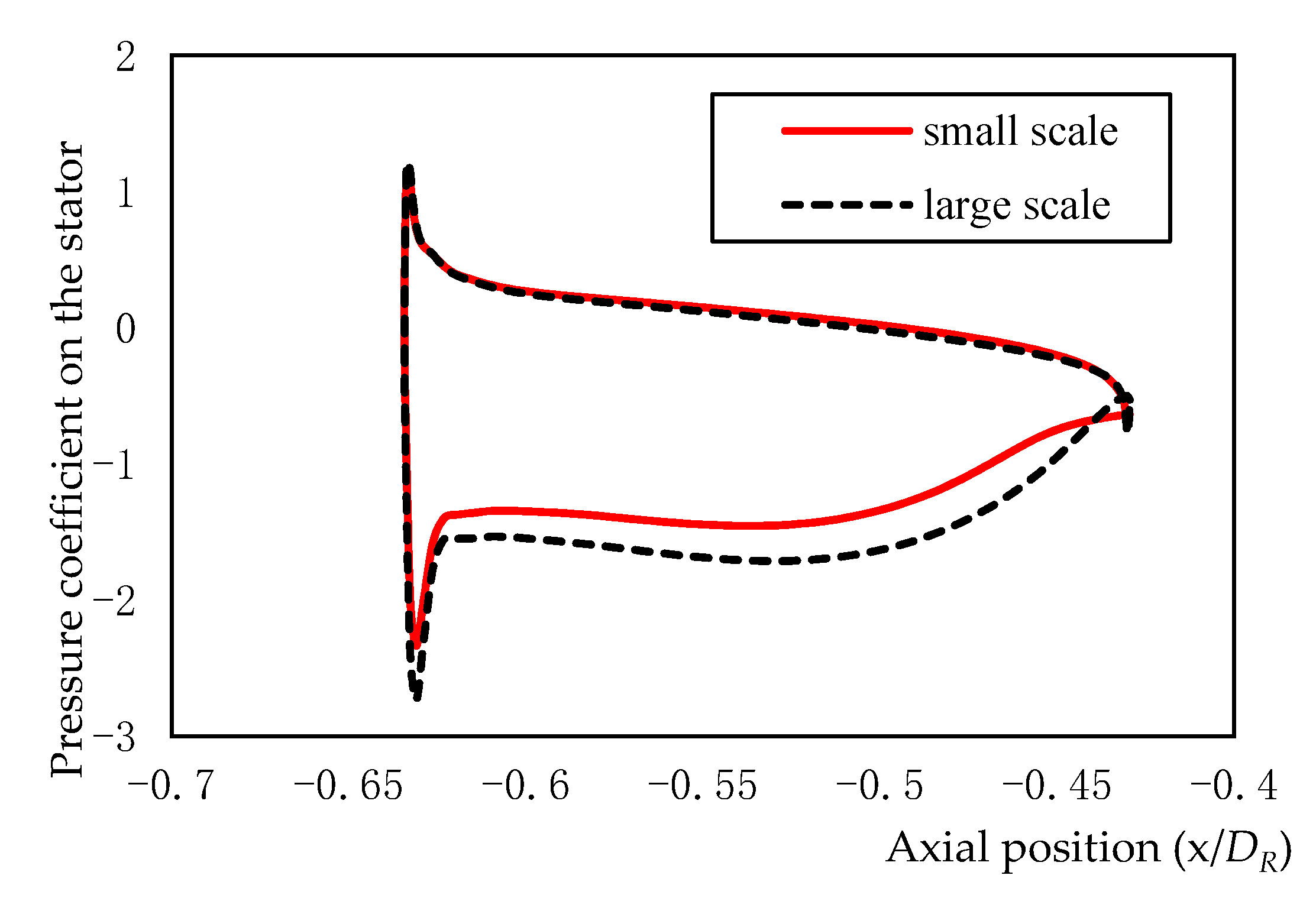
Figure 14 shows the pressure coefficient around the surface at the radial position of r/R = 0.75. The pressure distribution is related to the flow field. Because of the similar flow field near the upstream side, the pressure distribution on the upstream side is almost the same for the two-scale pumpjet propulsor. As for the downstream side, the difference in flow development leads to obvious differences in pressure distribution at the two scales. Furthermore, the pressure distribution at the flow separation area is almost the same as that at the beginning point of flow separation. Thus, the relationship between the value of the pressure on the tail between the two scales has changed. These result in the difference of the thrust coefficient on the stator.
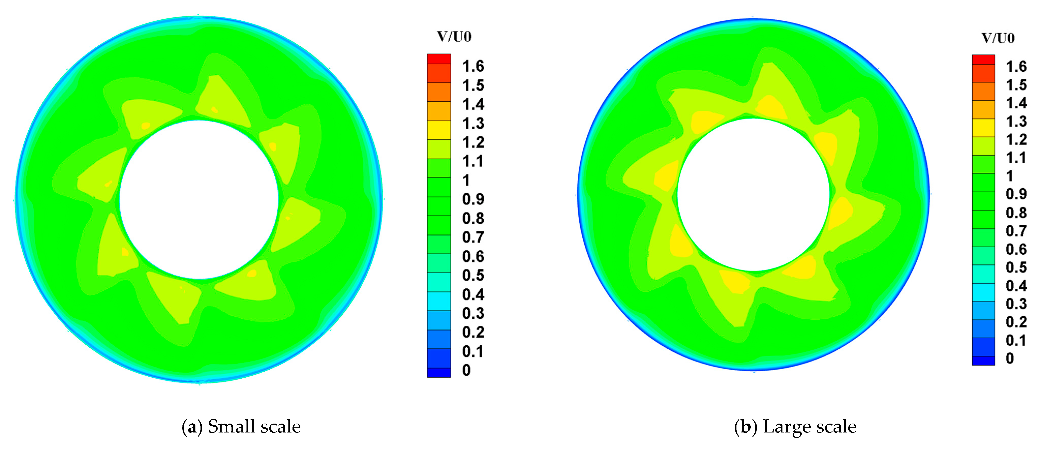
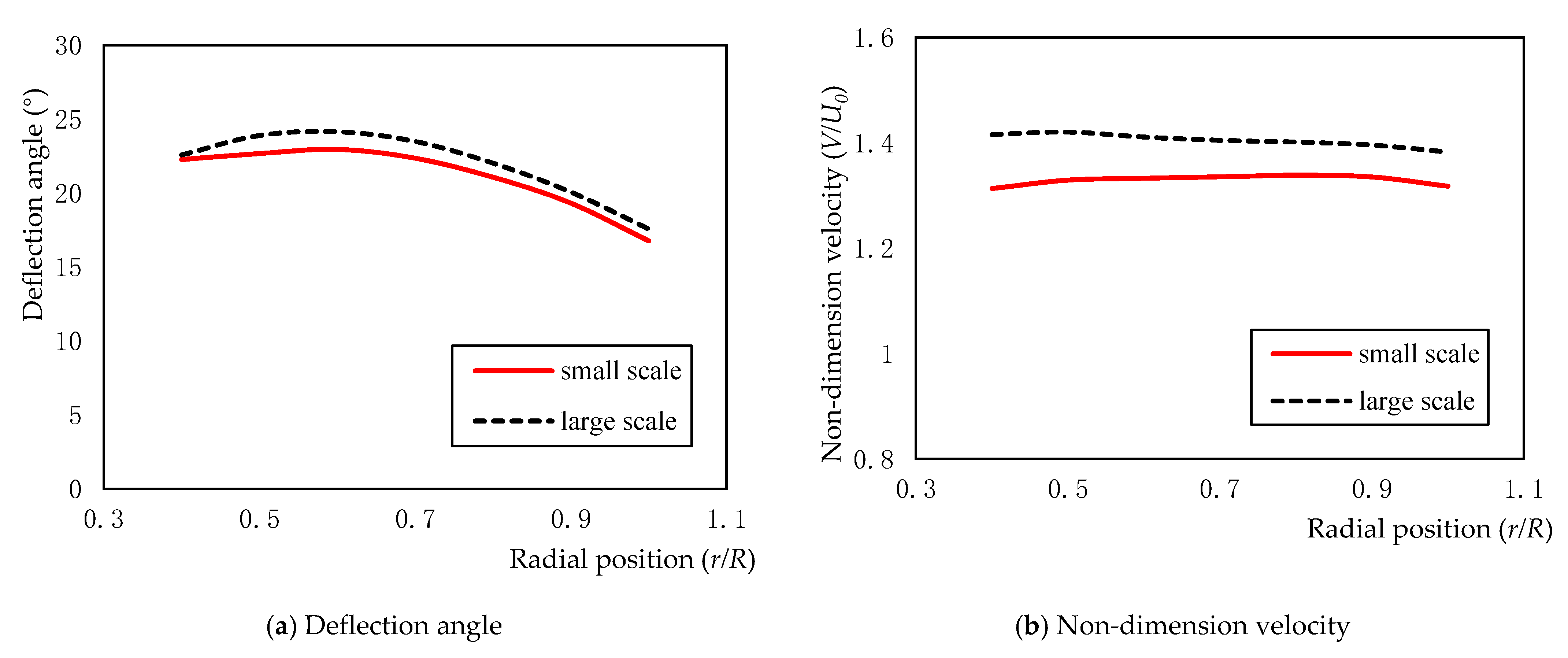
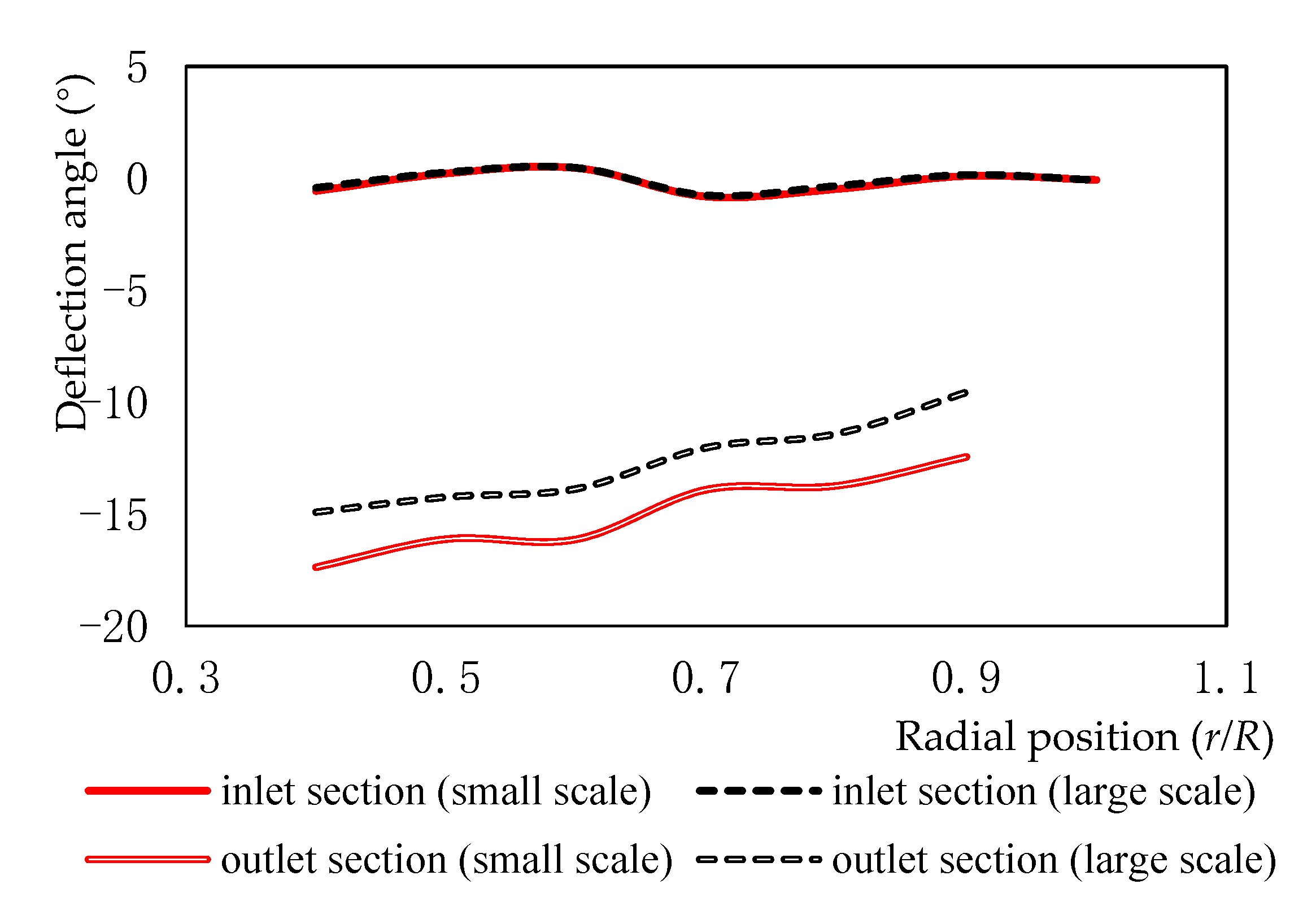
Due to the acceleration effect of the duct and the suction effect of the rotor, the incoming flow will be accelerated and deflected when approaching the inlet section of the stator. After being deflected by the stator, there is a large deflection angle for the flow at the outlet section of the stator which is different for the two scales. And the velocity near the large-scale stator is always higher than the small-scale stator which is caused by the viscosity of the stator surface. As a result, the development of the flow after the stator can also be impacted. To show this more clearly, the velocity and deflection angle are observed in three sections. Figure 15 shows the selected three sections. The deflection angle is defined as the angle between the resultant velocity and the axial direction (shown in Figure 16). Figure 17, Figure 18 and Figure 19 show the velocity field. To quantify the data in the graph, the average data at each radius is taken to get Figure 20, Figure 21 and Figure 22. It is observed that the flow within the duct always has some differences between the two scales. It is the viscosity on the stator and hub that leads to the difference. After the flow passing through the stator, the flow will have an impact on the duct and rotor making the differences between the two scales which is analyzed in Section 5.2 and Section 5.3.
For the pumpjet propulsor, the torque on the duct is very small, while the torque on the stator and rotor is the opposite. When the design is reasonable, the entire device can achieve torque balance. To verify the torque balance of the device, Table 9 presents the torque coefficient of the rotor and the stator for the two scales. For the small-scale pumpjet propulsor, the difference of the torque coefficient between the rotor and the stator is smaller than the large-scale pumpjet propulsor. This means that the scale will affect the torque balance design of the pumpjet propulsor. For the pumpjet propulsor in this study, the torque on the stator and rotor of the small-scale pumpjet propulsor is relatively close, while the torque on the rotor and stator of the large-scale pumpjet propulsor is not.
5.2. Difference About the Rotor
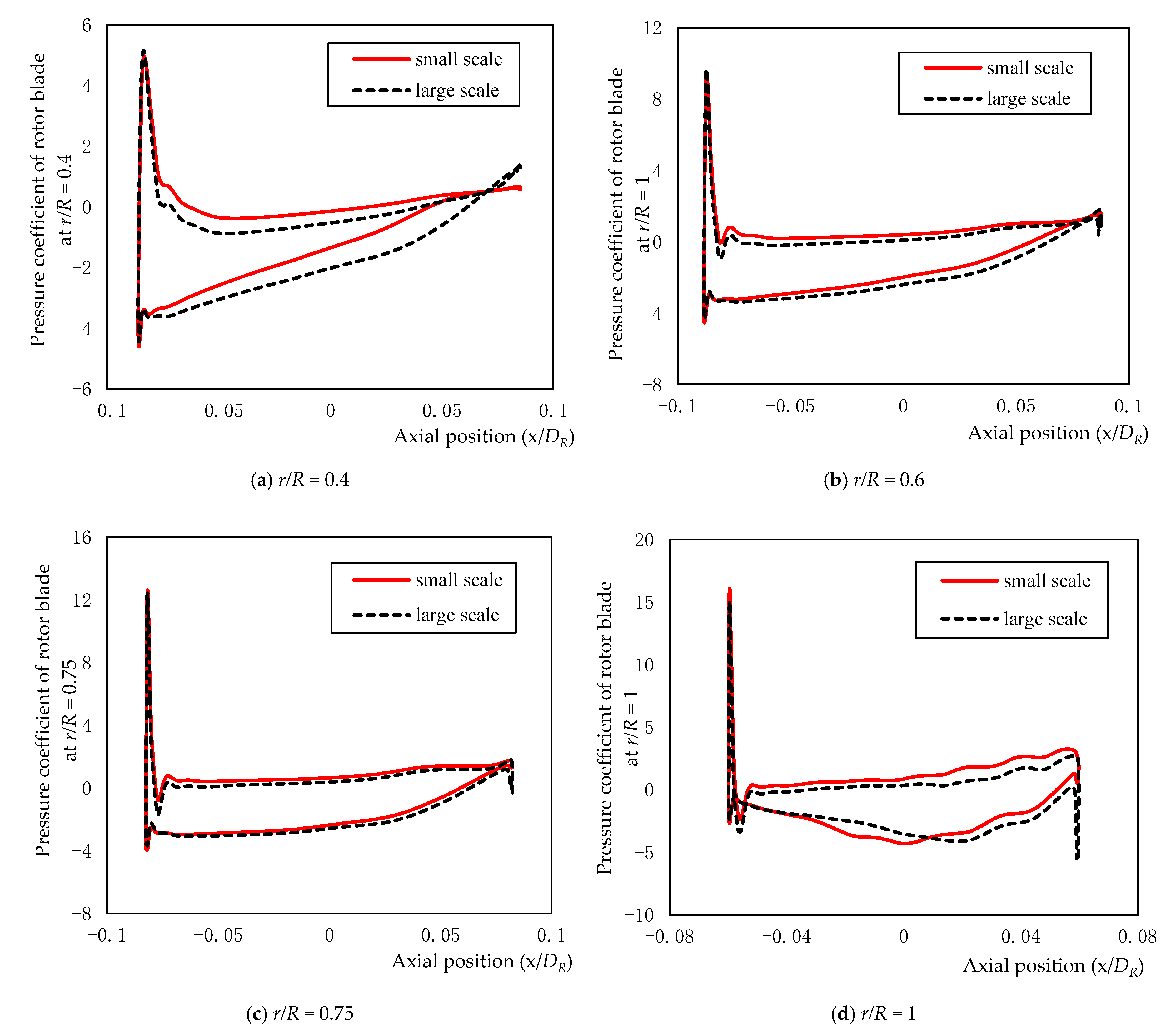
Figure 23 shows the pressure coefficient (defined as P/0.5ρSV²) at the radial position of r/R = 0.4, 0.6, 0.75, and 1. The leading edge is located at the minimum axial position, while the trailing edge is located at the maximum axial position.
The pressure coefficient on the leading edge is almost the same between the two scales. With the development of the flow, different pressure distribution appears on the blade. And there are obvious differences on the trailing edge, especially at large radius.
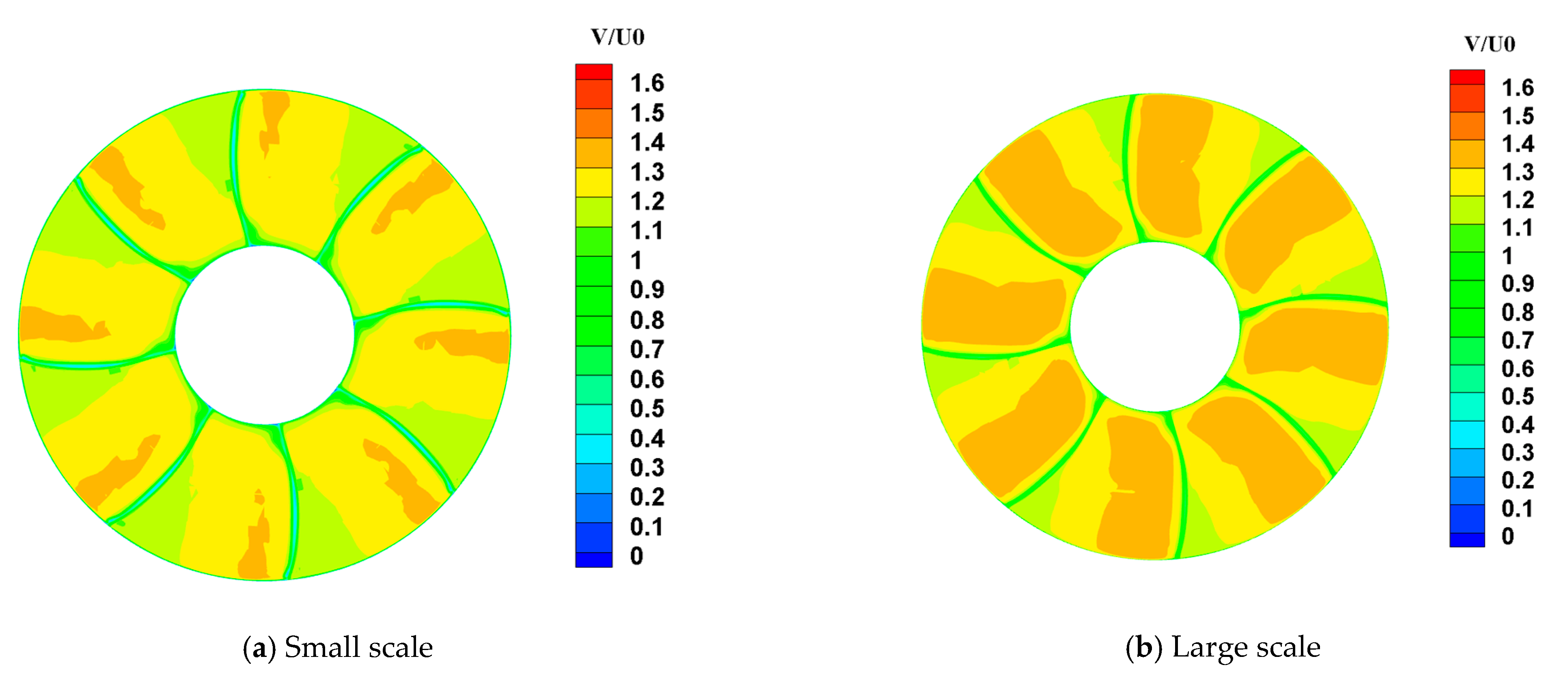
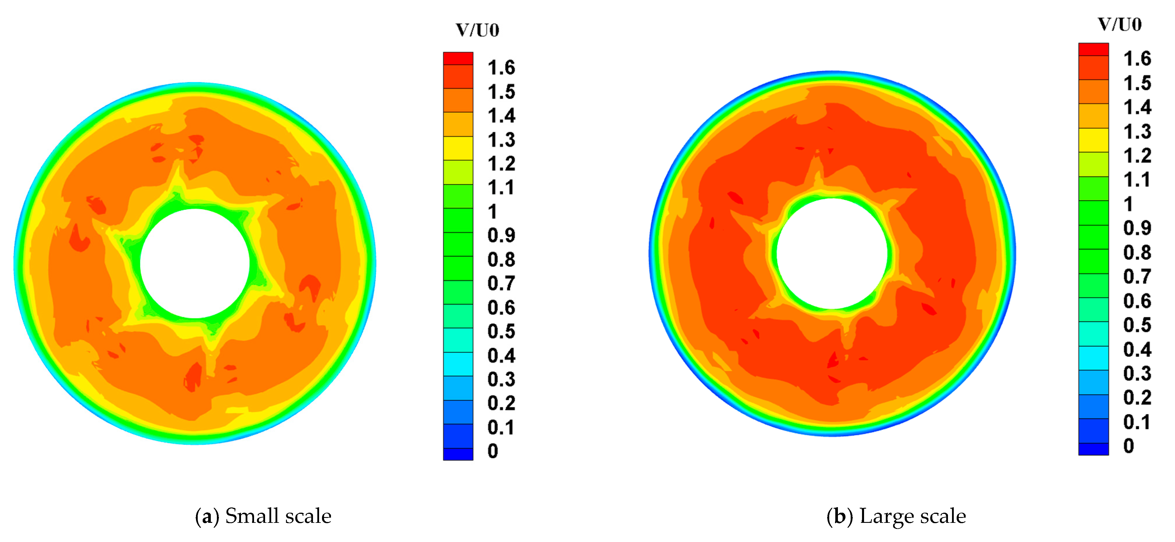
The stator will influence the velocity field and deflection angle, then influence the flow field near the rotor. Thus, the velocity and deflection angle on the inlet and outlet section of the rotor (sketch of the sections are shown in Figure 24) are observed. Figure 25 and Figure 26 present the comparison of velocity at the inlet and outlet sections of the rotor. To quantify the data in the graph, the average velocity and deflection angle at each radius is taken to get Figure 27 and Figure 28.
The inflow is accelerated and deflected by the rotor. The attack angle of a blade element is associate with the deflection angle of flow and the installation angle of the blade element. The installation angle of the same blade element is the same between the rotors of two scales. But the deflection angle is different between the two scales. The deflection of the stator to the incoming flow is different at different scales which leads to different effective attack angles of blade elements at the same position. In addition, the non-dimension velocity of the large-scale pumpjet propulsor is greater at the inlet and outlet sections of the rotor according to Figure 27 and Figure 28. This is equivalent to the large-scale rotor working at a higher effective advance ratio. As a result, the pressure distribution on the blade surface will be different which shows the difference caused by the stator.
To distinguish the effect of different parts, simulations for the two pumpjet propulsors without the stator are added. For the simulations without the stator, the deflection angle of the incoming flow for the rotor will be zero, and there is no friction loss on the stator. However, the friction on the duct will also exist. Figure 29 and Figure 30 present the deflection angle and velocity on the two sides of the rotor. Compared to Figure 27 and Figure 28, the deflection angles in front of the rotor are almost the same. The velocity around the rotor will be lower without the stator and the difference between the two scales is smaller than that with stator.
Figure 31 shows the axial force coefficient (defined as F/0.5ρSV²) at the different radius of the rotor. The difference on the rotor of two scales with and without the stator varies a lot when r/R < 0.7, which means the stator has made a big impact on the scale effect of the rotor.
When there is no stator, the difference is caused by the friction on the duct which influences the incoming flow (shown in Figure 30) when r/R < 0.9. As for r/R > 0.9, the trend of the curves has changed and it is the tip clearance that mainly leads to the difference. The region of tip clearance ranges from x/DR = −0.06 to 0.06 and it is shown in Figure 32. The size of the tip clearance between the two scales is different according to the scale ratio which can affect the flow field. Thus, the average flow velocity in the tip clearance is extracted. Figure 33a shows the average non-dimension axial velocity in the tip clearance at different axial positions while Figure 33b shows the average non-dimension circumferential velocity. According to Figure 33, the velocity in the tip clearance between the two scales has an obvious difference. For both two scales, there will be an obvious reverse velocity near the trailing edge, which means it will appear to backflow in the tip clearance. However, for the large-scale tip clearance, only a region much smaller than the small-scale tip clearance near the trailing edge appears to backflow. The important difference arises from this.
Except for the axial force coefficient, the circumferential force coefficient also has a significant difference. Figure 34 shows the average circumferential force coefficient of the rotor at different radial positions. If one only focuses on the relationship between absolute values, the distribution of the circumferential force coefficient is very similar to the distribution of the axial force coefficient.
5.3. Difference About the Duct
To distinguish the effect of the stator and rotor on the duct, the simulation results without the stator are also presented for comparison. Figure 35 presents the axial force coefficient distribution on the exterior and interior sides of the duct. Furthermore, the results of the simulations without the stator are shown in Figure 36.
The thrust coefficient on the exterior side of the duct is almost the same in the front and middle according to Figure 35a, while there is a difference on the tail of duct. The difference mainly comes from the flow separation and the wake. According to Figure 37, it can be observed that flow separation occurs on the exterior side of the tail of the duct. The upper part of the figure shows the flow field near the smaller-scale duct, and the lower part shows the flow field near the larger one. With the development of the flow on the surface of the duct, flow separation is more likely to occur on the exterior side of the small-scale duct because of the lower Reynold numbers. This results in the difference at the exterior side of the duct in Figure 35a. Bhattacharyya [23] also found the same situation on the exterior side of the duct when researching a ducted propeller. In addition, according to Figure 35a and Figure 36a, it can be concluded that the stator also has a little influence on the exterior side of duct. The slight difference is caused by the flow field at the inlet and outlet section of the duct which changes with the effect of the stator.
When compared with the interior side of the duct, the difference on the exterior side of the duct is more obvious and it is the main source of difference on the duct according to Figure 35. At the axial position ranging from −0.6~−0.1 DR, there is a significant difference between the two scales. In the simulation without a stator, the difference almost disappears according to the results in Figure 36b. Thus, we concluded that it is due to the difference of the stator. According to Section 5.1, the flow development on the downstream side of the stator is different in two scales, which leads to the different flow states at the intersection of the stator and duct. This is the main source of the difference at the interior side of the duct at the axial position ranging from −0.6–−0.1 DR. At the axial position ranging from 0.1–0.35 DR, the tail of the duct contracts inward and blocks the fluid from passing through. The contracted part of the duct is impacted by the fluid and is subjected to a backward force. The flow state near the wall will be influenced by the rotor and the tip clearance. This leads to the difference at the interior side of the duct at the axial position ranging from 0.1–0.35 DR. At the axial position ranging from 0.35–0.4 DR, the trend of the axial force coefficient has changed from before. It is because the tail of the duct blocks the development of outward flow and forms a high-speed region at the tail. This can be observed in Figure 37. The difference relates to the flow field at the outlet section of the duct. The comparison of the velocity at the outlet section of the duct (the position of the section is shown in Figure 24) is given in Figure 38. The flow field near the surface of duct which is affected by the stator and rotor has a large difference in the deflection angle between the two scales.
6. Conclusions
A numerical study of a pumpjet propulsor using an in-house viscous CFD solver is presented. The numerical results calculated by the solver are compared with the experimental results and they are in good agreement. It indicates that the solver is reliable.
The performances of the stator, rotor and duct have certain differences under different scales. The analysis is performed near optimal point. Because of the different Reynolds numbers, the friction component in each part is about 40% smaller for the large-scale pumpjet propulsor. It obviously influences the torque coefficient. The torque coefficient of the large-scale rotor is smaller than the small-scale one, in which the friction component accounts for 63% of the reduction. Compared with the friction component, the absolute value of the pressure component is much greater and distributes more to the difference of the total thrust coefficient.
As for the stator, the development of flow field and pressure distribution on the upstream side between the two scales are almost the same. The difference is mainly observed on the downstream side. It is the different flow field that leads to the different pressure distribution. Furthermore, when the design is reasonable, the stator can balance the torque of the rotor to a certain extent, so as to achieve torque balance. But the torque balance will also be influenced by scale.
As for the rotor, the thrust and torque are influenced by the stator and the tip clearance. Because of the different flow fields after the stator between different scales, the non-dimension velocity and deflection angle are different for the rotor. This will directly affect the performance of the rotor. Furthermore, the velocity of flow in the tip clearance varies a lot between different scales and has an influence on the rotor, especially at the larger radial position. The influence of tip clearance gradually decreases when it is far away from the tip clearance.
As for the duct, the small-scale duct presents a greater negative contribution to the total thrust coefficient than the large-scale duct. On the exterior side, the flow separation is more likely to appear for a small scale and leads to the difference at the tail of the duct. But the difference of flow separation is not obvious and the region is small so that it contributes little to the thrust coefficient. As for the interior side of the duct, the difference is more obvious than the exterior side. The former half of the interior side is influenced by the viscosity of the stator surface, while the latter half is influenced by the flow after the rotor which involved the stator and rotor.
In summary, the duct and stator have a negative contribution to the total thrust and the rotor has a positive contribution to the total thrust. Under these two scales, the thrust coefficient on the duct is smaller and the thrust coefficient on stator is greater for the large-scale pumpjet propulsor. As for the rotor, the thrust coefficient is smaller for the large-scale rotor. As a result, the total thrust coefficient is larger on the large-scale pumpjet propulsor. The torque coefficient is smaller on the large-scale rotor. Thus, the efficiency of the large-scale pumpjet propulsor is about 8–10% higher than the small-scale one. Therefore, the impact of scale cannot be ignored when predicting the performance of pumpjet propulsors.
Author Contributions
Investigation, writing–original draft, writing–review and editing, data curation, visualization, J.Y.; project administration, methodology, resources, funding acquisition, supervision, D.F.; writing–review and editing, supervision, L.L.; supervision, resources, X.W.; supervision, resources, C.Y. All authors have read and agreed to the published version of the manuscript.
Funding
This research was funded by the China National Science Foundation YEQISUN Joint Funds grant number U2141228.
Institutional Review Board Statement
Not applicable.
Informed Consent Statement
Not applicable.
Data Availability Statement
Not applicable.
Acknowledgments
We appreciate the help of the Marine Design and Research Institute of China for providing the model and the Shanghai Ship and Shipping Research Institute for providing the model test data.
Conflicts of Interest
The authors declare no conflict of interest.
Nomenclature
| DR | m | Diameter of rotor |
| r | m | Distance from any point to the X-axis |
| R | m | Radius of rotor |
| b0.75 | m | Chord length of the rotor blade at r/R = 0.75 |
| U0 | m/s | Velocity of inflow |
| V | m/s | Velocity at any point |
| n | r/s | Rotational speed of rotor (subscript “S” means small scale and subscript “L” means large scale) |
| J | / | Advance coefficient, |
| Re0.75 | / | Reynolds number based on blade chord length at 0.75R and velocity of inflow, |
| ν | kg/m³ | Density of water |
| KTR | / | Thrust coefficient of rotor |
| KTD | / | Thrust coefficient of duct |
| KTS | / | Thrust coefficient of stator |
| KT | / | Total thrust coefficient, including thrust coefficient of rotor (KTR), duct (KTD), stator (KTS) |
| KQ | / | Torque coefficient of rotor, |
| KQS | / | Torque coefficient of stator |
| η0 | / | Efficiency of pumpjet propulsor, |
References
- Gong, J.; Guo, C.-Y.; Zhao, D.-G.; Wu, T.-C.; Song, K.-W. A comparative DES study of wake vortex evolution for ducted and non-ducted propellers. Ocean Eng. 2018, 160, 78–93. [Google Scholar] [CrossRef]
- Zhang, Q.; Jaiman, R.K. Numerical analysis on the wake dynamics of a ducted propeller. Ocean Eng. 2018, 171, 202–224. [Google Scholar] [CrossRef]
- Gaggero, S. Numerical design of a RIM-driven thruster using a RANS-based optimization approach. Appl. Ocean Res. 2019, 94, 101941. [Google Scholar] [CrossRef]
- Liu, B.; Vanierschot, M. Numerical Study of the Hydrodynamic Characteristics Comparison between a Ducted Propeller and a Rim-Driven Thruster. Appl. Sci. 2021, 11, 4919. [Google Scholar] [CrossRef]
- ITTC. 1978 ITTC Performance Prediction Method. In ITTC-Recommended Procedures and Guidelines; ITTC: Zürich, Switzerland, 2017. [Google Scholar]
- Yao, H.; Zhang, H. Numerical simulation of boundary-layer transition flow of a model propeller and the full-scale propeller for studying scale effects. J. Mar. Sci. Technol. 2018, 23, 1004–1018. [Google Scholar] [CrossRef]
- Dong, X.-Q.; Li, W.; Yang, C.-J.; Noblesse, F. RANSE-based simulation and analysis of scale effects on open-water performance of the PPTC-II benchmark propeller. J. Ocean Eng. Sci. 2018, 3, 186–204. [Google Scholar] [CrossRef]
- Lungu, A. Scale Effects on a Tip Rake Propeller Working in Open Water. J. Mar. Sci. Eng. 2019, 7, 404. [Google Scholar] [CrossRef] [Green Version]
- Yang, Q.; Wang, Y.; Zhang, Z. Scale effects on propeller cavitating hydrodynamic and hydroacoustic performances with non-uniform inflow. Chin. J. Mech. Eng. 2013, 26, 414–426. [Google Scholar] [CrossRef]
- Sanchez-Caja, A.; González-Adalid, J.; Pérez-Sobrino, M.; Sipilä, T. Scale effects on tip loaded propeller performance using a RANSE solver. Ocean Eng. 2014, 88, 607–617. [Google Scholar] [CrossRef]
- Soydan, A.; Bal, S. An investigation of scale effects on marine propeller under cavitating and non-cavitating conditions. Ship Technol. Res. 2021, 68, 166–178. [Google Scholar] [CrossRef]
- Castro, A.M.; Carrica, P.M.; Stern, F. Full scale self-propulsion computations using discretized propeller for the KRISO container ship KCS. Comput. Fluids 2011, 51, 35–47. [Google Scholar] [CrossRef]
- Sun, S.; Wang, C.; Guo, C.; Zhang, Y.; Sun, C.; Liu, P. Numerical study of scale effect on the wake dynamics of a propeller. Ocean Eng. 2019, 196, 106810. [Google Scholar] [CrossRef]
- Gao, H.; Lin, W.; Du, Z. Numerical flow and performance analysis of a water-jet axial flow pump. Ocean Eng. 2008, 35, 1604–1614. [Google Scholar] [CrossRef]
- Lu, L.; Pan, G.; Sahoo, P.K. CFD prediction and simulation of a pumpjet propulsor. Int. J. Nav. Archit. Ocean. Eng. 2016, 8, 110–116. [Google Scholar] [CrossRef] [Green Version]
- Qin, D.; Pan, G.; Huang, Q.; Zhang, Z.; Ke, J. Numerical Investigation of Different Tip Clearances Effect on the Hydrodynamic Performance of Pumpjet Propulsor. Int. J. Comput. Methods 2018, 15, 1850037. [Google Scholar] [CrossRef] [Green Version]
- Pan, G.; Lu, L.; Sahoo, P.K. Numerical simulation of unsteady cavitating flows of pumpjet propulsor. Ships Offshore Struct. 2015, 11, 64–74. [Google Scholar] [CrossRef]
- Ahn, S.J.; Kwon, O.J. Numerical investigation of a pump-jet with ring rotor using an unstructured mesh technique. J. Mech. Sci. Technol. 2015, 29, 2897–2904. [Google Scholar] [CrossRef]
- Li, H.; Pan, G.; Huang, Q. Transient analysis of the fluid flow on a pumpjet propulsor. Ocean Eng. 2019, 191, 106520. [Google Scholar] [CrossRef]
- Suryanarayana, C.; Satyanarayana, B.; Ramji, K.; Saiju, A. Experimental evaluation of pumpjet propulsor for an axisymmetric body in wind tunnel. Int. J. Nav. Archit. Ocean. Eng. 2010, 2, 24–33. [Google Scholar] [CrossRef] [Green Version]
- Shirazi, A.T.; Nazari, M.R.; Manshadi, M.D. Numerical and experimental investigation of the fluid flow on a full-scale pump jet thruster. Ocean Eng. 2019, 182, 527–539. [Google Scholar] [CrossRef]
- Bhattacharyya, A.; Krasilnikov, V.; Steen, S. Scale effects on open water characteristics of a controllable pitch propeller working within different duct designs. Ocean Eng. 2016, 112, 226–242. [Google Scholar] [CrossRef]
- Bhattacharyya, A.; Krasilnikov, V.; Steen, S. A CFD-based scaling approach for ducted propellers. Ocean Eng. 2016, 123, 116–130. [Google Scholar] [CrossRef]
- Feng, D.; Yu, J.; He, R.; Zhang, Z.; Wang, X. Improved body force propulsion model for ship propeller simulation. Appl. Ocean Res. 2020, 104, 102328. [Google Scholar] [CrossRef]
- Liu, L.; Chen, M.; Yu, J.; Zhang, Z.; Wang, X. Full-scale simulation of self-propulsion for a free-running submarine. Phys. Fluids 2021, 33, 047103. [Google Scholar] [CrossRef]
- Menter, F.R. Two-equation eddy-viscosity turbulence models for engineering applications. AIAA J. 1994, 32, 1598–1605. [Google Scholar] [CrossRef] [Green Version]
- Bhushan, S.; Xing, T.; Carrica, P.; Stern, F. Model- and Full-Scale URANS Simulations of Athena Resistance, Powering, Seakeeping, and 5415 Maneuvering. J. Ship Res. 2009, 53, 179–198. [Google Scholar] [CrossRef]
- Chiu, I.; Meakin, R.L. On Automating Domain Connectivity for Overset Grids. In Proceedings of the 33rd Aerospace Sciences Meeting and Exhibit, NASA Ames Research Center Advanced Design Cycle Branch, Los Altos, CA, USA, 9–12 January 1995. [Google Scholar]
- Cho, K.W.; Kwon, J.H.; Lee, S. Development of a Fully Systemized Chimera Methodology for Steady/Unsteady Problems. J. Aircr. 1999, 36, 973–980. [Google Scholar] [CrossRef]
- Bonet, J.; Peraire, J. An alternating digital tree (ADT) algorithm for 3D geometric searching and intersection problems. Int. J. Numer. Methods Eng. 1991, 31, 1–17. [Google Scholar] [CrossRef]
- Roache, P.J. Quantification of uncertainty in computational fluid dynamics. Annu. Rev. Fluid Mech. 1997, 29, 123–160. [Google Scholar] [CrossRef] [Green Version]
Figure 1.
The model of the pumpjet propulsor.

Figure 2.
The geometry without stator.

Figure 3.
Surface y+ of the two scale simulations.

Figure 4.
Boundary conditions of the computational domain.

Figure 5.
Overset process between rotor and hub.

Figure 6.
Overset process between stator, duct and hub.

Figure 7.
Surface grids of the rotor, stator and duct.

Figure 8.
Volume grids of the rotor, stator and duct.

Figure 9.
Experimental device.

Figure 10.
Results comparison between CFD and EFD.

Figure 11.
The selected five sections.

Figure 12.
Axial velocities at the five sections.


Figure 13.
The velocity distribution around the stator at r/R = 0.75.

Figure 14.
The pressure distribution on the stator at r/R = 0.75.

Figure 15.
Sketch of the three sections near the stator.

Figure 16.
Sketch of the circumferential velocity.

Figure 17.
Velocity comparison at the inlet section of the stator.

Figure 18.
Velocity comparison at the outlet section of the stator.

Figure 19.
Velocity comparison at the inlet section of the rotor.

Figure 20.
Comparison at the inlet section of the stator.

Figure 21.
Comparison at the outlet section of the stator.

Figure 22.
Comparison at the inlet section of the rotor.

Figure 23.
Pressure coefficient on the surface of the rotor at different radius.

Figure 24.
Sketch of the three sections near the rotor.

Figure 25.
Comparison of velocity at the inlet section of the rotor.

Figure 26.
Comparison of velocity at the outlet section of the rotor.

Figure 27.
Deflection angle on two sides of the rotor.

Figure 28.
Velocity on two sides of the rotor.

Figure 29.
Deflection angle on two sides of the rotor (without stator).

Figure 30.
Velocity on two sides of the rotor (without stator).

Figure 31.
Distribution of the axial force coefficient on the rotor.

Figure 32.
Sketch of the tip clearance region.

Figure 33.
Non-dimension velocity at tip clearance. (a) Non-dimension axial velocity at tip clearance. (b) Non-dimension circumferential velocity at tip clearance.
Figure 33.
Non-dimension velocity at tip clearance. (a) Non-dimension axial velocity at tip clearance. (b) Non-dimension circumferential velocity at tip clearance.

Figure 34.
Average torque coefficient distribution of the rotor. (a) Average torque coefficient distribution of the rotor. (b) Average torque coefficient distribution of the rotor (without stator).
Figure 34.
Average torque coefficient distribution of the rotor. (a) Average torque coefficient distribution of the rotor. (b) Average torque coefficient distribution of the rotor (without stator).

Figure 35.
Distribution of the axial force coefficient on the duct.

Figure 36.
Distribution of the axial force coefficient on the duct (without stator).

Figure 37.
Comparison of flow fields at two scales.

Figure 38.
Comparison of the velocity at the outlet of the duct.


Table 1.
Sensitivity analysis for the small-scale pumpjet propulsor.
| Grids Number | KT | 10KQ | Time Step/s | KT | 10KQ |
|---|---|---|---|---|---|
| 12.58 × 10⁶ | 0.3960 | 0.9796 | 1.785 × 10⁻⁴ | 0.4025 | 0.9870 |
| 9.97 × 10⁶ | 0.4015 | 0.9866 | 2.525 × 10⁻⁴ | 0.4015 | 0.9866 |
| 7.15 × 10⁶ | 0.4024 | 0.9879 | 3.571 × 10⁻⁴ | 0.3833 | 0.9662 |
Table 2.
Calculation for grid convergence index of the small-scale pumpjet propulsor.
| KT | 10KQ | |
|---|---|---|
| 0.4024 | 0.9879 | |
| 0.4015 | 0.9866 | |
| 0.396 | 0.9796 | |
| 1.0806 | 1.0806 | |
| 1.1172 | 1.1172 | |
| −0.0055 | −0.007 | |
| −0.0009 | −0.0013 | |
| p | 2 | 2 |
| 0.0054 | 0.0078 | |
| 0.0063 | 0.0091 | |
| 0.0067 (1.67%) | 0.0097 (0.98%) | |
| 0.0078 (1.95%) | 0.0113 (1.15%) |
Table 3.
Comparison of CFD and EFD results.
| J | KTR | KTD + KTS | 10KQ | η0 | |
|---|---|---|---|---|---|
| 0.6 | EFD | 0.6566 | −0.1321 | 1.0201 | 0.4910 |
| CFD | 0.6355 | −0.1270 | 1.0416 | 0.4662 | |
| Difference | −2.50% | −3.86% | 2.11% | −5.05% | |
| 0.8 | EFD | 0.6081 | −0.1904 | 0.9650 | 0.5511 |
| CFD | 0.5812 | −0.1797 | 0.9866 | 0.5181 | |
| Difference | −4.42% | −5.62% | 2.24% | −5.98% | |
| 0.9 | EFD | 0.5771 | −0.2161 | 0.9296 | 0.5563 |
| CFD | 0.5400 | −0.2026 | 0.9376 | 0.5155 | |
| Difference | −6.43% | −6.25% | 0.86% | −7.34% | |
| 1 | EFD | 0.5415 | −0.2399 | 0.8889 | 0.5400 |
| CFD | 0.5106 | −0.2345 | 0.9009 | 0.4878 | |
| Difference | −5.71% | −2.25% | 1.35% | −9.67% |
Table 4.
Sensitivity analysis for the large-scale pumpjet propulsor.
| Grids Number | KT | 10KQ | Time Step/s | KT | 10KQ |
|---|---|---|---|---|---|
| 13.16 × 10⁶ | 0.4120 | 0.9218 | 14 × 10−4 | 0.4125 | 0.9225 |
| 10.47 × 10⁶ | 0.4123 | 0.9227 | 9.78 × 10⁻⁴ | 0.4123 | 0.9227 |
| 7.54 × 10⁶ | 0.4159 | 0.9302 | 7 × 10⁻⁴ | 0.4118 | 0.9327 |
Table 5.
Calculation for the grid convergence index of the large-scale pumpjet propulsor.
| KT | 10KQ | |
|---|---|---|
| 0.4120 | 0.9218 | |
| 0.4123 | 0.9227 | |
| 0.4159 | 0.9302 | |
| 1.0792 | 1.0792 | |
| 1.1156 | 1.1156 | |
| 0.0036 | 0.0075 | |
| 0.0003 | 0.0009 | |
| p | 2 | 2 |
| −0.0018 | −0.0055 | |
| −0.0021 | −0.0064 | |
| 0.0023 (0.55%) | 0.0068 (0.74%) | |
| 0.0027 (0.64%) | 0.0080 (0.86%) |
Table 6.
The Reynolds number of the two scales.
| Scale | Rotor Diameter (m) | J | Re0.75 |
|---|---|---|---|
| Small | 0.1644 | 0.6 | 5.55 × 10⁵ |
| 0.8 | 5.68 × 10⁵ | ||
| 0.9 | 5.76 × 10⁵ | ||
| Large | 2.466 | 0.6 | 3.22 × 10⁷ |
| 0.8 | 3.30 × 10⁷ | ||
| 0.9 | 3.34 × 10⁷ |
Table 7.
The comparison of the results between the two scales.
| J | Scale | KTS | KTD | KTR | KT | 10KQ | η0 |
|---|---|---|---|---|---|---|---|
| 0.6 | Small | −0.0789 | −0.0481 | 0.6355 | 0.5085 | 1.0416 | 0.4662 |
| Large | −0.0876 | −0.0066 | 0.6229 | 0.5287 | 0.9994 | 0.5052 | |
| 0.8 | Small | −0.0828 | −0.0969 | 0.5812 | 0.4015 | 0.9866 | 0.5181 |
| Large | −0.0923 | −0.0563 | 0.5609 | 0.4123 | 0.9227 | 0.5689 | |
| 0.9 | Small | −0.0845 | −0.1181 | 0.5400 | 0.3374 | 0.9376 | 0.5155 |
| Large | −0.0945 | −0.0816 | 0.5154 | 0.3393 | 0.8679 | 0.5600 |
Table 8.
The comparison of the results between the two scales at J = 0.8.
| Scale | KTD | KTS | KTR | 10KQ | ||||
|---|---|---|---|---|---|---|---|---|
| Friction | Pressure | Friction | Pressure | Friction | Pressure | Friction | Pressure | |
| Small | −0.0140 | −0.0829 | −0.0038 | −0.0790 | −0.0104 | 0.5916 | 0.0936 | 0.8930 |
| Large | −0.0081 | −0.0482 | −0.0024 | −0.0899 | −0.0063 | 0.5672 | 0.0531 | 0.8696 |
Table 9.
Torque coefficient of rotor and stator between the two scales.
| J | Torque Coefficient (Small Scale) | Difference | J | Torque Coefficient (Large Scale) | Difference | ||
|---|---|---|---|---|---|---|---|
| 0.6 | Rotor | 0.10416 | −8.65% | 0.6 | Rotor | 0.09994 | 10.17% |
| Stator | −0.09515 | Stator | −0.1101 | ||||
| 0.8 | Rotor | 0.09866 | 1.88% | 0.8 | Rotor | 0.09227 | 25.27% |
| Stator | −0.10051 | Stator | −0.11558 | ||||
| 0.9 | Rotor | 0.09376 | 10.26% | 0.9 | Rotor | 0.08679 | 37.62% |
| Stator | −0.10338 | Stator | −0.11944 | ||||
Publisher’s Note: MDPI stays neutral with regard to jurisdictional claims in published maps and institutional affiliations. |
© 2022 by the authors. Licensee MDPI, Basel, Switzerland. This article is an open access article distributed under the terms and conditions of the Creative Commons Attribution (CC BY) license (https://creativecommons.org/licenses/by/4.0/).
Share and Cite
MDPI and ACS Style
Yang, J.; Feng, D.; Liu, L.; Wang, X.; Yao, C. Research on the Performance of Pumpjet Propulsor of Different Scales. J. Mar. Sci. Eng. 2022, 10, 78. https://doi.org/10.3390/jmse10010078
AMA Style
Yang J, Feng D, Liu L, Wang X, Yao C. Research on the Performance of Pumpjet Propulsor of Different Scales. Journal of Marine Science and Engineering. 2022; 10(1):78. https://doi.org/10.3390/jmse10010078
Chicago/Turabian StyleYang, Jun, Dakui Feng, Liwei Liu, Xianzhou Wang, and Chaobang Yao. 2022. "Research on the Performance of Pumpjet Propulsor of Different Scales" Journal of Marine Science and Engineering 10, no. 1: 78. https://doi.org/10.3390/jmse10010078
Note that from the first issue of 2016, this journal uses article numbers instead of page numbers. See further details here.