Figure 1.
Oceanwings designed by AYRO.
Figure 1.
Oceanwings designed by AYRO.
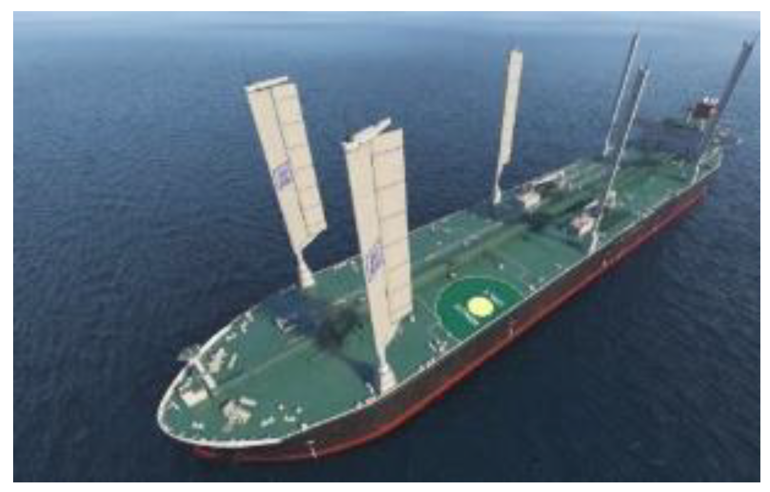
Figure 2.
Kaili ship built by the Dazhang Group.
Figure 2.
Kaili ship built by the Dazhang Group.
Figure 3.
Wing Sail Mobility (WISAMO) system.
Figure 3.
Wing Sail Mobility (WISAMO) system.
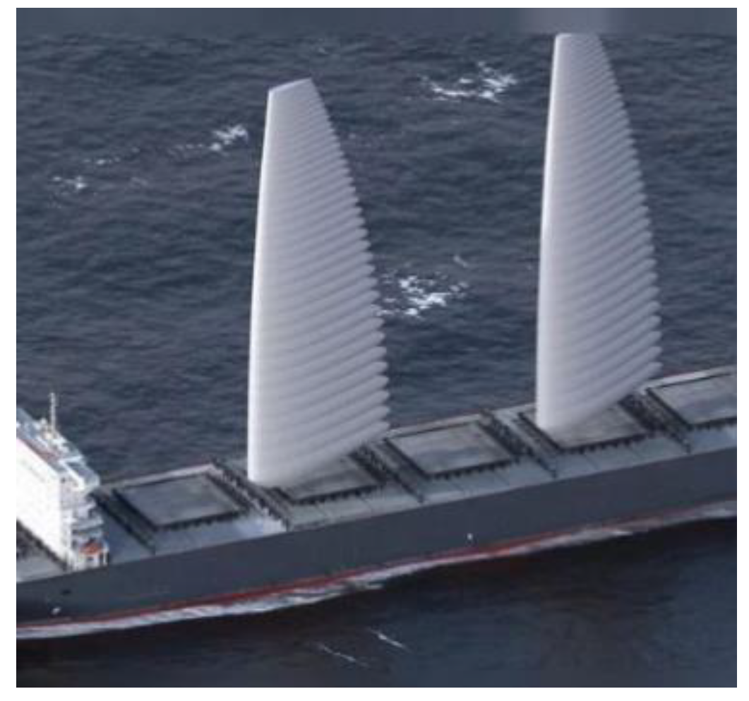
Figure 4.
“Wind Challenger” developed by Mingcun shipbuilding.
Figure 4.
“Wind Challenger” developed by Mingcun shipbuilding.
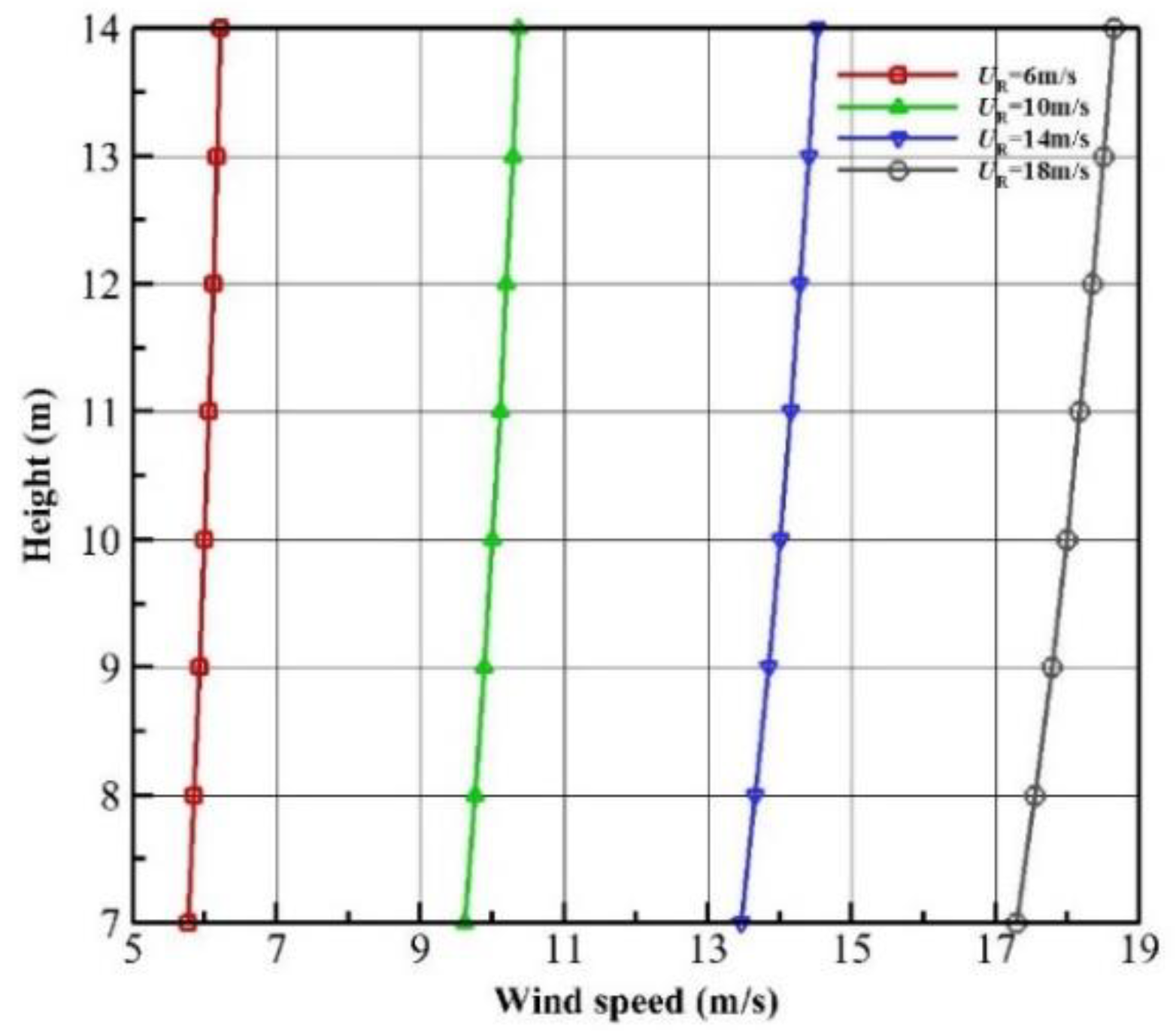
Figure 5.
Mathematical model of wind gradient under different reference wind speeds ( = 10 m, = 0.001 m).
Figure 5.
Mathematical model of wind gradient under different reference wind speeds ( = 10 m, = 0.001 m).
Figure 6.
Mathematical model of wind gradient under different roughness factors ( = 10 m, = 10 m/s).
Figure 6.
Mathematical model of wind gradient under different roughness factors ( = 10 m, = 10 m/s).
Figure 7.
Mathematical model of wind gradient under different reference wind speeds ( = 10 m, p = 0.143).
Figure 7.
Mathematical model of wind gradient under different reference wind speeds ( = 10 m, p = 0.143).
Figure 8.
Mathematical model of wind gradient under different exponential parameters ( = 10 m, = 10 m/s).
Figure 8.
Mathematical model of wind gradient under different exponential parameters ( = 10 m, = 10 m/s).
Figure 9.
Comparison of two models of wind gradient under typical parameter settings.
Figure 9.
Comparison of two models of wind gradient under typical parameter settings.
Figure 10.
Schematic diagram of a certain height from the root of wingsails to the deck.
Figure 10.
Schematic diagram of a certain height from the root of wingsails to the deck.
Figure 11.
Calculation domain of a two-elements wingsail.
Figure 11.
Calculation domain of a two-elements wingsail.
Figure 12.
Mesh details of wingsail surface. (a) Wingsail surface grid structure. (b) Boundary layer grid of the two-elements wingsail.
Figure 12.
Mesh details of wingsail surface. (a) Wingsail surface grid structure. (b) Boundary layer grid of the two-elements wingsail.
Figure 13.
Cloud of y+ on the surface of the wingsail at α = 6°.
Figure 13.
Cloud of y+ on the surface of the wingsail at α = 6°.
Figure 14.
Design framework and experimental model of the AC72 wingsail wind tunnel experiment. (a) Design Framework of the AC72 wingsail experiment. (b) AC72 wingsail experimental model.
Figure 14.
Design framework and experimental model of the AC72 wingsail wind tunnel experiment. (a) Design Framework of the AC72 wingsail experiment. (b) AC72 wingsail experimental model.
Figure 15.
Pressure coefficient of main wing in different sections of the AC72 wingsail. (a) z/h = 0.5, (b) z/h = 0.75.
Figure 15.
Pressure coefficient of main wing in different sections of the AC72 wingsail. (a) z/h = 0.5, (b) z/h = 0.75.
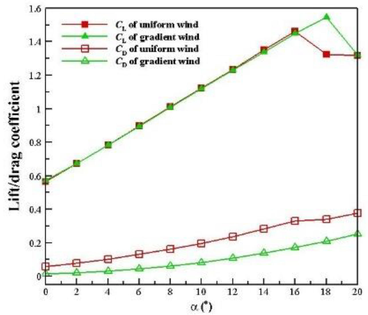
Figure 16.
Lift-drag characteristic of the wingsail under mean wind and gradient wind conditions.
Figure 16.
Lift-drag characteristic of the wingsail under mean wind and gradient wind conditions.
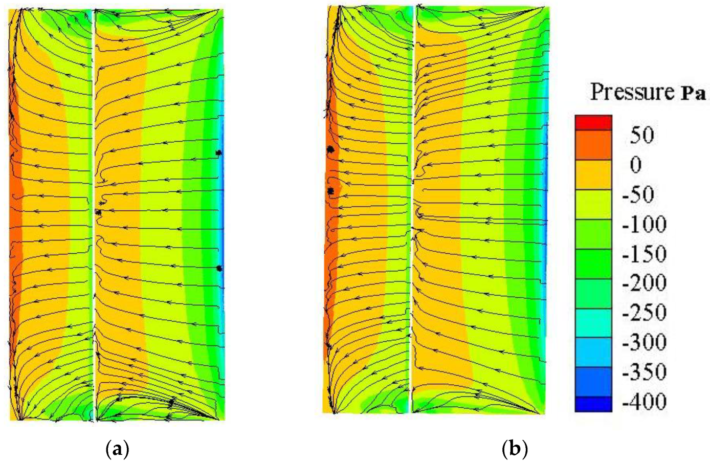
Figure 17.
Wall limiting streamline of the wingsail under uniform wind and gradient wind conditions. (a) Uniform wind at α = 16°. (b) Gradient wind at α = 16°. (c) Uniform wind at α = 18°. (d) Gradient wind at α = 18°.
Figure 17.
Wall limiting streamline of the wingsail under uniform wind and gradient wind conditions. (a) Uniform wind at α = 16°. (b) Gradient wind at α = 16°. (c) Uniform wind at α = 18°. (d) Gradient wind at α = 18°.
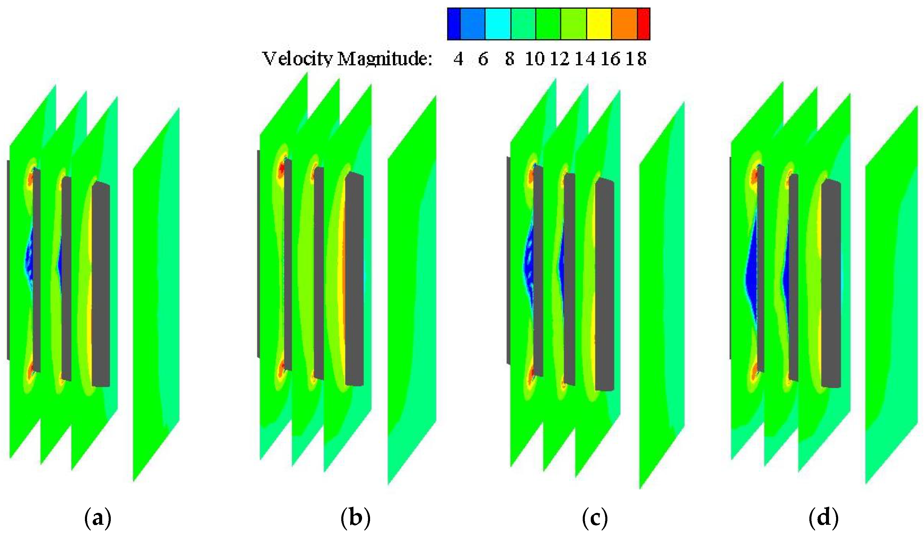
Figure 18.
Velocity distribution of a two-element wingsail under uniform wind and gradient wind conditions. (a) Case 3 with uniform wind at α = 18°. (b) Case 3 with gradient wind at α = 18°. (c) Case 3 with uniform wind at α = 20°. (d) Case 3 with gradient wind at α = 20°.
Figure 18.
Velocity distribution of a two-element wingsail under uniform wind and gradient wind conditions. (a) Case 3 with uniform wind at α = 18°. (b) Case 3 with gradient wind at α = 18°. (c) Case 3 with uniform wind at α = 20°. (d) Case 3 with gradient wind at α = 20°.
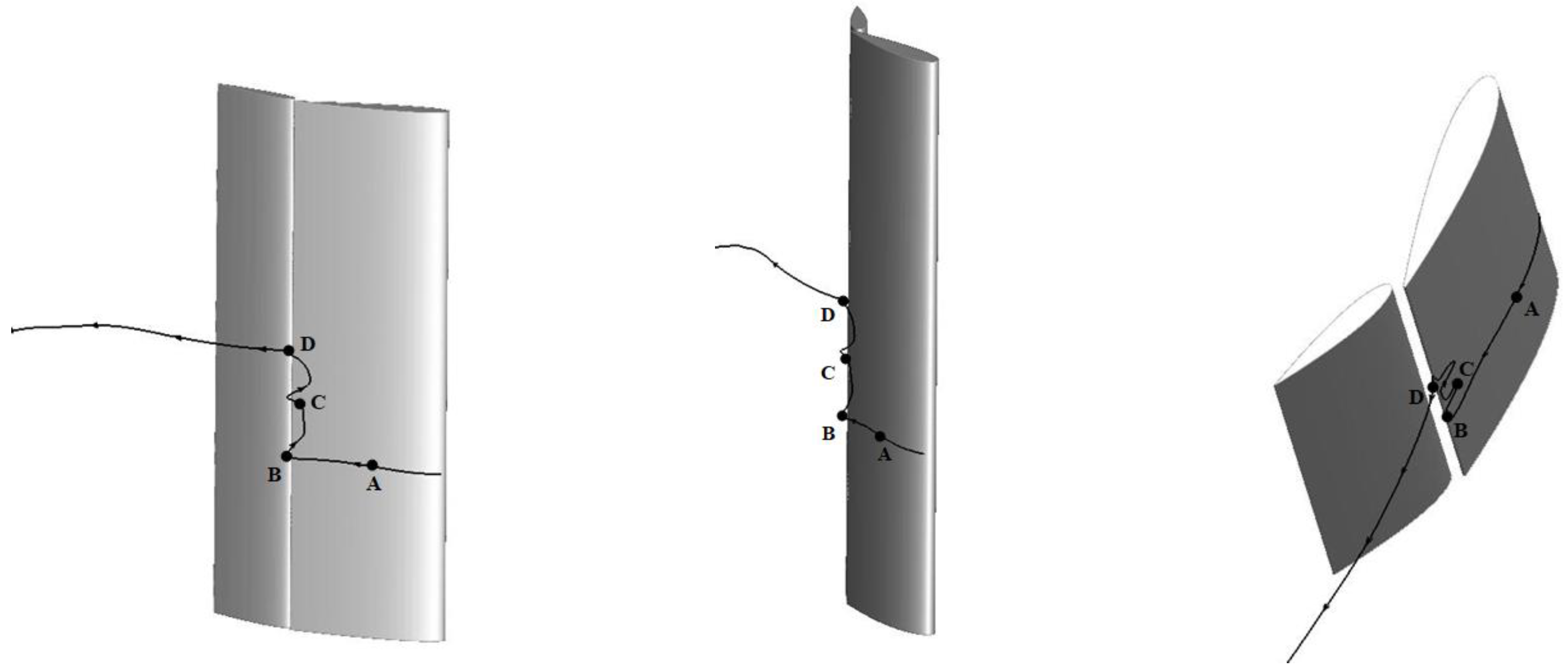
Figure 19.
Three-dimensional streamline of a two-element wingsail under uniform wind and gradient wind conditions. (a) Case 3 with uniform wind at α = 18°. (b) Case 3 with gradient wind at α = 18°. (c) Case 3 with uniform wind at α = 20°. (d) Case 3 with gradient wind at α = 20°.
Figure 19.
Three-dimensional streamline of a two-element wingsail under uniform wind and gradient wind conditions. (a) Case 3 with uniform wind at α = 18°. (b) Case 3 with gradient wind at α = 18°. (c) Case 3 with uniform wind at α = 20°. (d) Case 3 with gradient wind at α = 20°.
Figure 20.
Curve of lift/drag coefficient vs. flap deflection angle in stall angles.
Figure 20.
Curve of lift/drag coefficient vs. flap deflection angle in stall angles.
Figure 21.
Streamline of the two-element wingsail under different flap deflection angles. (a) δ = 19°. (b) δ = 23°. (c) δ = 25°. (d) δ = 27°.
Figure 21.
Streamline of the two-element wingsail under different flap deflection angles. (a) δ = 19°. (b) δ = 23°. (c) δ = 25°. (d) δ = 27°.
Figure 22.
Three-dimensional streamline of the two-elements wingsail at angle of attack of 16°. (a) δ = 19°. (b) δ = 23°. (c) δ = 25°. (d) δ = 27°.
Figure 22.
Three-dimensional streamline of the two-elements wingsail at angle of attack of 16°. (a) δ = 19°. (b) δ = 23°. (c) δ = 25°. (d) δ = 27°.
Figure 23.
A three-dimensional streamline with flap deflection angle of 25° under gradient wind conditions.
Figure 23.
A three-dimensional streamline with flap deflection angle of 25° under gradient wind conditions.
Figure 24.
Mathematical models of wind gradient under different wind speeds ( = 10 m, = 0.001 m).
Figure 24.
Mathematical models of wind gradient under different wind speeds ( = 10 m, = 0.001 m).
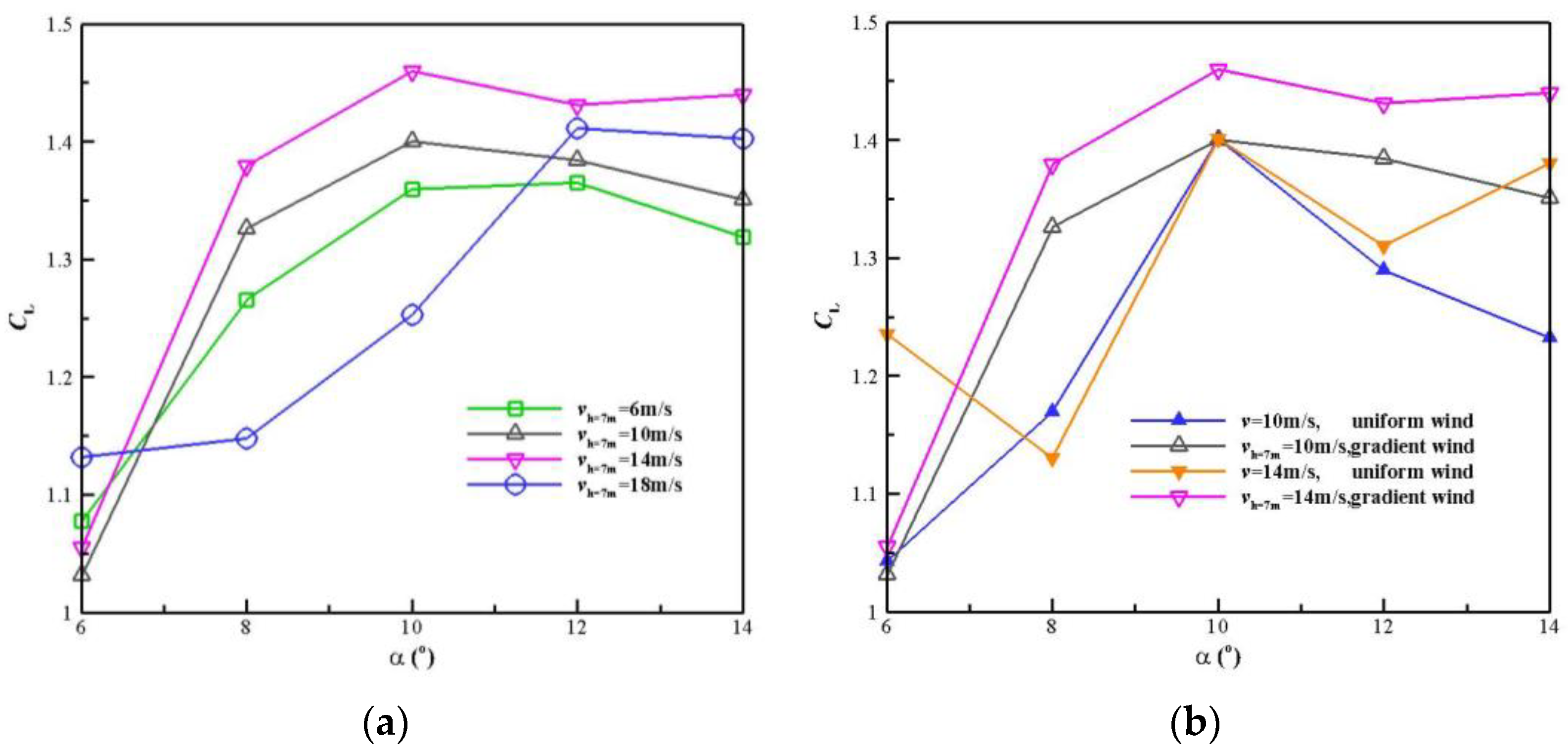
Figure 25.
Curve of lift coefficient with wind average speed under different conditions. (a) Conditions of gradient wind. (b) Conditions of gradient wind and uniform wind.
Figure 25.
Curve of lift coefficient with wind average speed under different conditions. (a) Conditions of gradient wind. (b) Conditions of gradient wind and uniform wind.
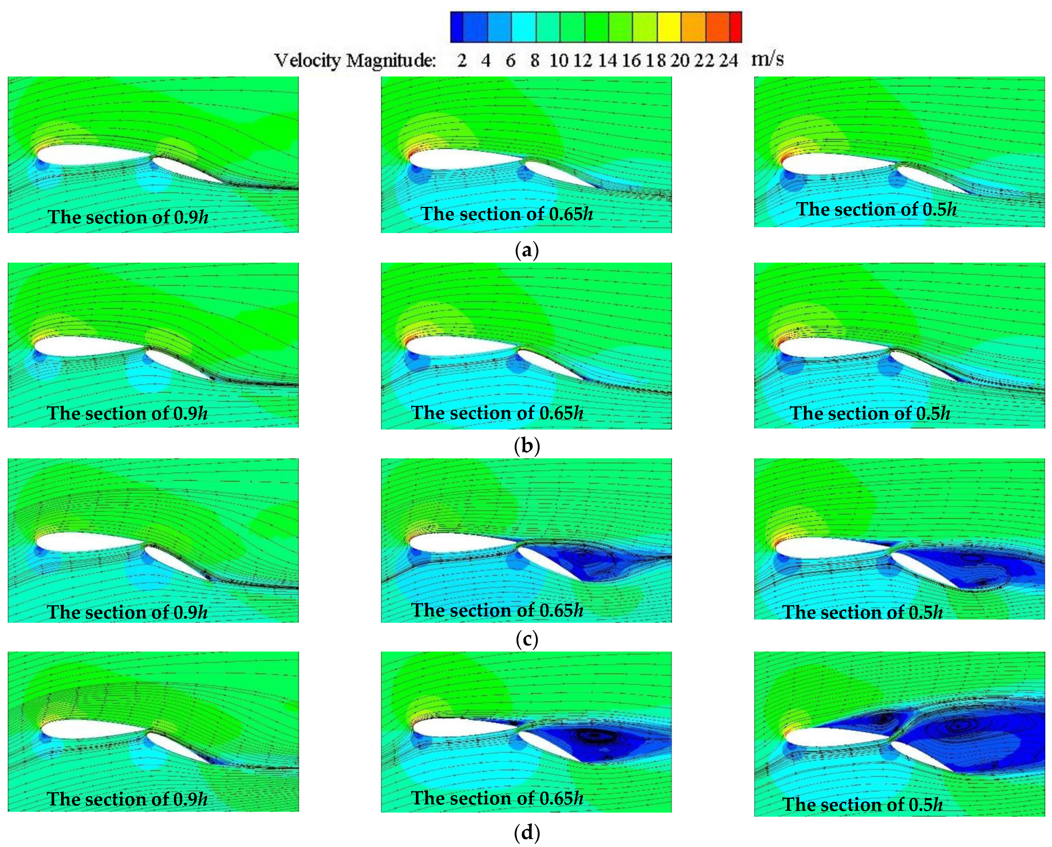
Figure 26.
Limiting streamline of the wingsail under different average wind speeds. (a) v = 6 m/s. (b) v = 10 m/s. (c) v = 14 m/s. (d) v = 18 m/s.
Figure 26.
Limiting streamline of the wingsail under different average wind speeds. (a) v = 6 m/s. (b) v = 10 m/s. (c) v = 14 m/s. (d) v = 18 m/s.
Figure 27.
Speed cloud of wingsail at different average wind speeds at α = 10°. (a) v = 6 m/s. (b) v = 10 m/s. (c) v = 14 m/s. (d) v = 18 m/s.
Figure 27.
Speed cloud of wingsail at different average wind speeds at α = 10°. (a) v = 6 m/s. (b) v = 10 m/s. (c) v = 14 m/s. (d) v = 18 m/s.
Table 1.
Setting of wingsail surface grid parameters.
Table 1.
Setting of wingsail surface grid parameters.
| Grid Type | Grid Size of Wingsail Surface | Total Number of Grids |
|---|
| Coarse grid | 0.8%c | 1.045 × 10⁷ |
| Finer grid | 0.4%c | 1.453 × 10⁷ |
| Thinnest grid | 0.25%c | 1.883 × 10⁷ |
Table 2.
Grid sensitivity analysis at α = 6°.
Table 2.
Grid sensitivity analysis at α = 6°.
| Type | ID | CL | Error (%) | CD | Error (%) |
|---|
| Thinnest grid | φ1 | 1.8210 | — | 0.1516 | — |
| Finer grid | φ2 | 1.8216 | 0.033 | 0.1513 | −0.1979 |
| Coarse grid | φ3 | 1.8193 | −0.093 | 0.1522 | 0.3958 |
| RG | — | 0.2826 | — | 0.3113 | — |
Table 3.
The calculated value of the dispersion error of CL and CD.
Table 3.
The calculated value of the dispersion error of CL and CD.
| Parameter | CL | CD |
|---|
| r32 | 2.05 | 2.05 |
| r21 | 1.63 | 1.63 |
| φ1 | 1.8210 | 0.1516 |
| φ2 | 1.8216 | 0.1513 |
| φ3 | 1.8193 | 0.1522 |
| φ4 | 1.8185 | 0.1525 |
| p | 2.531 | 3.3679 |
| φext21 | 0.2742 | 0.1408 |
| ea21 | 0.528% | 0.453% |
| eext21 | 0.613% | 0.227% |
| GCIfine21 | 0.669% | 0.362% |
Table 4.
Design parameters of AC72 wingsail model.
Table 4.
Design parameters of AC72 wingsail model.
| Height | 1.8 m |
|---|
| Total chord length of blade root | 0.5 m |
| Reynolds number of blade root | 6.4 × 10⁵ |
| Reynolds number of the blade tip | 2.9 × 10⁵ |
| Gap width | 6 mm |
| Flap rotation axis position | 95%c1 |
| Flap deflection angle | 0–25° |
| Angle of attack | 0–16° |
| The maximum speed in the duct | 42 m/s |
| The airfoil of the main wing | NACA0025 |
| The airfoil of the flap | NACA0012 |
Table 5.
Transition position and separation bubble length of suction surface of AC72.
Table 5.
Transition position and separation bubble length of suction surface of AC72.
| | Separation Position of Separation Bubble(/%c1) | Length of Separation Bubble (/%c1) |
|---|
| CFD | TEST | Error | CFD | TEST | Error |
|---|
| z/h = 0.25 | 34 | 39.5 | −13.92% | 14 | 12.5 | 12% |
| z/h = 0.5 | 30 | 32 | −6.25% | 18 | 16 | 12.5% |
| z/h = 0.75 | 31 | 36 | −13.89% | 17 | 15 | 13.33% |


