Article

Research on the Multi-Equipment Cooperative Scheduling Method of Sea-Rail Automated Container Terminals under the Loading and Unloading Mode

1
Institute of Logistics Science and Engineering, Shanghai Maritime University, Shanghai 201306, China
2
China Mobile (Shanghai) Information Communication Technology Co., Ltd., Shanghai 201306, China
*
Author to whom correspondence should be addressed.
J. Mar. Sci. Eng. 2023, 11(10), 1975; https://doi.org/10.3390/jmse11101975
Submission received: 8 September 2023 / Revised: 25 September 2023 / Accepted: 10 October 2023 / Published: 12 October 2023
(This article belongs to the Special Issue Recent Advances in Intelligent Port Logistics)

Abstract

:
A sea-rail automated container terminal (SRACT) plays a crucial role in the global logistics network, combining the benefits of sea and railway transportation. However, addressing the challenges of multi-equipment cooperative scheduling in terminal and railway operation areas is essential to ensure efficient container transportation. For the first time, this study addresses the cooperative scheduling challenges among railway gantry cranes, yard cranes, and automated guided vehicles (AGVs) under the loading and unloading mode in SRACTs, ensuring efficient container transportation. This requires the development of a practical scheduling model and algorithm. In this study, a mixed integer programming model was established for the first time to study the multi-equipment cooperative scheduling problem of a SRACT under the loading and unloading mode. A self-adaptive chaotic genetic algorithm was designed to solve the model, and the practicability and effectiveness of the model and algorithm were verified by simulation experiments. Furthermore, this study also proposes an AGV number adjustment strategy to accommodate changes in vessel arrival delays and train container types. Simulation experiments demonstrated that this strategy significantly reduces loading and unloading time, decreases equipment energy consumption, and improves the utilization rate of AGVs. This research provides valuable guidance for ongoing SRACT projects and advances and methodological approaches in multi-equipment co-operative scheduling for such terminals.

1. Introduction

According to data released by the United Nations Conference on Trade and Development, over 80% of global trade is transported by ships [1]. Implementing automated container terminals has become an inevitable trend in transforming ports worldwide, owing to their efficiency, safety, and reduced reliance on manual labor [2]. As reported in the Alphaliner report for 2021, all of the top 10 container terminals have either operational or under-construction automated container terminals [3]. Using the sea-rail mode can yield cost savings of 10–30% compared to the single sea mode, primarily due to enhanced efficiency and lower transport costs associated with this mode [4]. Several studies, such as [5,6,7,8,9,10], have analyzed the advantages and disadvantages of integrating rail transport with other modes and have highlighted the sea-rail mode as a future development trend that requires urgent attention.
To build an efficient sea-rail automated container terminal (SRACT), in addition to solving the problem of industrial IoT [11,12,13], there is also a need to solve the problem of coordinated scheduling of multiple equipment between the two sides. In a SRACT, the interface between the yard crane (YC) and the quay crane (QC) within the terminal is not the only consideration; it also involves coupling with the railway track crane. Consequently, a SRACT encompasses the container and traffic flow between the ship and the yard and the container and traffic flow between the rail-mounted gantry cranes (RGCs) and the YC, and between the RGCs and the QC. Traffic flow is always an important research object in the field of traffic [14]. The arrival of vessels at the port may be delayed due to factors such as inclement weather and port congestion, which can significantly disrupt the loading and unloading schedule of a SRACT. In this study, we delve into the integrated scheduling challenge faced by RGCs, YCs, and automated guided vehicles (AGVs) during the processes of loading and unloading at SRACTs, with the objective of optimizing container transport efficiency. The contributions of this paper are as follows:
(1)
This study is the first to investigate the collaborative scheduling problem under the loading and unloading mode in SRACTs, filling a research gap in this domain and holding immense practical significance for the construction and operation of SRACTs.
(2)
Six container flows and seven AGV flows under the loading and unloading mode are proposed, offering clear operational guidance and a classification system for collaborative scheduling within SRACTs.
(3)
Based on the flow classification, a mathematical model for multi-device cooperative scheduling under the loading and unloading mode in SRACTs is established, and a heuristic algorithm is devised to obtain approximate optimal solutions for the model without pursuing the exact optimal solution.
(4)
In the face of common real-world scenarios such as delayed arrival of ships and variations in the types of containers on trains, AGV adjustment strategies are designed to meet the actual scheduling needs of SRACTs, enhancing the practicality of the research.
The significance of this study is many fold, addressing both theoretical and practical aspects of operations within SRACTs. Theoretically, this research provides a foundational framework for the operation of SRACTs with the layout as shown in Figure 1, extending its implications for sea-rail intermodal automated container terminals with various other layouts. This new methodological framework enriches the existing body of knowledge in the field of sea-rail intermodal terminals and is poised to serve as a significant reference for subsequent related research. Practically, the introduction of the proposed flow classification, mathematical models, and solving algorithms enables more efficient collaborative scheduling of equipment within SRACTs, substantially enhancing the overall operational efficiency of the terminal. Furthermore, the studied AGV adjustment strategies hold substantial application value for addressing real-world scenarios such as delayed ship arrivals and variations in container types on trains, offering effective solutions to practical problems encountered in terminal operations.
The remainder of this paper is as follows: Section 2 provides a review of the corresponding references. Section 3 analyzes the operation flow of the SRACT based on the loading and unloading mode and proposes a collaborative scheduling model for multiple equipment. Section 4 designs a suitable algorithm for the model. Section 5 conducts numerical experiments and performs an equipment rationing analysis. Conclusions are given in Section 6.

2. Literature Review

In the global logistics field, sea-rail intermodal transportation of containers has emerged as a significant development trend, leading to increased attention on the multi-equipment cooperative scheduling problem in SRACTs. This chapter aims to review relevant research on equipment scheduling in automated container terminals and equipment scheduling in sea-rail intermodal terminals, providing valuable references and guidance for this study.

2.1. Scheduling Study of AGVs and YCs in Automated Container Terminals

One area of current research that has focused on scheduling equipment in automated container terminals is scheduling AGVs and YCs. The AGVs transport containers within the horizontal transport zone between the terminal front and the yard [15]. The YC is strategically positioned in the yard to handle container loading and unloading from the AGV and external trucks and manage container space in the yard.
Zhou et al. [16] and Iris et al. [17] reviewed AGV use in green ports. Several studies [18,19,20,21,22,23] have focused on reducing the operation time and waiting time of AGVs. Other studies [24,25,26] have investigated YC scheduling rules and travel paths. In addition, research efforts [27,28,29,30] have explored the scheduling problem of multiple YCs, considering mutual interference and safety distance between YCs.
While the above studies address individual equipment aspects of AGVs and YCs, an automated container terminal is a complex system where each operation link impacts others. Therefore, studying the synergistic scheduling of AGVs and YCs is crucial for enhancing port production efficiency.
Zhang et al. [31] considered yard buffer capacity constraint and the interference problem of dual YCs and developed a cooperative dispatching model for AGVs and YCs in the YC relay mode. Yang and Jiang et al. [32] described a scenario involving interior yard entry with the assistance of ground trolleys to operate cooperatively with the YC. Chen et al. [33] addressed the integrated scheduling problem of YCs and AGVs as a multi-robot coordinated scheduling problem, proposing a multi-commodity network flow model with two sets of flow balance constraints. Hsu et al. [34] employed four heuristic algorithms to tackle the cooperative scheduling problem of the YC and trucks and showed that the hybrid algorithm outperformed others. Zhou et al. [35] conducted a pioneering study of vehicles on both sides of the container area during YC operations in automated container terminals and described the YC motion process of side loading and unloading. Furthermore, studies by [36,37,38] utilized simulation approaches to examine the effects of terminal layout and equipment configuration on energy consumption. Iris et al. [39] optimized the energy consumption of equipment at ports.
In summary, scholars have conducted comprehensive research on the collaborative scheduling of AGVs and YCs, and have proposed numerous effective scheduling optimization methods that strongly support the investigation of automated container terminals for sea-rail transportation. However, the majority of studies have primarily focused on the operational or waiting times of individual equipment. These isolated investigations do not adequately address the integrated nature of port systems where various operational processes are interdependent. Consequently, even though some studies, such as [23,24,25,26], have taken into consideration coordinated scheduling, there appears to be a lack of comprehensive exploration into the actual benefits and challenges of implementing such collaborations. Furthermore, research concerning AGVs and YCs seems to overlook discussions on simultaneously ensuring environmental sustainability and energy efficiency, indicating that a multi-device, bi-objective study is a direction that warrants special consideration.

2.2. Equipment Scheduling at Sea-Rail Terminals

Due to differing operational procedures and rules between railway operation areas and automated container terminals, relevant research findings from automated container terminals cannot be directly applied to railway operation areas of automated container terminals in SRACT. Some scholars have conducted detailed research on railway operation areas.
Ballis and Golias [40] provided insights into the layout of railway operation areas, enhancing researchers’ understanding of equipment scheduling problems in this context. Boysen et al. [6] delved into the operations research perspective and analyzed fundamental decision problems related to traditional railway–road and modern railway–railway transfer yards when handling containers. Wang and Zhu [9] optimized the operation sequence of RGCs during loading and unloading to minimize the RGC idling time. Li et al. [41] focused on single-machine scheduling of RGCs and introduced the moving time window constraint, laying the foundation for addressing the scheduling problem of multiple RGCs. Li et al. [10] and Ren et al. [42] studied the collaborative optimization problem of multiple RGCs and internal trucks and proposed reduced interactions between two RGCs through internal truck transportation to minimize the long-distance full-load movement of RGCs.
However, most of these studies solely considered equipment scheduling within the railway operation area and overlooked the need for cooperation between equipment in the railway operation area and the terminal. Some scholars have examined multi-equipment synergistic scheduling issues in non-automated terminals for sea-rail intermodal transport. Yan et al. [43] investigated the collaborative scheduling problem of RGCs, internal collector trucks, and stacker cranes and validated the effectiveness of the developed model using different algorithms. Chang et al. [44] explored container storage rules in a railway station during train unloading to reduce the overturning operation of RGCs. However, these studies have primarily focused on export containers and have neglected the container flow of imported containers and containers transported to the yard.
In SRACTs, Li et al. [8] proposed a cluster scheduling method for multi-IGVs between terminal yards and railway yards by grouping RGCs, AGVs, and YCs and performed cluster scheduling while considering non-crossing and safety distance constraints. Although this cluster dispatching method somewhat reduced dispatching complexity, it sacrificed vehicle flexibility. Additionally, their study needed to address the coupling of loading and unloading tasks between trains and ships, necessitating further investigation. Yang et al. [7] investigated the synergistic relationship between RGCs and AGVs in an automated sea-rail container terminal and explored the impact of the number of RGCs and AGVs on total equipment energy consumption. However, their study only considered export container operation mode and overlooked import container cases. Furthermore, the study needed to account for the operation time of the YC, which still has limitations.
However, most of the aforementioned studies on sea-rail terminals have tended to treat railway operations and container terminal operations as two distinct entities. This situation implies a significant research gap, namely, how to coordinate the scheduling of various equipment in an automated SRACTs environment. While the study by Ballis and Golias [35] proposed a clustering scheduling method, it compromised the flexibility of vehicles. In practical operations, the ability to swiftly adapt to changes and uncertainties is paramount. Moreover, the research by Li et al. [36], although it addressed the synergy between RGCs and AGVs, overlooked the operating patterns of inbound containers, which are crucial for ensuring overall efficiency and fluidity.

2.3. Research Overview

Upon review of the literature, while existing research has explored the multi-device scheduling of SRACTs from perspectives such as constraint conditions, modeling techniques, and algorithmic thinking, it has provided useful references for this paper’s research but still has the following limitations:
(1)
Most research has been focused on single scenarios of automated terminals or railway operation areas, failing to fully reflect the strong coupling between port operations and railway operations. There is a need to investigate the interrelations between multiple devices involved in SRACTs, with a focus on the flow direction of containers and vehicles.
(2)
Existing studies on sea-rail intermodal collaborative scheduling have only considered train unloading modes, lacking research on loading modes, thereby failing to comprehensively reflect the operation process at SRACTs. Thus, it is necessary to consider both unloading and loading operations of trains in the multi-device collaborative scheduling method for SRACTs, given complex container and vehicle flows, to enhance the overall production efficiency of these terminals.
Aiming at the above problems, this paper first analyzes the container flow and vehicle flow involved in the loading and unloading mode of a SRACT. Then, for the first time, a multi-equipment integrated cooperative scheduling model of the SRACT under the loading and unloading mode is established, and the self-adaptive chaotic genetic algorithm is designed to solve the model. Moreover, this paper investigates the adjustment strategy of AGVs under the loading and unloading mode, particularly when ship arrivals are delayed or train container types are changed. The ultimate objective is to enhance the efficiency and capacity of port operations by offering invaluable insights for effectively tackling the practical challenges associated with multi-equipment cooperative scheduling in SRACTs.

3. Model Establishment

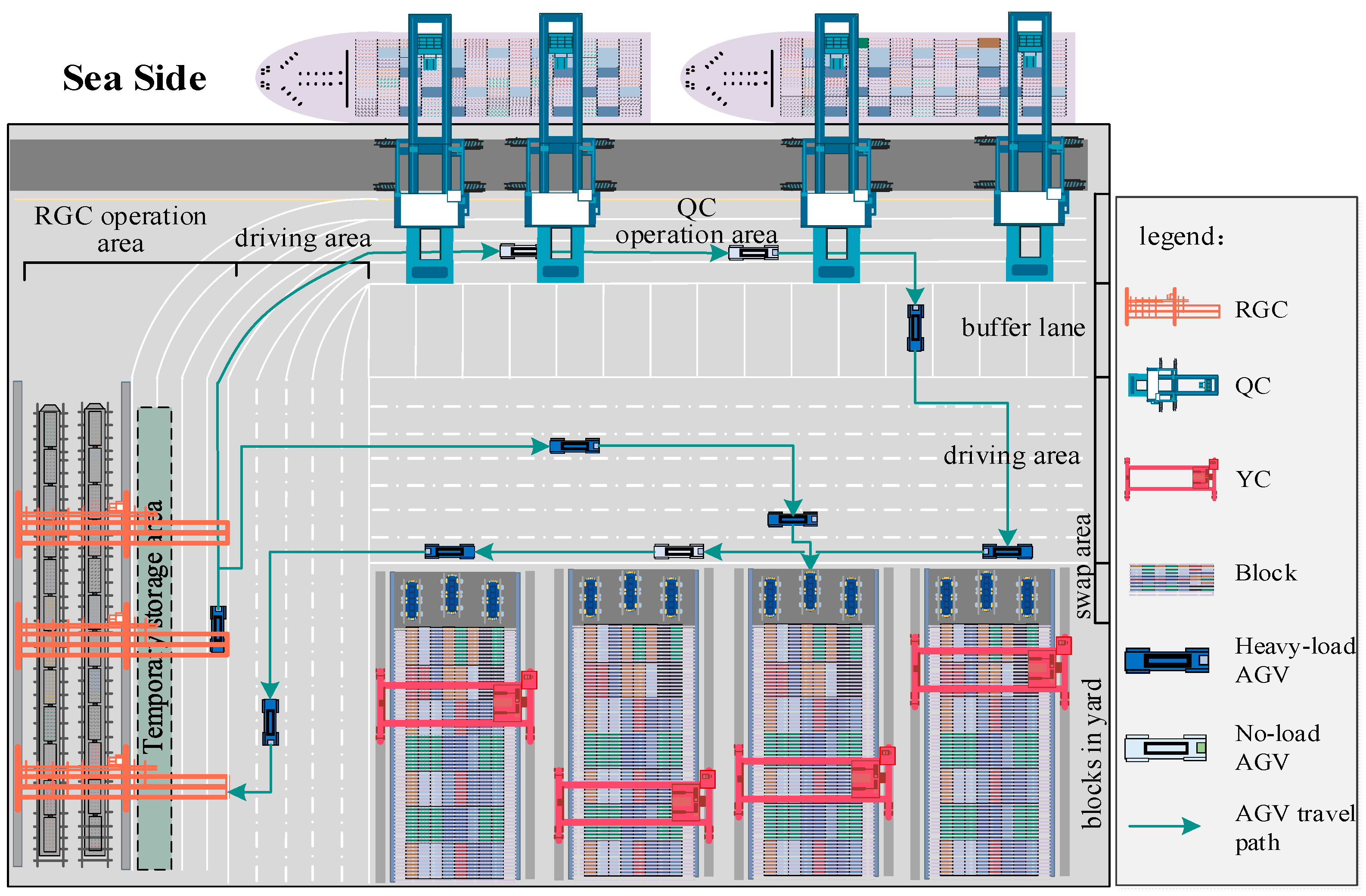
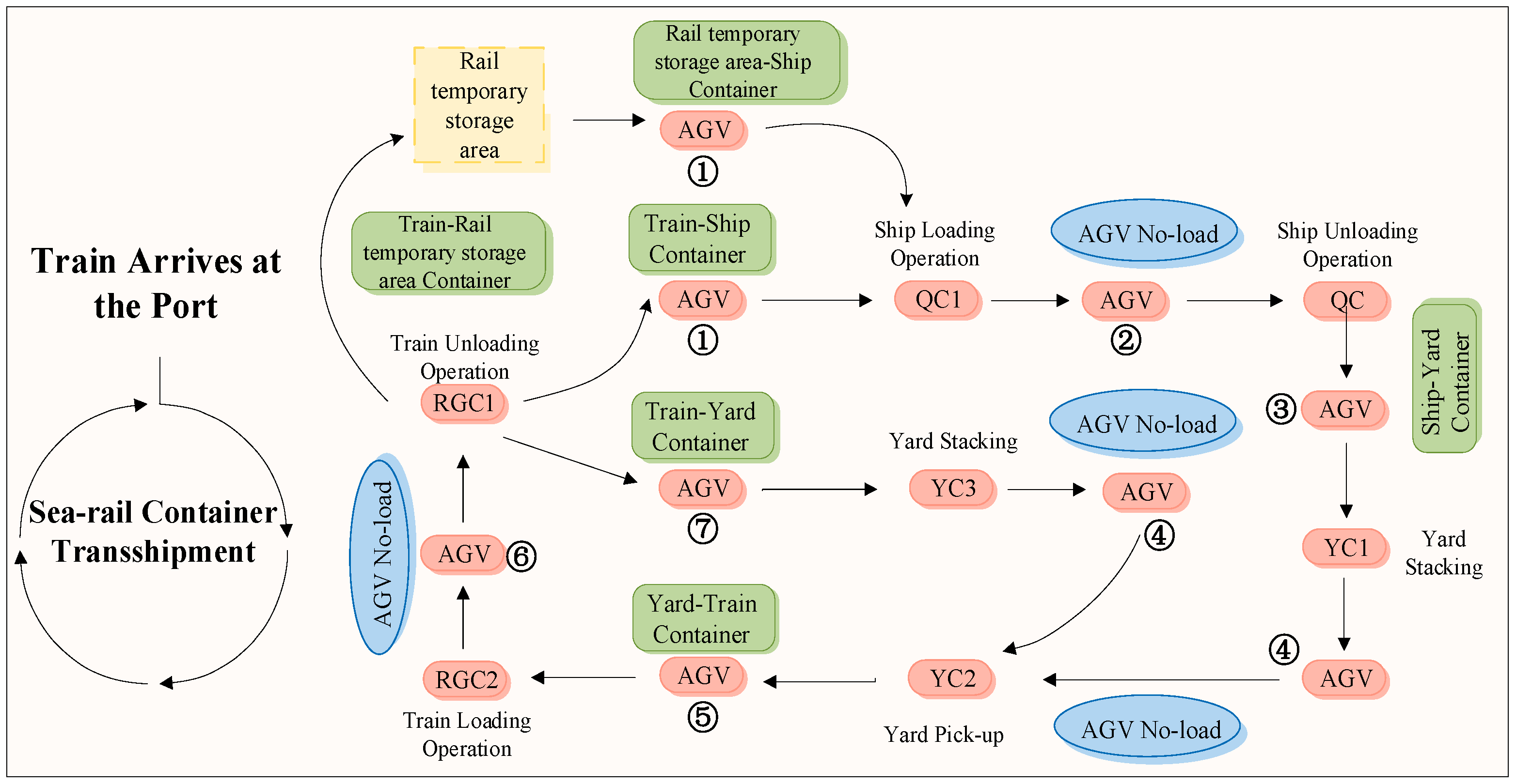
3.1. Analysis of the Operation Process of the SRACT

This study investigates a SRACT characterized by a vertical railway approach and a shared yard that serves both the railway and the terminal. In this terminal layout, railway tracks are arranged vertically to the shoreline on one side of the port, facilitating the entry and exit of trains while reducing conflict with other vehicles. In addition to being stored in the port yard, containers can also be temporarily placed in the railway operation area, with the storage location determined by the attributes of the container. A detailed layout of this port is shown in Figure 1.
At SRACTs, a simultaneous loading and unloading method is adopted to enhance terminal efficiency and AGV utilization, and is described as follows: After an AGV delivers a container to the QC for loading onto a ship, it proceeds to another QC to pick up an unloaded container. Once an AGV has delivered a container to the yard, it goes to another yard to collect a container. After an AGV has taken a container to the RGC for loading onto a train, it proceeds to another RGC to collect a container.
Because the stability of a ship is mainly determined by the ship’s stowage, therefore, containers on the train can be loaded directly onto the ship. However, each train car can only accommodate one container; if the center of gravity of any container is shifted, the train may overturn when turning. Therefore, containers from ships cannot be directly loaded onto trains. The containers must be transferred to the yard first, inspected, and then permitted for loading. Hence, this paper does not consider the flow of containers between ships and trains.
In summary, there are six types of container flows within the SRACT under the loading and unloading mode, namely “train–ship”, “train–rail temporary storage area”, “rail temporary storage area–ship”, “ship–yard”, “train–yard”, and “yard–train”. To transport containers in these six flow directions between RGCs, YCs, and QCs, the AGVs operate in seven flow directions: ① “RGC-QC”, ② “QC-QC”, ③ “QC-YC”, ④ “YC-YC”, ⑤ “YC-RGC”, ⑥ “RGC-RGC”, and ⑦ “RGC-YC”, as illustrated in Figure 2. Based on the above container flow and AGV flow, the SRACT multi-equipment cooperative scheduling model under the loading and unloading mode is established as described below.

3.2. Collaborative Scheduling Optimization Model for Multiple Equipment

This section aims to construct a mixed-integer optimization model to minimize both the total time spent on loading and unloading and the operational energy consumption of RGCs and AGVs. The goal is to find the loading and unloading sequence for RGCs and AGVs that balances efficiency and energy consumption.

3.2.1. Basic Assumptions

Without loss of generality, the following assumptions can be made:
  • All the containers discussed are standard 40-foot containers.
  • The AGVs, YCs, and RGCs can and should only handle one task at a time.
  • The travel speed and energy consumption of the AGVs, as well as the movement speed of the RGCs’ gantry and spreader, are assumed to be constant.
  • The transit time for the RGCs’ spreader to travel vertically between the top and bottom is considered to be a fixed value.
  • The capacity of the YCs’ buffering brackets is set to be a consistent value.
  • The operation time of AGVs under the QC and the time taken for the lifting gears of YCs and RGCs to pick up and place containers from the AGVs are not counted.

3.2.2. Symbol Description

To facilitate modelling, the following sets, parameters, non 0–1 Variables, and 0–1 Variables are defined firstly.

Set

R Set of RGCs, R = 1 , 2 , , r
V Set of AGVs, V = 1 , 2 , , v
Q Set of QCs, Q = 1 , 2 , , q
Z Set of Ycs, Z = 1 , 2 , , z
B Set of train wagons, B = 1 , 2 , , b
E 1 Set of Train-Ship tasks, E 1 = 1 , 2 , , i , j
E 2 Set of Train-Yard tasks, E 2 = 1 , 2 , , i , j
E Set of unloading tasks, E = E 1 E 2 P
P Set of containers requiring temporary storage, P = 0 , 1 , , b B Q α r i p b
I Set of Yard-Train tasks, I = 1 , 2 , , i , j
N Set of train tasks, N = E I
0 Virtual start task of the train,
F Virtual end task of the train,
N 0 N 0 = N 0
N F N F = N F
K Set of Ship-Yard tasks, K = 1 , 2 , , k
φ Set of tasks that cannot be operated by RGCs simultaneously,
φ = ( i , j ) i , j N , l j l i l s a f

Parameters

C 1 Energy consumption of one RGC’s gantry, unit: kWh/h
C 2 Energy consumption of one RGC’s spreader, unit: kWh/h
C 3 Energy consumption of one RGC’s waiting, unit: kWh/h
C 4 Energy consumption of one AGV under loaded condition, unit: kWh/h
C 5 Energy consumption of one AGV under unloaded condition, unit: kWh/h
C 6 Energy consumption of one AGV’s waiting, unit: kWh/h
C E R Total energy consumption of RGCs
C E V Total energy consumption of AGVs
S R Moving speed of RGC’s spreader
S A E Unloaded moving speed of AGVs
S A H Loaded moving speed of AGVs
τ 1 Time for RGC’s spreader to move one wagon bay
τ 2 Average operation time for RGCs to place containers from temporary storage to AGVs
τ 3 Average operation time for Ycs to handle one container
τ 4 Time for the RGC’s spreader to rise/fall
ρ Capacity of yard buffer stands
x i Loading and unloading line position of task i
y i Bay position of the wagon for task i
d r g i Moving distance of RGC r ’s spreader from the loading/unloading line of task i to the AGV operating lane above
d r i p Distance for RGC r to move from the loading/unloading line of task i to the temporary storage area
l s a f Safety distance of RGC
M An infinitely large integer
ω 1 Weight coefficient of completion time of loading/unloading
ω 1 Weight coefficient of total energy consumption of equipment
T s h i p Ship’s arrival time
T E v z i The earliest time AGV v can pick up/drop off task i at the buffer stand under the container area of YC z
T L v z i The latest time AGV v can pick up/drop off task i at the buffer stand under the container area of YC z
D i j Distance from equipment i to equipment j

Non 0–1 Variables

T S r i Time when RGC r starts task i
T P r i Time when RGC r ’s spreader moves to the AGV operating lane above task i
T I r i Time when RGC r starts interacting with AGV for task i
T F r i Time when RGC r completes task i , i.e., time when RGC r loads task i onto the AGV or time when RGC r loads task i onto the train
T Y v i Time when AGV v arrives under YC during task i
T R v i Time when AGV v arrives under RGC during task i
T Q v i Time when AGV v arrives under QC during task i
T E v z i The earliest time AGV v can pick up/drop off task i at the buffer stand under the container area of YC z
T L v z i The latest time AGV v can pick up/drop off task i at the buffer stand under the container area of YC z
T F v i Time when AGV v completes task i
Q α r i p b Number of containers stored in temporary storage area bay b when RGC r is operating task i
t r o i Transversal movement time of RGC r ’s spreader during task i
t v f i Loaded time of AGV v during task i
t v 0 i j Empty time of AGV v after task i and before task
t w v r i Time for RGC r to wait for AGV v during task i
t w v z i Time for YC z to wait for AGV v during task i
t w r v i Time for AGV v to wait for RGC r during task i
t w z v i Time for AGV v to wait for YC z during task i
t v i r z Time for AGV v to transport task i from RGC r to YC z /Time for AGV v to transport task i from YC z to RGC r
t v i r q Time for AGV v to transport task i from RGC r to QC q
t v i q z Time for AGV v to transport task i from QC q to YC z
t v i , j q 1 q 2 Time for AGV v to travel to QC q to pick up task i after completing task i at QC q
t v i , j z r Time for AGV v to travel to RGC r to pick up task j after completing task i at YC z
t v i , j r 1 r 2 Time for AGV v to travel to RGC r to pick up task j after completing task i at RGC r
η Utilization rate of AGV
T u s e f u l Total loaded time of AGV
T t o t a l Total operating time of AGV

0–1 Variables

α r i When RGC r operates task i , α r i = 1 , otherwise α r i = 0
β v i When AGV v operates task i , β v i = 1 , otherwise β v i = 0
w r i j When RGC r operates task i and continues to task j , w r i j = 1 , otherwise w r i j = 0
w v i j When AGV v operates tasks i and j consecutively, w v i j = 1 , otherwise w v i j = 0
w z i j When YC z operates tasks i and j consecutively, w z i j = 1 , otherwise w z i j = 0
λ r v i When task i is operated by RGC r and AGV v , λ r v i = 1 , otherwise λ r v i = 0
μ v z i When task i is operated by AGV v and YC z , μ v z i = 1 , otherwise μ v z i = 0
γ v q i When task i is operated by AGV v and QC q , γ v q i = 1 , otherwise γ v q i = 0
ψ i When RGC r operates task i in the temporary storage area, ψ i = 1 , otherwise ψ i = 0

3.3. Cooperative Scheduling Model of RGCs, AGVs, and YCs

min f = ω 1 · f 1 + ω 1 · C E R + C E V
f 1 = max r R T F r i , i N
C E R = r R i N C 1 α r i t r o i + r R i , j N C 2 w r i j y j y i τ 1 + r , r R v V i , j N C 3 λ r v i t w v r i
C E V = v V i N C 4 β v i t v f i + v V i , j N C 5 w v i j t v 0 i j + v V i N z Z C 6 ( λ r v i t w r v i + μ v z i t w z v i )
Equation (1) represents the objective function, which is the sum of the weighted value of the maximum completion time and the operational energy consumption of the RGCs and AGVs. Equation (2) represents the maximum completion time. Equation (3) calculates the total operational energy consumption of the RGCs, including the loading and unloading energy consumption of the YCs’ gantry and spreader, the movement energy consumption of the gantry, and the RGC waiting for the AGV. Equation (4) calculates the total operational energy consumption of AGVs, which includes the energy consumed under heavy load, no load, and during the waiting period under the RGCs and YCs.
r R α r i = 1 , i N
i N α r i = 1 , r R
i N F w r 0 i = 1 , r R
i N 0 w r i F = 1 , r R
j N F , j i w r i j j N 0 , j i w r j i = 0 , r R , i R
v V β v i = 1 , i N K
i N K β v i = 1 , v V
i N F K , j i w r 0 i = 1 , v V
i N 0 K , j i w r i F = 1 , v V
j N F K , j i w v i j j N 0 K , j i w v j i = 0 , v V , i R
Equations (5)–(14) denote the uniqueness constraints for equipment operation. Specifically, Equation (5) signifies that each task is handled by one and only one RGC, while Equation (6) ensures that each RGC can operate on one task, and only one task, at any given time. Equations (7)–(9) are set up to ensure that a singular predecessor and successor task is associated with each RGC. Similarly, Equation (11) dictates that each task is serviced by exactly one AGV. In contrast, Equation (12) ensures that an AGV is assigned a single task and no more. Finally, from Equations (13) to (15), it is stipulated that an unbroken chain of predecessor and successor tasks is maintained for every AGV.
T S r j > T F r i + l s a f · τ 1 , r , r R , ( i , j ) φ
T S r i + 2 τ 4 + d r g i / S R T P r i + ( 1 α r i ) M , r R , i N
t r o j = w r i j ( 3 τ 4 + d r g i / S R ) , i E , j I , r R w r i j ( 4 τ 4 + x i x j / υ + d r g i / S R ) , i I , j E , r R
T P r i + τ 4 T I r i + ( 1 α r i ) M , r R , i N
T F r i = T I r i + ( 1 α r i ) M , r R , i N
Q α r i p b = Q α r i p b + 1 ,   if   T S r i < T s h i p Q α r i p b , e l s e , i E 1 , r R , b B
T F r i + τ 4 + y i y j · τ 1 T S r j + ( 1 w r i j ) M , i E , j I , r R
T F r i + τ 4 + ψ i d r i p + ( 1 ψ i ) x i x j · υ + y i y j · τ 1 T S r j + ( 1 w r i j ) M i I , j E , r R
Equation (15) stipulates a constraint that the distance between any two adjacent RGCs, at any given time, must exceed the safety distance. Equation (16) establishes the relationship between the moment RGC r starts operating the task i and the moment the spreader of RGC r moves above the AGV operation lane. Equation (17) calculates the time taken by the spreader of RGC r to operate task i . Equation (18) establishes the relationship between the moment when the spreader of RGC r moves above the AGV operation lane and when RGC r starts interacting with the AGV in the operation task i . Equation (19) represents the end moment of task i . Equation (20) corresponds to the scenario when a ship’s arrival is delayed, requiring temporary storage of the train–ship task i in the corresponding bay b of the temporary storage area. Equation (21) represents the relationship between the completion moment of the previous unloading task i operated by RGC r and the start moment of the next loading task j . Equation (22) represents the relationship between the completion moment of the previous loading task i operated by RGC r and the start moment of the next unloading task j .
t v i r z = D r z / S A H , i E 2 I , r R , v V , z Z
t v i r q = D r q / S A H , i E 1 P , r R , v V , q Q
t v i q z = D q z / S A H , i k , v V , z Z , q Q
t v f i = t v i r z , i E 2 I , r R , v V , z Z t v i r q , i E 1 P , r R , v V , q Q t v i q z , i k , v V , z Z , q Q
t v i , j q 1 q 2 = D q 1 q 2 / S A E , i E 1 , j K , v V , q 1 Q , q 2 Q
t v i , j z r = D z r / S A E , i E 2 K , j I , v V , z Z , r R
t v i , j r 1 r 2 = D r 1 r 2 / S A E , i I , j E , v V , r 1 R , r 2 R
t v 0 i j = t v i , j q 1 q 2 , i E 1 , j K , v V , q 1 Q , q 2 Q t v i , j z r , i E 2 K , j I , v V , z Z , r R t v i , j r 1 r 2 , i I , j E , v V , r 1 R , r 2 R
Equation (23) outlines the duration for AGV v to transport the “train–yard” and “yard–train” tasks i between the RGC and YC. Equation (24) represents the time it takes for AGV v to handle the “train–ship” task i between the RGC and QC. Equation (25) illustrates the time duration during which AGV v transports the “ship–yard” task i from the QC to the YC. Equation (26) specifies the laden travel time of the AGV. Equation (27) calculates the duration for AGV v to travel unladen from one QC to another. Equation (28) specifies the time it takes for AGV v to travel unladen from the YC to the RGC. Equation (29) determines the unladen travel time for AGV v from one RGC to another. Finally, Equation (30) represents the unladen travel time of the AGV.
T E v z i = T F v i + t v i r z , i E 2 I , r R , v V , z Z t v i q z , i k , v V , z Z , q Q
T L v z i = T E v z i + ρ τ 3 , i I , z Z , v V
t w v z i = max T Y v i T L v z i , 0 , i E 2 I K , z Z , v V
t w z v i = max T E v z i T Y v i , 0 , i E 2 I K , z Z , v V
T I r i + t v f i T Q v i + ( 1 γ v q i ) M , i E 1 P , r R , q Q , v V
T Q v i + t v f i T Y v i + ( 1 μ v z i ) M , i K , v V
T I r i + t v f i T Y v i + ( 1 μ v z i ) M , i E 2 , r R , v V
max T Y v i , T E v z i + t v f i T R v i + ( 1 λ r v i ) M , i I , r R , z Z , v V
T F v i + t v 0 i j + t v f i T Y v j + ( 1 w v i j ) M , i E 1 , j K , v V
T F v i + t v 0 i j + t v f i T R v j + ( 1 w v i j ) M , i E 2 K , j I , v V
T F v i + t v 0 i j + t v f i T Q v j + ( 1 w v i j ) M , i I , j E 1 P , v V
T I r i = max T P r i , T R v i , i N , r R , v V
t w v r i = max T R v i T P r i , 0 , i E , r R , v V
t w r v i = max T P r i T R v i , 0 , i N , r R , v V
T F v i = T Q v i , i E 1 P , v V T Y v i , i E 2 K , v V T R v i , i I , v V
Equation (31) represents the earliest moment when AGV v can pick up/drop task i at the buffer bracket under the container area where YC z is operating. Equation (32) represents the latest moment when AGV v can pick up/drop task i at the buffer bracket under the block area where YC z operates. Equation (33) calculates the time YC z waits for AGV v while operating task. Equation (34) calculates the time AGV v waits for YC z while operating task i . Equation (35) represents the relationship between the moment AGV v interacts with the RGC while operating the train–ship task i and the moment it arrives under the QC. Equation (36) represents the relationship between the moment AGV v interacts with the QC while operating the ship–yard task i and the moment it arrives under YC z . Equation (37) represents the relationship between the moment AGV v interacts with RGC r while operating the train–yard task i and the moment it arrives under YC z . Equation (38) represents the relationship between the moment AGV v interacts with YC z while operating the yard–train task i and the moment it arrives under RGC r . Equation (39) represents the relationship between the moment AGV v completes previous task i and the moment it arrives under YC z to operate the next task j . Equation (40) represents the relationship between the moment AGV v completes previous task i and the moment it arrives under RGC r to operate the next task j . Equation (41) represents the relationship between the moment AGV v completes previous task i and the moment it arrives under the QC to operate the next task j . Equation (42) represents the moment when RGC r starts interacting with AGV v in the operation task i . Equation (43) calculates the time RGC r waits for AGV v while operating task i . Equation (44) calculates the time AGV v waits for RGC r while operating task i . Equation (45) represents the moment when AGV v completes task i .
η = T u s e f u l T t o t a l
T u s e f u l = v V i N K β v i t v f i
T t o t a l = v V i N K β v i t v f i + v V i , j N K w v i j t v 0 i j + v V i , j N K w v i j ( t w r v i + t w c v j )
T S r i , T P r i , T I r i , T F r i , T Y v i , T R v i , T Q v i , T E v z i , T L v z i , T F v i 0 r R , z Z , v V , i N
Equations (46)–(48) represent the utilization rate of AGVs, defined as the proportion of the AGVs’ loading time to the total running time. Equation (49) determines the range of values for parameters.

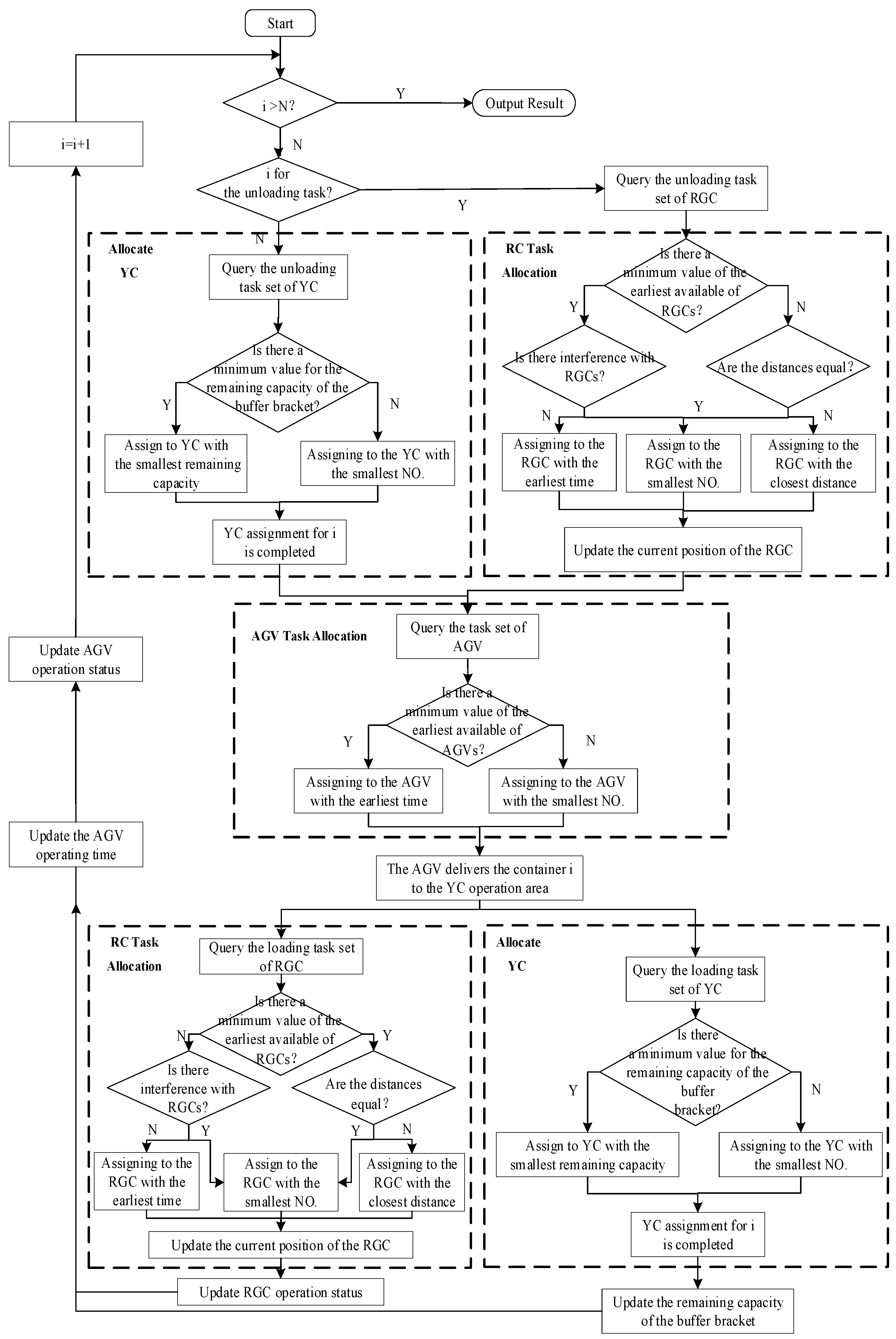
4. Self-Adaptive Chaotic Genetic Algorithm

Heuristic algorithms are widely used in the field of terminal equipment scheduling [45]. Genetic algorithms have a stable mathematical model and theoretical foundation. Studies have shown that fixed crossover and mutation probability fail to maintain the diversity of populations and the convergence of genetic algorithms [4,46]. Adaptive strategies can broaden the search range of genetic algorithms by dynamically adjusting crossover and variation operators (Bao et al. [47]). Furthermore, chaotic motion, being stochastic and ergodic, can help genetic algorithms to escape local optimal solutions [48,49]. Chaos optimization involves mapping chaotic variables to the problem state space and transforming the search process for optimal solutions into the traversal process of chaotic trajectories; thus it prevents the algorithm from getting stuck in local minima [50,51,52].
To enhance the efficiency of algorithmic solutions, we have designed task allocation rules for RGCs, AGVs, and YCs based on the actual operational conditions of a SRACT, as illustrated in Figure 3. Once the loading and unloading sequence of tasks in the chromosome is known, these rules can assist in assigning appropriate devices for each of the following tasks:
RGC task assignment: This involves considering the task attributes of the RGC, including its previous task’s operational status, completion time, location, and quantity. Tasks are assigned sequentially to YC in good condition, starting with the earliest available time, closest proximity to the task, and smallest number. In simultaneous loading and unloading at the same bay, unloading takes priority before loading.
AGV task assignment: The task attributes of the AGV, such as operational status, completion time, and previous tasks, are considered. Tasks are assigned sequentially to AGVs in good condition based on the earliest available time and the smallest number.
YC task assignment: The YC’s task attributes, including its previous task’s completion time, remaining buffer bracket capacity, and number, are considered. Tasks are assigned sequentially to the YC with the earliest available time, largest remaining buffer capacity, and smallest number.
The SCGA for the cooperative scheduling of multiple equipment in the SRACT involves calculating the fitness value of the chromosome population after task assignment according to the abovementioned rules. The adaptive cross-variation probability method is then employed to enhance population diversity during later stages of evolution. Additionally, characteristics of chaotic sequences, such as ergodicity and fuzzy relations, address the genetic algorithm’s limitations in local search ability, enabling it to escape local optimal solutions. The flow of the SCGA is illustrated in Figure 4.

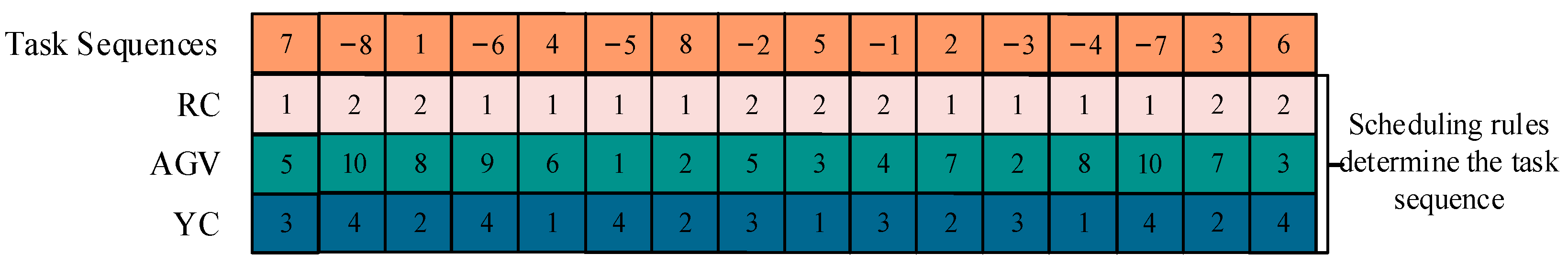
4.1. Encoding and Decoding

This section provides an example using two RGC, ten AGV, and four YC operations, eight unloading containers, and eight loading containers. The first row of the chromosome represents a randomly generated task sequence, with each gene corresponding to a container task. Positive values indicate loading containers, while negative values indicate unloading containers. The second, third, and fourth rows represent RGCs, AGVs, and YCs assigned to perform the tasks based on the assignment mentioned above rules. Since the assignment rules determine the RGC, the AGV, and the YC, the operation sequence must be optimized in subsequent crossover and variation operations. The objective function f aims to minimize the maximum loading and unloading completion time and the total operational energy consumption. The adaptation function is denoted as F ( x i t ) = 1 / f ( x i t ) when x i t represents the i -th individual of the t -th generation. Chromosomes and their operational sequences are presented in Figure 5.

4.2. Select Operation

A binary tournament approach is employed for chromosome selection. This method is easy to implement and prevents falling into local optimum conditions, enabling a more efficient search of the entire solution space. This approach eliminates operation sequences ranked bottom 1/10 of the fitness value directly. Then, two operation sequences are randomly selected for comparison with the remaining ones. The better operation sequence is advanced to the following comparison round, while the worse operation sequence is eliminated. This process continues until the desired population is selected.

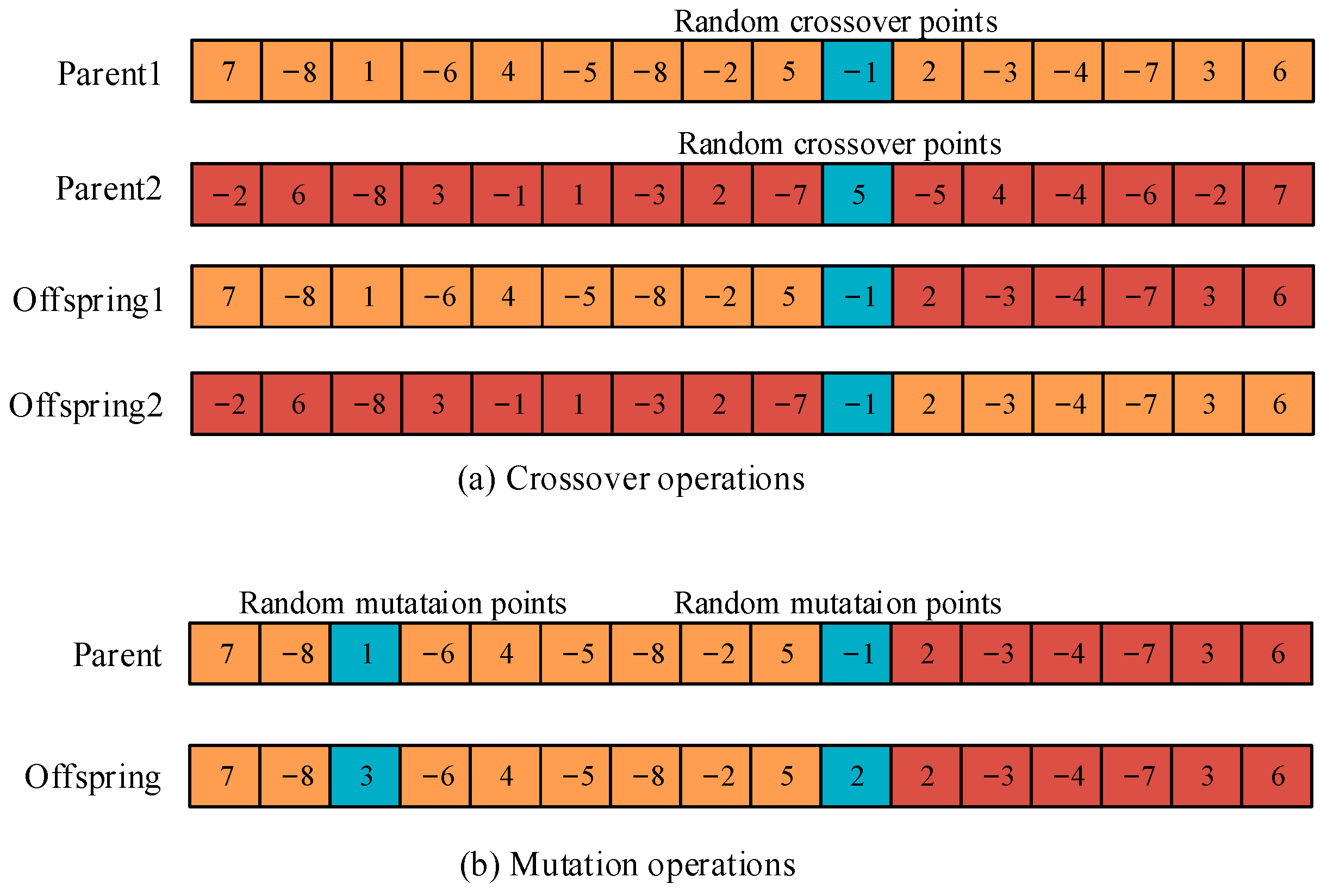
4.3. Crossover and Mutation Operations

In this study, we employed the adaptive strategy that Tang et al. [53] proposed which utilized Equations (50) and (51) to dynamically and nonlinearly adjust the crossover and variation probabilities using trigonometric functions, considering the evolutionary properties of the population. The crossover probability, denoted by p c _ min , p c _ max , and the mutation probability, denoted by p m _ min , p m _ max , are adjusted based on the average fitness value of the population per generation f a v g . The enormous value f between the two loading and unloading task sequences to be crossed and the task sequence’s fitness value f selected for variation are considered. p c and p m represent the crossover and mutation parameters, respectively.
p c = p c + ( p c _ max p c ) · cos ( f a v g f f a v g f c _ min × π 2 ) , f < f a v g p c ( p c p c _ min ) · sin ( f f a v g f c _ max f a v g × π 2 ) , f f a v g
p m = p m + ( p m _ max p m ) · cos ( f a v g f f a v g f m _ min × π 2 ) , f < f a v g p m ( p m p m _ min ) · sin ( f f a v g f m _ max f a v g × π 2 ) , f f a v g
In the genetic operation, a single-point crossover is used for the operation sequences of the selected chromosomes to minimize damage to the chromosome job sequences x i t and to ensure the convergence accuracy of the algorithm. A two-point mutation is employed to improve local random searchability. The specific operations of crossover and mutation are illustrated in Figure 6.

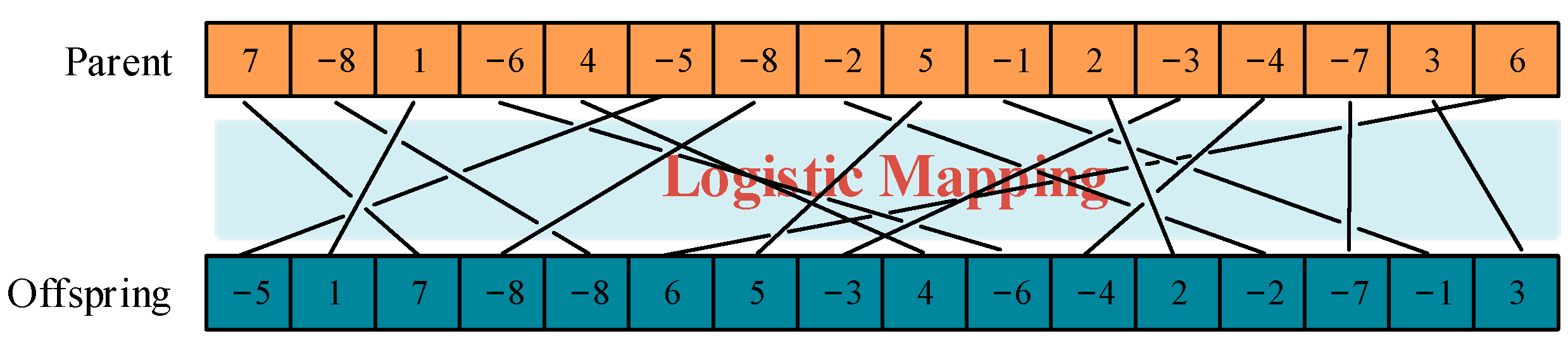
4.4. Chaos Optimization

When the chromosome is iterated multiple times without changing the optimal fitness value, the randomness and ergodicity of chaotic optimization can be leveraged to explore a more optimal solution in the solution space near the original chromosome. This new solution replaces the original one, assisting the genetic algorithm to escape local optimal solutions and achieve overall improvements. This paper selects the commonly used logistic mapping model for chaotic sequences characterized by the following expressions. The control parameter, denoted by α , is crucial in determining the system’s behavior. Notably, when α equals 4, the system reaches a state of complete chaos, so this setting is used in this article.
β n + 1 = α × β n × 1 β n β n 0 , 1 , α 2 , 4
After obtaining the chaotic sequence, the new chromosomes are sorted based on their fitness values. The generated chromosomes with better fitness values replace the old ones, as shown in Figure 7.

4.5. Gene Repair

The operation sequence of the chromosome after cross-variation and chaos optimization may contain duplicated operation tasks. Therefore, checking and correcting the chromosome is necessary by deleting duplicate operation tasks and adding missing operation tasks in sequential order.

4.6. Algorithm Stopping Rules

The algorithm termination guidelines in this paper are as follows: (1) To avoid premature convergence or overfitting, the algorithm stops when the specified number of iterations is reached. (2) If the value of the objective function remains unchanged for n consecutive generations, the further operation becomes computationally wasteful, prompting the algorithm to stop running.

5. Simulation Experiments and Analysis

This study performed three simulation experiments to validate the effectiveness of the proposed model and algorithm. The first experiment verified the effectiveness of the proposed model and algorithm. The second experiment aimed to compare the efficiency of the bi-objective collaborative and single-objective optimization solutions while examining the influence of different weights on the experimental outcomes. The second experiment focused on optimizing the configuration of RGCs, AGVs, and YCs to improve the overall efficiency of the terminal system. Lastly, the fourth experiment investigated the impact of vessel delay duration and container type variation on energy consumption and analyzed the adjustment strategy of AGVs.
The algorithm program was implemented using MATLAB R2018b and executed on a Windows 10 operating system with an i7-12700H processor. The planimetric parameters of the automated sea-rail terminal were configured based on the rail entry model of Terminal J at the Port of Long Beach, USA [7]. The railway loading line consists of three railway tracks, each capable of accommodating a maximum of 40 carriages. The railway operation area also features a temporary storage point for temporary container storage, while the yard is divided into four container areas. Table 1 presents the parameters relevant to loading and unloading equipment in the railway operation area, whereas Table 2 displays the parameters associated with the SCGA.

5.1. Algorithm Validity Verification Experiment

A comparative study was conducted to substantiate the effectiveness of the proposed SCGA, which incorporated scheduling rules for RGCs, AGVs, and YCs. In this study, the algorithm was evaluated against the improved genetic algorithm (IGA), the adaptive adjustment strategy-based genetic algorithm (SGA), and the chaotic genetic algorithm (CGA) proposed by Yue et al. [54]. The comparison experiments were conducted under the configuration scenarios of 120 train–ship tasks, 120 yard–train tasks, 3 RGCs, and 15 AGVs; the bi-objective weights were set as ω 1 = ω 1 = 0.5 for all experiments in this section. Figure 8 illustrated the convergence trends of the four algorithms, providing insights into their performance.
Based on the analysis of Figure 8, it can be observed that the SCGA identified the upper bound solution at iteration 364 as 208.8, the IGA identified the upper bound solution at iteration 427 as 245.1, the SGA identified the upper bound solution at iteration 381 as 239.2, and the CGA identified the upper bound solution at iteration 292 as 223.5. These experimental results highlight the effectiveness of both the adaptive cross-variation probability and the chaotic optimization strategy in overcoming the limitations of the genetic algorithm. The adaptive genetic algorithm also demonstrated superior solution speed compared to the chaotic genetic algorithm. Conversely, the chaotic genetic algorithm exhibited better solution results, indicating its superior local search capability. Moreover, the adaptive adjustment strategy contributed to an accelerated convergence speed of the algorithm. Collectively, these findings further validated the effectiveness of the SCGA proposed in this study.

5.2. Experiment on Comparing Bi-Objective and Single-Objective Optimizatiom

To validate the effectiveness of the bi-objective optimization approach adopted in this study, which considers both efficiency and energy consumption, a total of 13 experiments were conducted in this section. The experiments recorded loading and unloading completion times and operational energy consumption data. Each experiment was repeated 10 times, and the results were averaged. The summarized findings are presented in Table 3. In the table, MCT represents the maximum completion time and OEC represents the operational energy consumption of the RGCs and AGVs. N/R/V denotes the number of containers, RGCs and AGVs, respectively. Furthermore, the bi-objective weights were set as for all experiments in this section.
The results have demonstrated that the bi-objective model outperforms the single-objective model in terms of both the maximum completion time of RGCs and the total operational energy consumption of both the RGCs and the AGVs. Specifically, the bi-objective model achieved a significant 7.74% reduction in operational energy consumption compared to the single objective of minimizing the maximum loading and unloading completion time. Additionally, the maximum loading and unloading completion time was reduced by 4.06% in the bi-objective model compared to the single objective of considering only the total operational energy consumption. These findings provide strong evidence for the effectiveness of the proposed bi-objective optimization model in achieving synergistic optimization of both the loading and unloading operational efficiency and the operational energy consumption of the equipment.

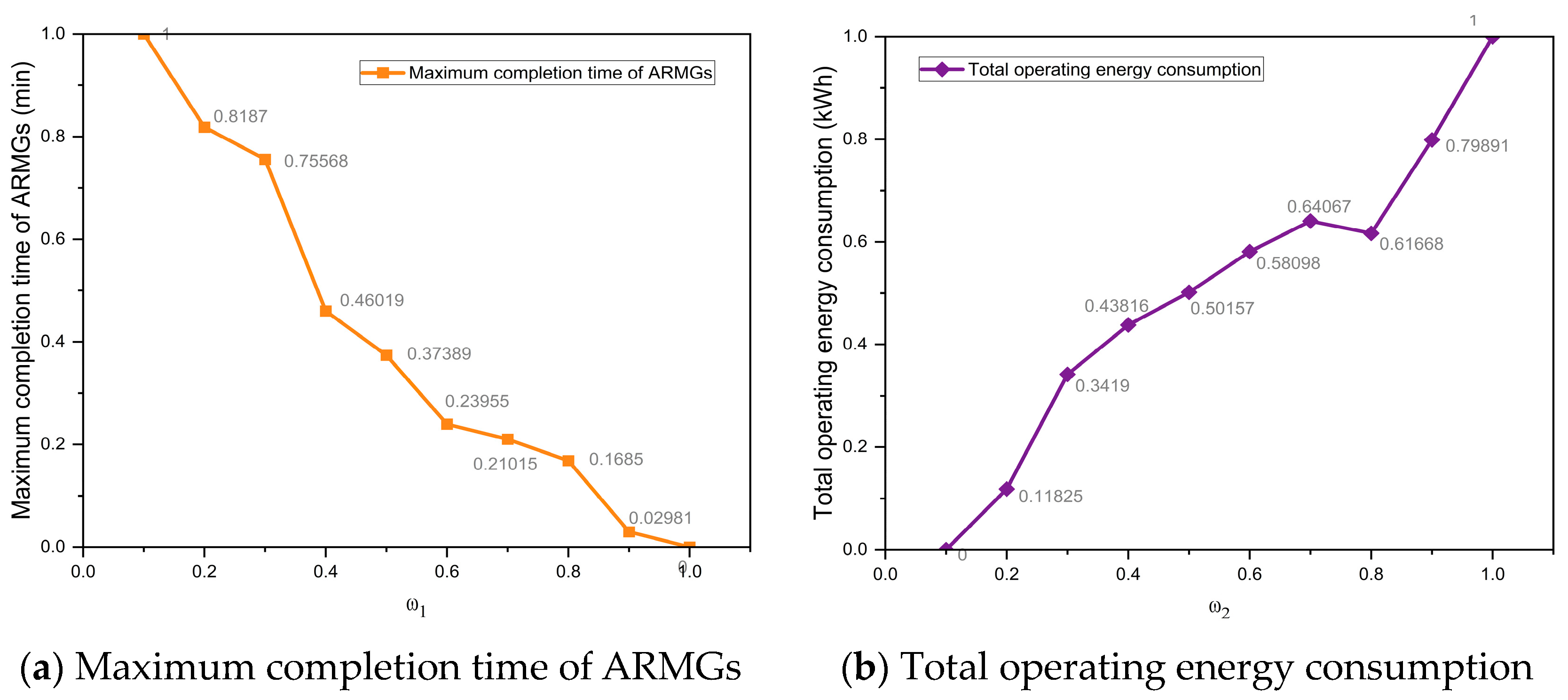
5.3. Normalization and the Impact of Weights

Because the maximum completion time and operating energy consumption are variables of different units, they need to be normalized. The normalized maximum completion time ( N M C T ) and the normalized operational energy consumption ( N O E C ) will handle as follows:
N M C T = M C T min ( M C T ) max ( M C T ) min ( M C T )
N O E C = O E C min ( O E C ) max ( O E C ) min ( O E C )
We consider the operation of 3 RGCs and 12 AGVs for 120 train–ship tasks and 120 yard–train tasks to further investigate the impact of weight values on efficiency and energy consumption objectives. After normalized data processing, the experimental results are depicted in Figure 9. As shown in Figure 9a, an increase in the efficiency weight leads to a gradual reduction in the completion time of loading and unloading operations. This indicates that assigning a higher weight to efficiency results in shorter task completion times for container operations. Conversely, Figure 9b reveals that the total operational energy consumption of both RGCs and AGVs increases as the efficiency weight increases. It is worth noting that when the total completion time and energy consumption reach a relatively low level, this finding aligns with the conclusions of previous research [55]. Consequently, this weight value is consistently utilized in the objective function throughout subsequent studies, ensuring the system’s overall effectiveness.

5.4. Optimization of RGCs, AGVs, and YCs Configurations Experiments

In the scenario where three trains simultaneously enter the port, with each train consisting of 40 carriages and the ships arriving on time, a total of 120 train–ship tasks and 120 yard–train tasks are generated. In the Table 4, the variables R/V represent the RGC and AGV numbers, respectively. The normalized upper bound solution ( N U B S ) is the normalized and weighted objective function value of time and energy consumption. In this subsection, 39 experiments were conducted, each repeated 10 times, and the results averaged. The simulation results are presented in Table 4.
As indicated in Table 4, the optimal configuration for minimizing the collaborative value of completion time for loading and unloading operations and total operational energy consumption relies on the number of RGCs and AGVs deployed. For the case of two RGCs, the optimal configuration involves deploying ten AGVs. This configuration yields a maximum RGC completion time of 219.23 min and a total operational energy consumption of 423.14 kWh, and the N U B S is 0.419. By increasing the number of RGCs to 3 and AGVs to 15, the completion time of the loading and unloading operation decreases to 114.26 min, along with a reduction in the total operational energy consumption to 350.38 kWh, while the N U B S is 0.005. Moreover, further improvement is achieved by deploying 4 RGCs and 20 AGVs, resulting in a collaborative value reduction in the maximum completion time for the RGC to 152.75 min and a decrease in the total operational energy consumption to 375.56 kWh, while the N U B S is 0.154. Consequently, the optimal configuration ratio of RGCs to AGVs, attaining the lowest collaborative value, is determined to be 1:5.
The configuration of 3 RGCs and 15 AGVs achieved the lowest value of bi-objective co-optimization, as shown in Table 4. Additionally, Table 5 provided details of the tasks and operation order of the AGVs.
Through an analysis of the data presented in Table 5, the operational sequence for the 15 AGVs can be established. AGV No. 1 is designated to initiate the unloading task for container one, followed by the loading task for Container 8, and subsequently, the unloading task for Container 16, continuing similarly. By adhering to this predetermined sequence, effective scheduling and coordination of the assigned tasks for the 15 AGVs are achieved, thereby facilitating an optimized logistics operation.

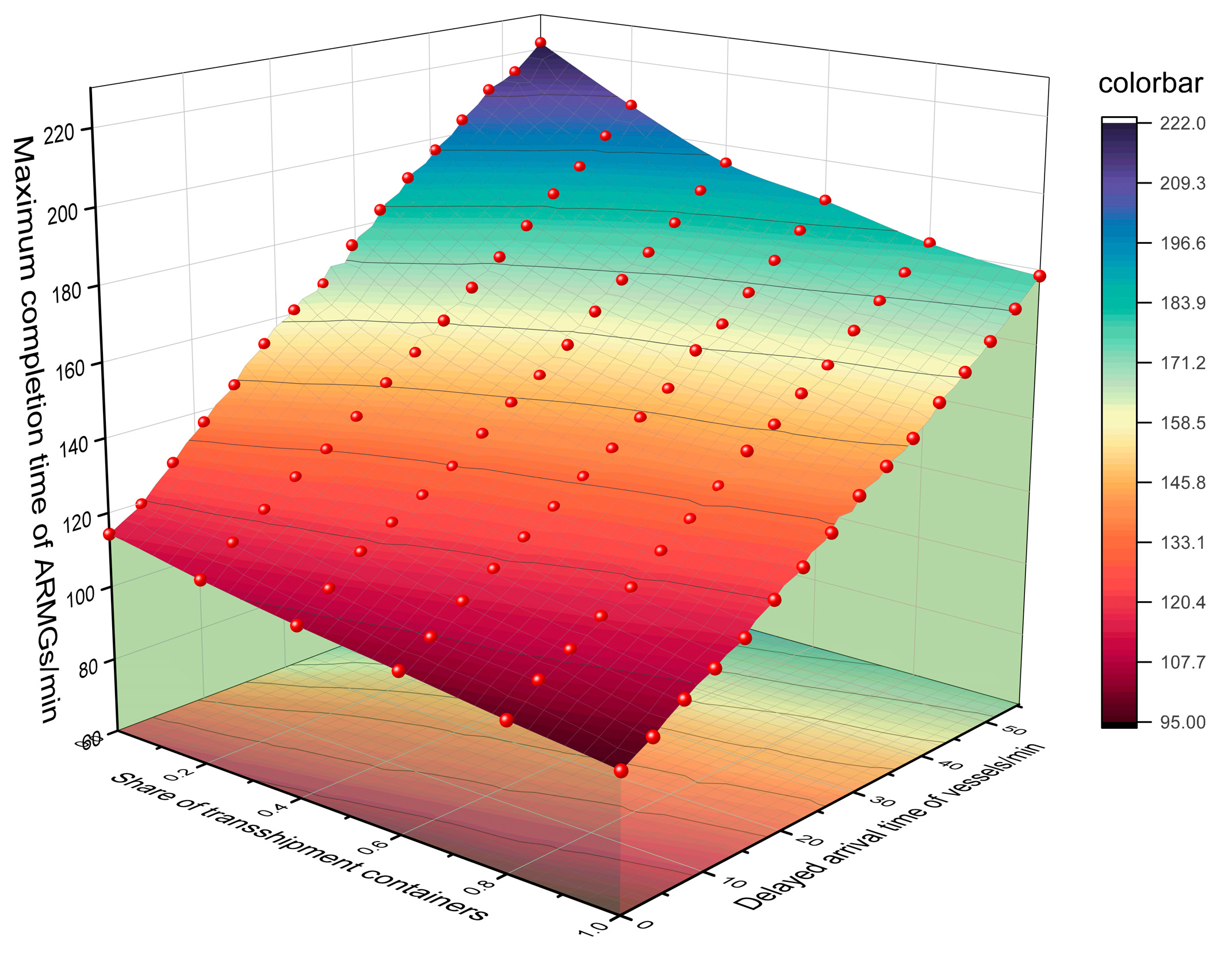
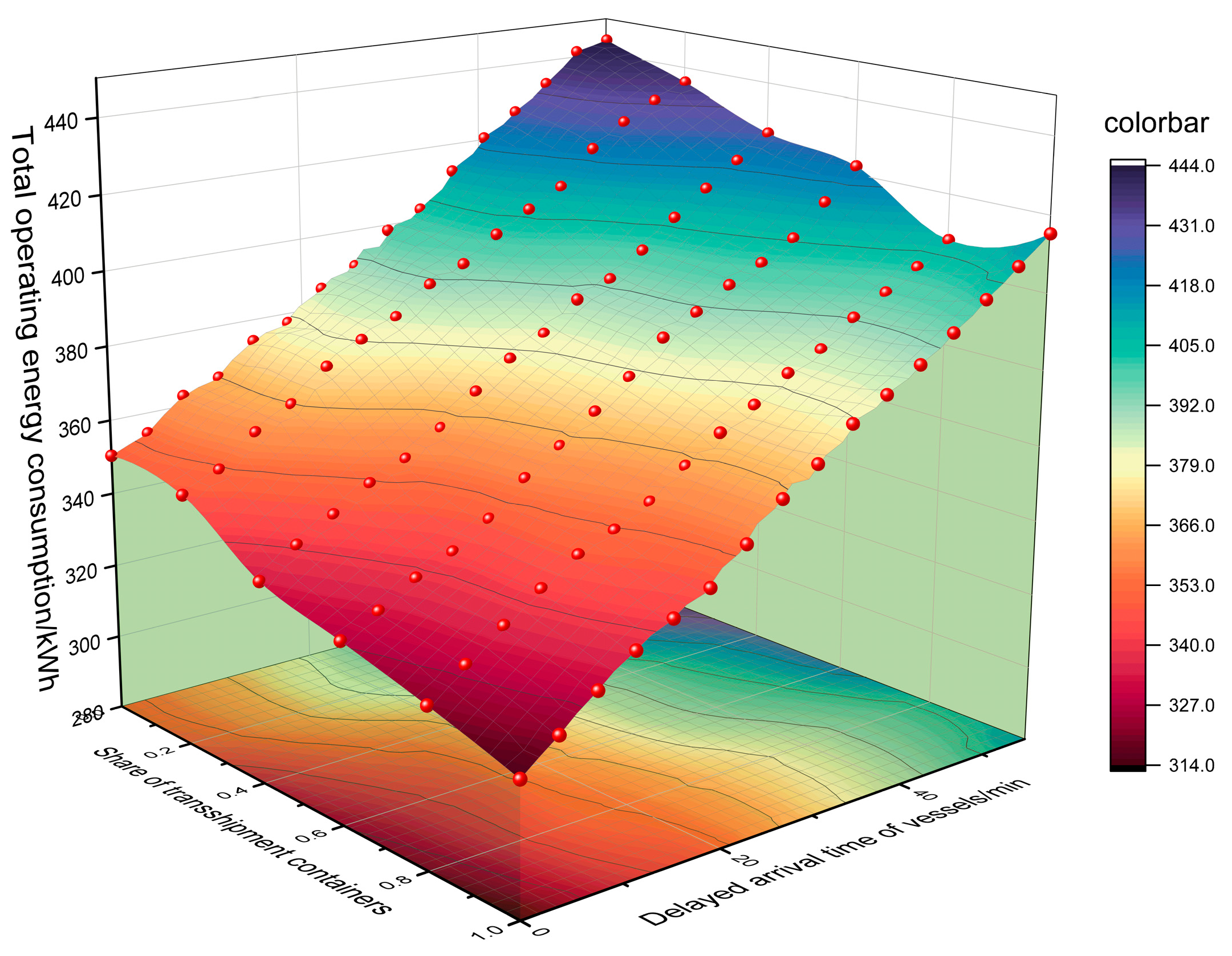
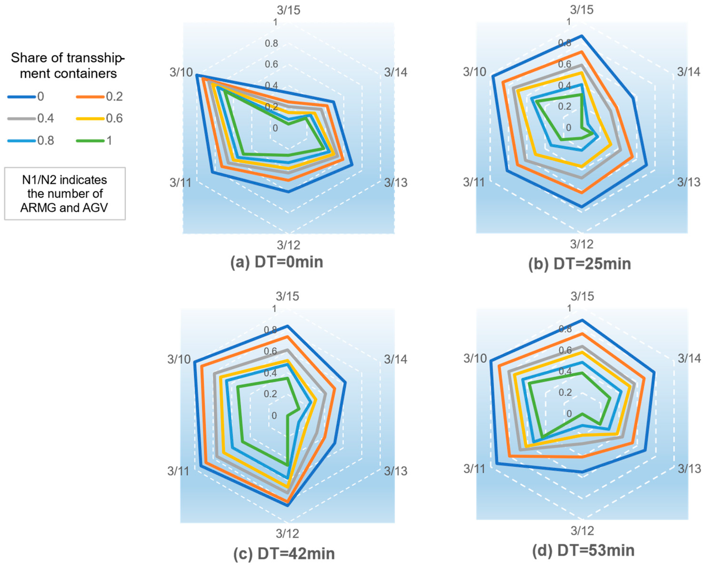
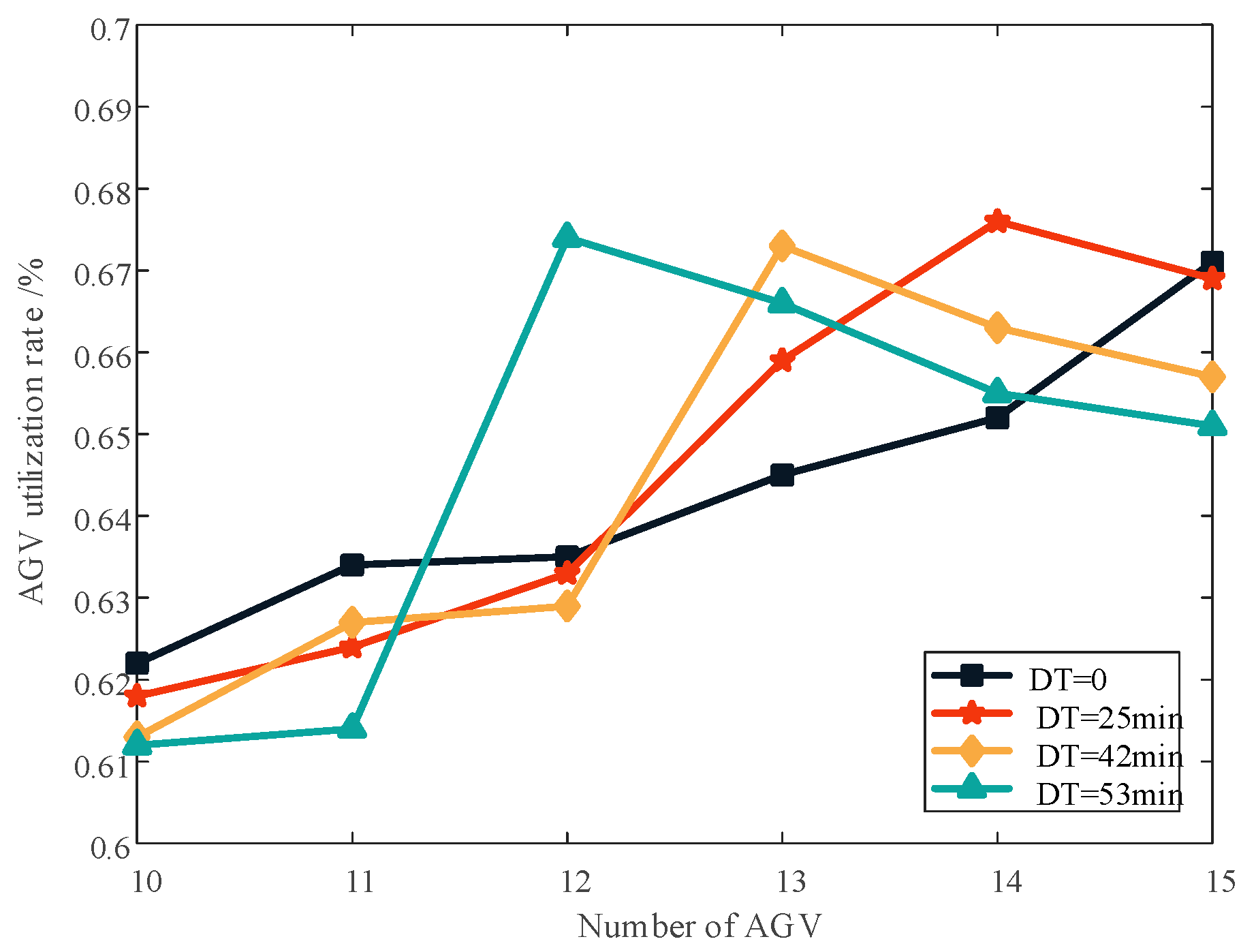
5.5. Impact of Vessel Delays and Container Type Change

Uncertainties from various factors, such as weather conditions and port traffic, can influence the arrival times of ships. Moreover, the number and composition of containers on a train are subject to change. In this section, the effects of different ship delay arrival times and container types on the completion time and total energy consumption of loading and unloading operations are studied, as visually illustrated in Figure 10 and Figure 11.
As depicted in Figure 10 and Figure 11, there exists a positive relationship between the delayed arrival time of vessels and both the completion time of loading and unloading operations and the total operational energy consumption. Conversely, an inverse relationship is observed between the proportion of train–yard tasks and these performance indicators. Specifically, on the one hand, as the delayed arrival time of ships increases, the completion time of loading and unloading operations, as well as the total operational energy consumption, also increases. On the other hand, increasing the proportion of train–yard tasks can effectively alleviate the operational pressure on the RGC, thereby reducing the completion time of loading and unloading operations and the total operational energy consumption. These findings highlight the significance of considering vessel delays and optimizing the task allocation strategy to enhance operational efficiency and minimize energy consumption.
In the event of a delayed ship arrival, AGVs that would have been assigned to the operate train–ship task may instead be allocated to the RGC for the operate train–yard task, using the same equipment quantity configuration as if the ship had arrived on time. However, this allocation adjustment can lead to increased waiting time for AGVs at the RGC, ultimately impacting the completion time of loading and unloading operations and the total operational energy consumption of the equipment. We dynamically adjusted the number of AGVs for different delayed vessel arrival times to investigate these effects. We observed the corresponding changes on N U B S . The experimental results are presented in Figure 12.
Figure 12 demonstrates that a moderate reduction in AGVs can effectively reduce costs when ship delays are short. Conversely, maintaining the RGC to AGV ratio of 1:4 for longer vessel delays achieves upper bound solutions in terms of the objective function, which encompasses the synergistic optimization of loading and unloading completion time and total operational energy consumption. Specifically, with the RGCs, configuring 12 AGVs instead of 15 AGVs can reduce loading and unloading completion time by 5.16% and total operational energy consumption by 8.56%. However, continuous reduction in AGVs may lead to increased efficiency and energy consumption.
Figure 13 displays the AGV utilization rates in different experiments under various AGV quantity configurations. As observed from the figure, adjusting the number of AGVs can increase their utilization without altering the RGC configurations. Specifically, when a ship arrives without delay, the AGV utilization rate stands at 67.1%. When the ship’s arrival is delayed by 25 min, maintaining the original configuration will cause a 2% decrease in AGV utilization. At this point, reducing the number of AGVs to 14 could increase the utilization by 7%. If the ship’s arrival is delayed by 42 min, continuing with 14 AGVs will lead to a 13% drop in utilization. Reducing the AGVs to 13 in this case could increase utilization by 14%. When the ship is delayed by 53 min, continuing with 13 AGVs will cause a 7% decline in utilization, but reducing the AGV count to 12 could increase the utilization by 8%. However, it is worth noting that continuously reducing the number of AGVs will not enhance their utilization. The minimum AGV configuration is 12. If the number of AGVs falls below this, the utilization rate will drastically decline.
In general, when there is a delay in the arrival of a ship at the port, maintaining a constant number of AGVs leads to an increase in the completion time and total operational energy consumption of the loading and unloading operation and a decrease in AGV utilization. Therefore, in practical scheduling, monitoring ship arrivals and making necessary adjustments to the AGV allocation is crucial. By adjusting the rail crane to an AGV ratio from 1:5 to 1:4, the utilization of AGVs can be increased by 23% when a ship’s arrival is delayed beyond a specific time.

6. Conclusions

This paper addresses the collaborative equipment scheduling issues in a sea-rail intermodal automated container terminal. It introduces six container flow directions and seven AGV flow directions during train loading and unloading in the terminal. Considering the collaboration between efficiency and energy consumption, a bi-objective collaboration optimization model is proposed for minimizing loading and unloading completion time and total energy consumption of RC and AGV operations. The model is solved using an adaptive chaotic genetic algorithm based on the task assignment scheduling rules of the sea-rail automated container terminal. A multi-equipment collaborative scheduling scheme that considers efficiency and energy consumption is obtained. The experimental results demonstrate that the bi-objective collaborative optimization model outperforms the single-objective model. The above simulation experiments prove the following: (1) Compared to the single-objective model, the bi-objective optimization model proposed in this study can achieve a 4.06% reduction in the completion time of loading and unloading operations and a 7.74% reduction in the energy consumption of equipment operations. (2) The SCGA algorithm used in this research converges faster and yields superior solutions compared to other heuristic algorithms. (3) When all the containers on the train are allocated for rail transport, the optimal configuration of RCs to AGVs is 1:5. (4) Adjusting the number of AGVs during the delayed arrival of ships can effectively shorten the maximum completion time of RCs, reduce total operational energy consumption, and enhance the utilization rate of AGVs.
However, there are still limitations in this study. First, future research directions of this work should further consider the impact of more complex operational conditions on equipment scheduling. Secondly, the current study is only conducted under the specific layout shown in Figure 1; further research is needed for other layouts of sea-rail automated container terminals. Thirdly, how to systematically compare heuristic algorithms with exact algorithms in the port equipment scheduling environment to obtain optimal solutions is also an important task for future work. Lastly, active collaborations with real-world terminals should be sought to test and validate the models and algorithms in real operational environments.

Author Contributions

Conceptualization, supervision, funding acquisition, project administration, methodology, Y.Y.; writing—original draft, software, S.S.; writing—review and editing, S.H.; validation, formal analysis, simulated cases, Y.J.; validation, resources, data provision, H.Y.; verification, corrections, experiment supervision, X.W.; visualization, J.Z. All authors have read and agreed to the published version of the manuscript.

Funding

This work was supported by the Shanghai Association for Science and Technology (Grant No. 18295801100).

Data Availability Statement

The data used to support the findings of this study are included within the article.

Conflicts of Interest

The authors declare no conflict of interest.

References

  1. Millefiori, L.M.; Braca, P.; Zissis, D.; Spiliopoulos, G.; Marano, S.; Willett, P.K.; Carniel, S. COVID-19 impact on global maritime mobility. Sci. Rep. 2021, 11, 18039. [Google Scholar] [CrossRef]
  2. Yang, Y.; Zhong, M.; Dessouky, Y.; Postolache, O. An integrated scheduling method for AGV routing in automated container terminals. Comput. Ind. Eng. 2018, 126, 482–493. [Google Scholar] [CrossRef]
  3. Yu, H.; Huang, M.; He, J.; Tan, C. The clustering strategy for stacks allocation in automated container terminals. Marit. Policy Manag. 2022, 1–16. [Google Scholar] [CrossRef]
  4. Chang, Y.; Zhu, X.; Haghani, A. Modeling and solution of joint storage space allocation and handling operation for outbound containers in rail-water intermodal container terminals. IEEE Access 2019, 7, 55142–55158. [Google Scholar] [CrossRef]
  5. Reis, V.; Meier, J.F.; Pace, G.; Palacin, R. Rail and multi-modal transport. Res. Transp. Econ. 2013, 41, 17–30. [Google Scholar] [CrossRef]
  6. Boysen, N.; Fliedner, M.; Jaehn, F.; Pesch, E. A survey on container processing in railway yards. Transp. Sci. 2013, 47, 312–329. [Google Scholar] [CrossRef]
  7. Yang, Y.; He, S.; Sun, S. Research on the Cooperative Scheduling of ARMGs and AGVs in a Sea–Rail Automated Container Terminal under the Rail-in-Port Model. J. Mar. Sci. Eng. 2023, 11, 557. [Google Scholar] [CrossRef]
  8. Li, J.; Yan, L.; Xu, B. Research on Multi-Equipment Cluster Scheduling of U-Shaped Automated Terminal Yard and Railway Yard. J. Mar. Sci. Eng. 2023, 11, 417. [Google Scholar] [CrossRef]
  9. Wang, L.; Zhu, X. Rail mounted gantry crane scheduling optimization in railway container terminal based on hybrid handling mode. Comput. Intell. Neurosci. 2014, 2014, 682486. [Google Scholar] [CrossRef]
  10. Li, W.; Du, S.; Zhong, L.; He, L. Multiobjective Scheduling for Cooperative Operation of Multiple Gantry Cranes in Railway Area of Container Terminal. IEEE Access 2022, 10, 46772–46781. [Google Scholar] [CrossRef]
  11. Fu, X.; Yang, Y. Modeling and analyzing cascading failures for Internet of Things. Inf. Sci. 2021, 545, 753–770. [Google Scholar] [CrossRef]
  12. Fu, X.; Yang, Y. Analysis on invulnerability of wireless sensor networks based on cellular automata. Reliab. Eng. Syst. Saf. 2021, 212, 107616. [Google Scholar] [CrossRef]
  13. Fu, X.; Li, Q.; Li, W. Modeling and analysis of industrial IoT reliability to cascade failures: An information-service coupling perspective. Reliab. Eng. Syst. Saf. 2023, 239, 109517. [Google Scholar] [CrossRef]
  14. Chen, X.; Wu, S.; Shi, C.; Huang, Y.; Yang, Y.; Ke, R.; Zhao, J. Sensing Data Supported Traffic Flow Prediction via Denoising Schemes and ANN: A Comparison. IEEE Sens. J. 2020, 20, 14317–14328. [Google Scholar] [CrossRef]
  15. Iris, Ç.; Christensen, J.; Pacino, D.; Ropke, S. Flexible ship loading problem with transfer vehicle assignment and scheduling. Transp. Res. Part B Methodol. 2018, 111, 113–134. [Google Scholar] [CrossRef]
  16. Zhou, C.; Zhu, S.; Bell, M.G.H.; Lee, L.H.; Chew, E.P. Emerging technology and management research in the container terminals: Trends and the COVID-19 pandemic impacts. Ocean Coast. Manag. 2022, 230, 106318. [Google Scholar] [CrossRef]
  17. Iris, Ç.; Lam, J.S.L. A review of energy efficiency in ports: Operational strategies, technologies and energy management systems. Renew. Sustain. Energy Rev. 2019, 112, 170–182. [Google Scholar] [CrossRef]
  18. Wu, Y.; Li, W.; Petering, M.E.H.; Goh, M.; de Souza, R. Scheduling multiple yard cranes with crane interference and safety distance requirement. Transp. Sci. 2015, 49, 990–1005. [Google Scholar] [CrossRef]
  19. Chu, F.; He, J.; Zheng, F.; Liu, M. Scheduling multiple yard cranes in two adjacent container blocks with position-dependent processing times. Comput. Ind. Eng. 2019, 136, 355–365. [Google Scholar] [CrossRef]
  20. Sha, M.; Zhang, T.; Lan, Y.; Zhou, X.; Qin, T.; Yu, D.; Chen, K. Scheduling optimization of yard cranes with minimal energy consumption at container terminals. Comput. Ind. Eng. 2017, 113, 704–713. [Google Scholar] [CrossRef]
  21. Chen, X.; Wang, Z.; Hua, Q.; Shang, W.-L.; Luo, Q.; Yu, K. AI-Empowered Speed Extraction via Port-Like Videos for Vehicular Trajectory Analysis. IEEE Trans. Intell. Transp. Syst. 2023, 24, 4541–4552. [Google Scholar] [CrossRef]
  22. Zhong, M.; Yang, Y.; Dessouky, Y.; Postolache, O. Multi-AGV scheduling for conflict-free path planning in automated container terminals. Comput. Ind. Eng. 2020, 142, 106371. [Google Scholar] [CrossRef]
  23. Hu, H.; Yang, X.; Xiao, S.; Wang, F. Anti-conflict AGV path planning in automated container terminals based on multi-agent reinforcement learning. Int. J. Prod. Res. 2023, 61, 65–80. [Google Scholar] [CrossRef]
  24. Kim, K.H.; Lee, K.M.; Hwang, H. Sequencing delivery and receiving operations for yard cranes in port container terminals. Int. J. Prod. Econ. 2003, 84, 283–292. [Google Scholar] [CrossRef]
  25. Lee, B.K.; Kim, K.H. Comparison and evaluation of various cycle-time models for yard cranes in container terminals. Int. J. Prod. Econ. 2010, 126, 350–360. [Google Scholar] [CrossRef]
  26. Liu, W.; Zhu, X.; Wang, L.; Li, S. Rolling horizon based robust optimization method of quayside operations in maritime container ports. Ocean Eng. 2022, 256, 111505. [Google Scholar] [CrossRef]
  27. Zheng, F.; Man, X.; Chu, F.; Liu, M.; Chu, C. Two yard crane scheduling with dynamic processing time and interference. IEEE Trans. Intell. Transp. Syst. 2018, 19, 3775–3784. [Google Scholar] [CrossRef]
  28. Nossack, J.; Briskorn, D.; Pesch, E. Container dispatching and conflict-free yard crane routing in an automated container terminal. Transp. Sci. 2018, 52, 1059–1076. [Google Scholar] [CrossRef]
  29. Eilken, A. A decomposition-based approach to the scheduling of identical automated yard cranes at container terminals. J. Sched. 2019, 22, 517–541. [Google Scholar] [CrossRef]
  30. Lu, H.; Wang, S. A study on multi-ASC scheduling method of automated container terminals based on graph theory. Comput. Ind. Eng. 2019, 129, 404–416. [Google Scholar] [CrossRef]
  31. Zhang, Q.; Hu, W.; Duan, J.; Qin, J. Cooperative Scheduling of AGV and ASC in Automation Container Terminal Relay Operation Mode. Math. Probl. Eng. 2021, 2021, 5764012. [Google Scholar] [CrossRef]
  32. Yang, X.-M.; Jiang, X.-J. Yard Crane Scheduling in the Ground Trolley-Based Automated Container Terminal. Asia-Pac. J. Oper. Res. 2020, 37, 2050007. [Google Scholar] [CrossRef]
  33. Chen, X.; He, S.; Zhang, Y.; Tong, L.; Shang, P.; Zhou, X. Yard crane and AGV scheduling in automated container terminal: A multi-robot task allocation framework. Transp. Res. Part C Emerg. Technol. 2020, 114, 241–271. [Google Scholar] [CrossRef]
  34. Hsu, H.-P.; Tai, H.-H.; Wang, C.-N.; Chou, C.-C. Scheduling of collaborative operations of yard cranes and yard trucks for export containers using hybrid approaches. Adv. Eng. Inform. 2021, 48, 101292. [Google Scholar] [CrossRef]
  35. Zhou, C.; Lee, B.K.; Li, H. Integrated optimization on yard crane scheduling and vehicle positioning at container yards. Transp. Res. E Logist. Transp. Rev. 2020, 138, 101966. [Google Scholar] [CrossRef]
  36. Peng, Y.; Wang, W.; Liu, K.; Li, X.; Tian, Q. The impact of the allocation of facilities on reducing carbon emissions from a green container terminal perspective. Sustainability 2018, 10, 1813. [Google Scholar] [CrossRef]
  37. Li, X.; Peng, Y.; Huang, J.; Wang, W.; Song, X. Simulation study on terminal layout in automated container terminals from efficiency, economic and environment perspectives. Ocean Coast. Manag. 2021, 213, 105882. [Google Scholar] [CrossRef]
  38. Zhao, Q.; Ji, S.; Zhao, W.; De, X. A Multilayer Genetic Algorithm for Automated Guided Vehicles and Dual Automated Yard Cranes Coordinated Scheduling. Math. Probl. Eng. 2020, 2020, 5637874. [Google Scholar] [CrossRef]
  39. Iris, Ç.; Lam, J.S.L. Optimal energy management and operations planning in seaports with smart grid while harnessing renewable energy under uncertainty. Omega 2021, 103, 102445. [Google Scholar] [CrossRef]
  40. Ballis, A.; Golias, J. Comparative evaluation of existing and innovative rail–road freight transport terminals. Transp. Res. Part A Policy Pract. 2002, 36, 593–611. [Google Scholar] [CrossRef]
  41. Li, X.; Otto, A.; Pesch, E. Solving the single crane scheduling problem at rail transshipment yards. Discret. Appl. Math. 2018, 264, 134–147. [Google Scholar] [CrossRef]
  42. Ren, G.; Wang, X.; Cai, J.; Guo, S. Allocation and scheduling of handling resources in the railway container terminal based on crossing crane area. Sustainability 2021, 13, 1190. [Google Scholar] [CrossRef]
  43. Yan, B.; Zhu, X.; Wang, L.; Chang, Y. Integrated Scheduling of Rail-Mounted Gantry Cranes, Internal Trucks and Reach Stackers in Railway Operation Area of Container Terminal. Transp. Res. Rec. 2018, 2672, 47–58. [Google Scholar] [CrossRef]
  44. Chang, Y.; Zhu, X.; Yan, B.; Wang, L. Integrated scheduling of handling operations in railway container terminals. Transp. Lett. 2019, 11, 402–412. [Google Scholar] [CrossRef]
  45. Iris, Ç.; Pacino, D.; Ropke, S. Improved formulations and an Adaptive Large Neighborhood Search heuristic for the integrated berth allocation and quay crane assignment problem. Transp. Res. E Logist. Transp. Rev. 2017, 105, 123–147. [Google Scholar] [CrossRef]
  46. El Aziz, M.A.; Ewees, A.A.; Hassanien, A.E. Multi-objective whale optimization algorithm for content-based image retrieval. Multimed. Tools Appl. 2018, 77, 26135–26172. [Google Scholar] [CrossRef]
  47. Bao, X.; Xiong, Z.; Zhang, N.; Qian, J.; Wu, B.; Zhang, W. Path-oriented test cases generation based adaptive genetic algorithm. PLoS ONE 2017, 12, e0187471. [Google Scholar] [CrossRef]
  48. Zheng, Y.; Li, Y.; Wang, G.; Chen, Y.; Xu, Q.; Fan, J.; Cui, X. A Novel Hybrid Algorithm for Feature Selection Based on Whale Optimization Algorithm. IEEE Access 2019, 7, 14908–14923. [Google Scholar] [CrossRef]
  49. Dehkordi, A.A.; Sadiq, A.S.; Mirjalili, S.; Ghafoor, K.Z. Nonlinear-based Chaotic Harris Hawks Optimizer: Algorithm and Internet of Vehicles application. Appl. Soft Comput. 2021, 109, 107574. [Google Scholar] [CrossRef]
  50. Ali, T.S.; Ali, R. A new chaos based color image encryption algorithm using permutation substitution and Boolean operation. Multimed. Tools Appl. 2020, 79, 19853–19873. [Google Scholar] [CrossRef]
  51. An, F.-P.; Liu, J.-E. Image Encryption Algorithm Based on Adaptive Wavelet Chaos. J. Sens. 2019, 2019, 2768121. [Google Scholar] [CrossRef]
  52. Zhang, L.; Zhang, X. Multiple-image encryption algorithm based on bit planes and chaos. Multimed. Tools Appl. 2020, 79, 20753–20771. [Google Scholar] [CrossRef]
  53. Tang, L.; Zhao, J.; Liu, J. Modeling and solution of the joint quay crane and truck scheduling problem. Eur. J. Oper. Res. 2014, 236, 978–990. [Google Scholar] [CrossRef]
  54. Yue, L.; Fan, H.; Zhai, C. Joint configuration and scheduling optimization of a dual-trolley quay crane and Automatic guided vehicles with consideration of vessel stability. Sustainability 2020, 12, 24. [Google Scholar] [CrossRef]
  55. Peng, H.; Wen, W.-S.; Tseng, M.-L.; Li, L.-L. Joint optimization method for task scheduling time and energy consumption in mobile cloud computing environment. Appl. Soft Comput. 2019, 80, 534–545. [Google Scholar] [CrossRef]
Figure 1. Layout for the SRACT.
Jmse 11 01975 g001
Figure 2. Operation cycle diagram of the SRACT under the loading and unloading mode.
Jmse 11 01975 g002
Figure 3. Task allocation process of the RGC, AGV, and YC.
Jmse 11 01975 g003
Figure 4. Flowchart of SCGA based on allocation rule.
Jmse 11 01975 g004
Figure 5. Schematic diagram of chromosomes and their operational sequences.
Jmse 11 01975 g005
Figure 6. Crossover and mutation operations.
Jmse 11 01975 g006
Figure 7. Chaotic optimization.
Jmse 11 01975 g007
Figure 8. Comparison of iterative curves between the SCGA and other algorithms.
Jmse 11 01975 g008
Figure 9. Changes in efficiency and energy consumption with weights.
Jmse 11 01975 g009
Figure 10. The effect of vessel delays and the train–yard task ratio on the maximum completion time of RGCs.
Jmse 11 01975 g010
Figure 11. Impact of vessel delays and the train–yard task ratio on total operational energy consumption.
Jmse 11 01975 g011
Figure 12. Effect of ship delay time (DT) and share of transshipment containers on NUBS.
Jmse 11 01975 g012
Figure 13. Variations in the utilization rate by adjusting AGV configuration for different vessel delays.
Jmse 11 01975 g013
Table 1. ACT parameters.
ParametersNumerical Values
Elevation height for the RGC10 m
Container widths2.5 m
Distance between carriages17 m
Railway loading and unloading line spacing2.5 m
Traveling speed of the RGC gantry80 m/min
Traveling speed of the RGC spreader85 m/min
Average handling time for a task by YC1.5 min
Buffer capacity of the yard4TEU
Energy consumption of one RGC gantry during operation30 kWh/h
Energy consumption of one RGC spreader during motion20 kWh/h
Waiting energy consumption of one RGC15 kWh/h
Energy consumption of one AGV with container21 kWh/h
Energy consumption of one AGV without container14 kWh/h
Safety distance between two RGCs1 carriage
Waiting energy consumption of one AGV9 kWh/h
Travel speed of the AGV with container210 m/min
Travel speed of the AGV without container350 m/min
Table 2. Parameters of the SCGA.
ParametersValueParametersValue
Population size100Maximum Iterations500
Crossover probability[0.4, 0.9]Mutation probability[0.01, 0.1]
Crossover parameters0.6Mutation parameters0.05
Table 3. Comparison of bi-objective collaboration and single-objective optimization solutions.
No.N/R/VBi-ObjectiveSingle-ObjectiveGap1Gap2
MCT/minOEC/kWhMCT/minOEC/kWhMCT (%)OEC (%)
MaxMinMeanMaxMinMean
110/3/421.816.918.434.628.430.120.834.911.713.8
210/3/618.412.914.525.721.522.917.027.914.918.0
315/3/435.631.231.548.744.445.232.250.42.010.3
415/3/625.721.524.240.736.337.125.740.86.29.2
520/3/439.738.038.862.361.862.039.063.20.52.0
620/3/633.929.932.752.249.150.532.853.10.24.9
730/3/657.049.852.587.984.584.753.692.92.18.8
830/3/851.546.747.985.879.981.348.490.71.010.4
940/3/661.658.960.8101.396.497.564.7105.46.17.5
1040/3/858.553.355.795.191.591.656.699.21.77.7
1150/3/881.280.080.3137.9134.5135.483.6137.94.01.8
1250/3/1082.977.078.2136.3132.4132.978.7137.90.63.6
13100/3/10136.8132.8135.6314.8308.7310.4138.2318.71.82.6
Table 4. Results for the different device configurations.
No.R/VMCT OEC N U B S CPU/sNo.R/VMCT OEC N U B S CPU/s
12/4348.03549.361.000 194.5213/17135.88363.570.086 197.3
22/5322.56538.420.913 195.4223/18137.24379.020.121 196.4
32/6287.93465.980.680 190.4234/8224.05484.840.554 193.4
42/7257.83444.10.559 191.0244/9210.17471.170.491 190.2
52/8241.07393.560.416 192.7254/10193.7454.720.416 189.6
62/9222.4408.830.398 193.2264/11187.36418.670.328 201.2
72/10219.23423.140.419 192.3274/12184.85403.190.291 192.1
82/11221.4432.980.444 193.9284/13176.48390.340.244 203.0
92/12222.75438.360.458 194.6294/14171.64378.710.208 194.3
103/6213.82428.320.415 190.4304/15167.29367.140.174 194.8
113/7198.71407.120.334 199.0314/16166.07366.750.170 195.4
123/8188.47398.810.291 203.7324/17163.68368.510.168 197.7
133/9174.08386.140.229 197.1334/18160.1369.010.159 193.8
143/10162.74372.510.173 202.8344/19156.39372.670.157 195.2
153/11153.4363.570.131 198.3354/20152.75375.560.154 196.8
163/12144.09348.020.077 193.2364/21153.68386.180.177 196.4
173/13144.6357.330.096 193.0374/22157.02398.70.210 202.7
183/14132.49348.170.047 197.0384/23157.81402.80.221 197.9
193/15114.26350.380.005 196.0394/24161.64419.730.264 195.4
203/16125.87354.640.043 194.9
Table 5. AGV Scheduling Results.
AGV No.Container Operating Sequences
1(−1)-8-(−16)-23-(−28)-30-(−40)-60-(−52)-68-(−61)-87-(−91)-91-(−111)-120
2(−2)-9-(−17)-24-(−32)-39-(−39)-54-(−59)-56-(−78)-72-(−82)-81-(−109)-110
3(−3)-10-(−18)-25-(−35)-37-(−43)-59-(−54)-75-(−94)-88-(−108)-100-(−115)
4(−4)-11-(−19)-29-(−33)-47-(−60)-53-(−66)-76-(−92)-86-(−100)-96-(−105)-106-(110)
5(−5)-12-(−20)-26-(−37)-38-(−42)-61-(−49)-58-(−62)-97-(−107)-107-(−118)-117
6(−6)-13-(−21)-27-(−34)-36-(−45)-45-(−72)-55-(−75)-85-(−93)-101-(−113)-116
7(−7)-14-(−22)-31-(−36)-57-(−58)-35-(−44)-63-(−76)-92-(−83)-105-(−96)-115-(−101)
8(−8)-17-(−27)-28-(−38)-64-(−57)-74-(−63)-84-(−86)-94-(−97)-104-(−114)-114
91-(−9)-15-(−25)-40-(−48)-46-(−67)-69-(−71)-79-(−73)-89-(−90)-99-(−103)-109-(−104)
102-(−10)-16-(−26)-43-(−46)-48-(−65)-62-(−70)-77-(−80)-95-(−99)-102-(−117)
113-(−11)-20-(−24)-34-(−41)-49-(−64)-65-(−68)-78-(−77)-98-(−89)-108-(−120)
124-(−12)-19-(−23)-33-(−47)-44-(−85)-73-(−95)-83-(−88)-93-(−106)-103-(−112)
135-(−13)-18-(−29)-32-(−50)-51-(−51)-66-(−81)-71-(−84)-113-(−102)-119
146-(−14)-21-(−30)-42-(−55)-52-(−56)-67-(−69)-82-(−74)-111-(−119)-118
157-(−15)-22-(−31)-41-(−53)-50-(−79)-70-(−87)-80-(−98)-90-(−116)-112
Disclaimer/Publisher’s Note: The statements, opinions and data contained in all publications are solely those of the individual author(s) and contributor(s) and not of MDPI and/or the editor(s). MDPI and/or the editor(s) disclaim responsibility for any injury to people or property resulting from any ideas, methods, instructions or products referred to in the content.

