
Mechanisms of Advective and Tidal Oscillatory Salt Transport in the Hypertidal Estuary: Yeomha Channel in Gyeonggi Bay

1
Department of Ocean Sciences, Inha University, Incheon 22212, Republic of Korea
2
Artificial Intelligence Convergence Research Center, Inha University, Incheon 22212, Republic of Korea
*
Author to whom correspondence should be addressed.
J. Mar. Sci. Eng. 2023, 11(2), 287; https://doi.org/10.3390/jmse11020287
Submission received: 14 December 2022
/
Revised: 17 January 2023
/
Accepted: 23 January 2023
/
Published: 27 January 2023
(This article belongs to the Special Issue “Coastal Dynamics, Hazards, and Numerical Modelling” in Memory of Prof. Byung Ho Choi)
Abstract
:Many estuaries have been damaged by such material movements as marine debris, suspended sediment, and pollutants. Understanding the estuarine circulation system is necessary to solve such problems. Salt transport analysis provides an insight into hydrodynamic processes about material circulation in the estuary. In this study, to understand the mechanisms of salt transport, a three-dimensional hydrodynamic model was applied in the hypertidal estuary system—Yeomha Channel in Gyeonggi Bay. The simulation period of the model was a total of 245 days (20 January to 20 September 2020), including the dry and wet seasons. The model results for the temporal variation in tide, current velocity, and salinity were validated by comparing them with the observed in-situ data. The total salt transport (FS) was calculated in three cross sections of the Yeomha Channel and was decomposed into three components (QfS0: advective salt transport; FE: steady shear dispersion; FT: tidal oscillatory salt transport). During the dry season with strong tidal forces, the total salt transport patterns were mainly dominated by QfS0. During the wet season with high river discharge, the total salt transport patterns were determined by the balance between QfS0, FE, and FT. The long-term tidal constituents (MSf and Mm) were the main mechanisms causing QfS0 with the spring–neap variation during the dry season. The tidal trapping effect, caused by a phase difference of less than 90° between tidal current and salinity, generated landward FT in the dry and wet seasons. In addition, the high river discharge during the wet season decreased the phase difference between tidal current and salinity to less than 70°, resulting in a much stronger landward FT. This study suggests that the long-term tidal constituents and tidal trapping effect are unique characteristics that contribute to material circulation in the hypertidal estuary.
1. Introduction
An estuary is where the interaction between seawater flowing from the open sea and freshwater discharged from rivers occurs. A wide range of salinity and rich nutrients at the estuary provide high biodiversity [1]. However, these eco-friendly systems have been damaged by human activities in recent decades. Factories related to the chemical industry built around the estuary emit oil pollutants and debris into the coastal area, causing various damage to the estuarine ecosystem [2,3]. In addition, the outflow of urban sewage, which contains such hazardous chemical substances as PAHs, TBT, and heavy metals, reduces the growth and survival rate of the organisms [4]. These marine pollutants in the seawater could be transported to other regions due to the estuarine circulation system [2,5]. Therefore, understanding the characteristics of material circulation in estuaries is a critical topic.
Subtidal salt transport using the Eulerian decomposition method has been studied in many estuaries to understand the mechanisms of material circulation [5,6,7,8,9,10]. These studies showed various mechanisms for estuarine circulation through salt transport analysis. Salt transport is balanced between advective salt flux, steady shear dispersion, and tidal oscillatory salt flux [8]. The advective salt flux is generally due to river discharge, resulting in seaward transport. However, temporary events, such as Ekman transport by alongshore winds could convert the direction of advective salt flux to landward [5]. A strongly stratified estuary with high freshwater runoff can generate landward shear dispersion salt flux [5,11]. This flux is derived from the vertical two-layer flow structure, also referred to as the estuarine exchange flow. The tidal oscillatory salt flux is caused by tidal variation in the current and salinity; it has various dispersive mechanisms, such as tidal shear dispersion, tidal trapping, and tidal pumping [12]. These dispersive mechanisms of the tidal oscillatory salt flux are greatly influenced not only by the tidal features of the estuary but also by the topographical features of the estuary [8,10]. As previously described, the salt transport processes significantly depend on the characteristics of external forces on the estuary. Thus, the analysis of salt transport can provide an understanding of the main forces causing material circulation in a particular estuary.
Gyeonggi Bay (GGB), located in the Yellow Sea off the Korean peninsula, has large tidal flats and complex coastal landforms with shallow depth conditions. The maximum tidal range in GGB is about 10 m due to its shallow depth distribution. It is referred to as a hypertidal estuary. The hypertidal estuary is generally a relatively well-mixed estuary due to strong tidal forces than river discharge. In addition, the strong tidal forces have the potential to dominate over other external forces, so the nonlinear effect of the tide is significantly increased [13,14,15,16,17]. For example, the MSf tidal constituent, referred to as the fortnightly tide formed by the interaction between M2 and S2 tidal constituents, significantly influences sea-level variation in the tide-dominated estuary [13]. Moreover, flood,ebb asymmetries in the hypertidal estuary are considered the primary process that controls net volume flux [16]. Thus, these various effects of the tide could greatly influence material circulation in the hypertidal estuary, such as in GGB.
The Yeomha Channel (YC) in GGB, like other estuaries, has been damaged related to much marine pollutant inflow from human activities [18,19,20]. For this reason, various hydrodynamic studies related to the movement of materials have been conducted in the YC [21,22,23,24]. In these studies, the lateral and vertical structure of the current velocity in the YC is well described in terms of the spring–neap cycle, seasonal variation for river discharge, and complex topography in the estuarine channel. However, previous studies were only analyzed in terms of residual current or Lagrangian volume transport and did not explain the three major processes of material circulation derived from the interaction between the variation in current velocity and salinity. The estuarine circulation process driven by the interaction between the current and salinity is an important factor in understanding the movement of materials. Therefore, it is essential to analyze the subtidal salt transport to understand the material circulation by these processes in the YC.
Salt transport analysis requires cross-sectional current velocity and salinity data with high temporal/spatial resolution over an extended term to cover both tidal variations of several hours and seasonal variation in freshwater discharge. However, temporal/spatial discontinuity of observation data still exists, and there are many limitations to the collection of high-resolution observation data. In fact, in the case of GGB, observation in the northern part of the YC, located near the Northern Limit Line (NLL), is prohibited. In this situation, a numerical model application can be a reasonable alternative.
Using a numerical model, Lee et al. [25] suggested that the main components that cause salt transport in GGB are advective salt flux and tidal oscillatory salt flux. However, further analysis of the driving forces of such components was not performed. In this study, using the model results of Lee et al. [25], detailed components for the salt transport mechanisms in the YC were investigated. Salt transport was calculated for three cross sections of the YC, and the Eulerian decomposition method was applied for a detailed analysis of its transport mechanisms. Temporal/spatial variation in salt transport by the interaction between tide and freshwater discharge was analyzed by separating the dry and wet seasons. Finally, a detailed analysis of the mechanisms of advective salt transport and tidal oscillatory salt transport was performed.
2. Study Area
Located on the west coast of South Korea, GGB is a typical semi-enclosed estuary with large and small islands, a water depth of less than 60 m, and complex coastlines (Figure 1a). This region is well known as a hypertidal estuary, with a tidal range of 4–10 m, and there is a spring–neap variation. The major tidal constituents are M2, S2, K1, O1, and N2. The mouth of the estuary is connected to the Yellow Sea, through which the tidal current typically propagates toward the northeast coast. The salinity distribution is influenced by the freshwater discharged from the Han, Imjin, and Yeseong rivers. Among these three, the influence of the Han River is dominant [23]. Under the impact of the East Asian monsoon climate, more than 70% of the annual freshwater discharge is concentrated in the wet season from June to August. Based on the monthly averaged river discharge of the Han River, the discharge is less than 300 m3/s during the dry season (January to February) and increases to a maximum of 5500 m3/s during the wet season (June to August).
The YC, located on the eastern part of Ganghwa-do, is a narrow channel with a width of about 700 m (Figure 1b,c). The current speed in the YC reaches about 1.6 m/s during the spring tide [22]. In addition, the tidal constituents associated with the nonlinear effect, such as M4 and MS4, are known to be factors that complicate the YC’s tidal current pattern [16,17]. In addition to this nonlinear effect of the tide, the river flow and bottom friction cause a local flood or ebb dominance. About 24% of freshwater discharged from the Han and Imjin rivers enters through the YC [23], changing the horizontal–vertical distribution of the salinity [24]. The YC is a relatively well-mixed estuary due to tidal mixing during the dry season [26], whereas it changes to a partially stratified estuary due to high freshwater discharge during the wet season [21]. These current and salinity patterns by the interaction between tide and freshwater discharge are of significant interest, as they can directly affect some ports and human activities in the YC.
3. Methodology
In this study, the model results of Lee et al. [25] were used to analyze salt transport in the YC. Therefore, the grid and input data of the model used in this study are the same as Lee et al. [25]. In addition, the observation data for model validation are also the same as data collected by Lee et al. [25].
3.1. Observation Data
The mooring of current velocity and salinity was deployed at station M1 (37°32′ N/126°35′ E) located in the central part of YC during winter and summer in 2020 (M1 in Figure 1). The observation period in winter and summer are from February 4 to March 17 (42 days) and from August 22 to September 21 (30 days), respectively. An acoustic Doppler current profiler (ADCP) was equipped with a trawl-resistant bottom mount (TRBM) and positioned at 18 m depth, providing the time series data of the current velocity profiles. The salinity time series data for the surface and bottom layer were collected through conductivity–temperature–depth (CTD). The near-surface CTD was positioned at about 4 m depth, and the bottom CTD was mounted on the TRBM with the ADCP. Further detailed settings on the ADCP and CTD are listed in Table 1. The time series data of current velocity and salinity, obtained from mooring observation, were used to validate the numerical model in Section 4.
3.2. Model Description
The numerical model used in this study is the finite volume coastal ocean model (FVCOM), developed by the University of Massachusetts Dartmouth (UMASSD) and Woods Hole Oceanographic Institution (WHOI) [27]. FVCOM uses an unstructured triangular grid and a finite-volume method and consists of 3-D primitive equations based on the free-surface and hydrostatic approximation. The triangular grids are efficient and enable simulation of higher accuracy for irregular and complex coastal boundary regions [28]. The FVCOM solves the governing equations consisting of momentum, continuity, temperature, salinity, and density equations in integral form by computing fluxes between control volumes:
where u, v, and w are the current velocity components for the x, y, and z directions, respectively. T is the temperature, S is the salinity, ρ is the density, P is the pressure, f is the Coriolis parameter, and g is the gravitational acceleration. Km and Kh are the vertical eddy viscosity coefficient and thermal vertical eddy diffusion coefficient, respectively, which are calculated using the Mellor–Yamada level 2.5 (MY-2.5) turbulent closure scheme [29]. Du, Dv, DT, and DS are the horizontal momentum, thermal, and salt diffusion terms calculated using Smagorinsky’s eddy parameterization method [30]. The horizontal and vertical mixing coefficients used in this study are 10−1 and 10−4 m2/s, respectively. The modules of FVCOM are being periodically modified and updated through continuous development [31,32,33,34]. A further detailed description of this model is provided in the FVCOM user manual [35].
3.2.1. Grid System
The computational grid of FVCOM contains many islands and channels of GGB with Han, Imjin, and Yeseong rivers (Figure 1a,b). The grid length in the east–west and north–south directions is about 150 km 145 km. The seaward open boundary is extended to about 85 km west of Yeongjong-do. There are three river boundaries for the Han, Imjin, and Yeseong rivers in the northeastern part of the model domain. The number of nodes and cells with the Universal Transverse Mercator (UTM) coordinate system is 60,882 and 115,443, respectively. The vertical grid consists of 20 sigma layers. The cell size varies from 100 to 4500 m. The fine cells (<300 m) of the grid are small enough to reproduce the complex coastline of the YC. The depth of the grid was constructed based on the datum level (DL)using the bathymetry data provided by the Korea Hydrographic and Oceanography Agency (KHOA).
3.2.2. Initial and Boundary Conditions
The model run was performed with an external time step of one second. The tidal forces at the seaward open boundary were obtained from the TPXO8 Atlas global tidal model [36]. This tidal model provides the harmonic constants for many tidal constituents. Harmonic constants for five tidal constituents (M2, S2, K1, O1, and N2) obtained from the tide model were put into the 32 open boundary nodes (sky-blue line in Figure 1a). The salinity at the seaward open boundary was composed of the salinity data provided by the National Institute of Fisheries Science (NIFS). NIFS provides the salinity data every year in January, May, July, September, and November near the open sea of GGB. The salinity data from NIFS were interpolated and inputted into the open boundary.
The daily river discharge data, collected from the Water Resource Management Information System (WAMIS), was used for the two river boundaries of the Han and Imjin rivers. The discharge rate of the Han River and Imjin River was set as data collected from the Han River Bridge and Biryong Bridge, respectively. There are no discharge data for the Yeseong River because it is north of the Northern Limit Line (NLL). Based on the results of Park et al. [23], we calculated 15% of the Han River discharge data and used it as the river boundary condition for the Yeseong River.
The spin-up simulations were conducted from 20 January 2019 to 19 January 2020 to obtain stable initial fields for surface elevation, current velocity, and salinity. The variations in surface elevation and current velocity became stabilized within three days. The salinity field reached a stable state after about eight months. The model results for stabilized surface elevation, current velocity, and salinity over one year were used as initial conditions for the model simulation in 2020.
This study was focused on understanding the influence of the interaction between tide and freshwater discharge for the salt transport processes through these model setups. Accordingly, the surface boundary condition for wind effect was not set in FVCOM. It means our model results cannot explain the influence of strong wind events such as typhoons during summer. In future research, the wind effect should be considered in the numerical model to understand the influence of such temporary events.
4. Model-Data Comparison
The simulation period for the model is 245 days (20 January to 20 September 2020), and the model results for tide level, current velocity, and salinity were compared with observation data during the winter and summer seasons. The mean error (ME), mean absolute error (MAE), and predictive skill (Skill) defined by Willmott [37] were calculated to assess the model performance quantitatively through the model-data comparison.
where Mn and On are the nth values for the model results and observation data, respectively. means the time-averaged observation data, and N is the total number of the model results and observation data. ME indicates the underestimation (<0) or overestimation (>0) of the model results for the observation data. MAE represents the average deviation between the model results and observation data. Skill is the assessment index for the model performance, and its value is between 0 and 1. The higher the reproducibility of the model results for observation data, the closer Skill is to 1. The model assessment results are presented in Table 2.
4.1. Tide Level
The hourly tide level data for the eight tide stations (Ganghwa Bridge, Yeongjong Bridge, Incheon, Incheon-Songdo, Ansan, Daesan, Yeongheungdo, and Guleopdo) were collected from the KHOA (T1–T8 in Figure 1a). The model results for tide level at eight tide stations had an excellent reproducibility for the observed tide level with ME of 1.34–1.76 cm, MAE of 17.95–23.52 cm, and overall Skill of 0.99 (Table 2). The model-data comparison at three representative tide stations T1, T2, and T3 are shown in Figure 2a–c. The model results reproduced the tidal variations well, including the spring–neap cycle, diurnal inequality, and fortnightly inequality. Yoon et al. [17] suggested that the tidal asymmetry near upstream in the YC deforms the tide level. The model also reproduced the tidal deformation at T1 proposed by Yoon et al. [17].
We obtained harmonic constants for the model and data at eight tide stations through harmonic analysis using the T-Tide of the Matlab program. The harmonic constant means the amplitude and phase of various tidal constituents expressed in cosine form. The results of T-Tide provided a signal-to-noise ratio (SNR) used to verify significant constituents. The harmonic constants of M2, S2, K1, and O1 extracted from the T-Tide were calculated with high SNR of about 1000–4000 at all tide stations in both model and data. The model output with 10 min intervals enabled the successful separation of M2 and N2, increasing the SNR for the harmonic constant of N2 above 100. As a result, the model results for amplitude and phase of M2, S2, K1, O1, and N2 were significantly like the observed data at all tide stations (Figure 2d,e).
4.2. Current Velocity
The current velocity data at M1 (Figure 1) was compared with the model results during winter (Figure 3c,d) and summer (Figure 3i,j). We converted both observed and modeled current velocity to along- and across-channel velocities (major and minor axis components for the channel) using principal component analysis (PCA) because the salt transport was more related to the along-channel component than the across-channel component [8]. The converted current velocities showed that the along-channel velocity is about 10 times higher than the across-channel velocity (not shown). Therefore, the model-data comparison of current velocity was performed only for the along-channel velocity.
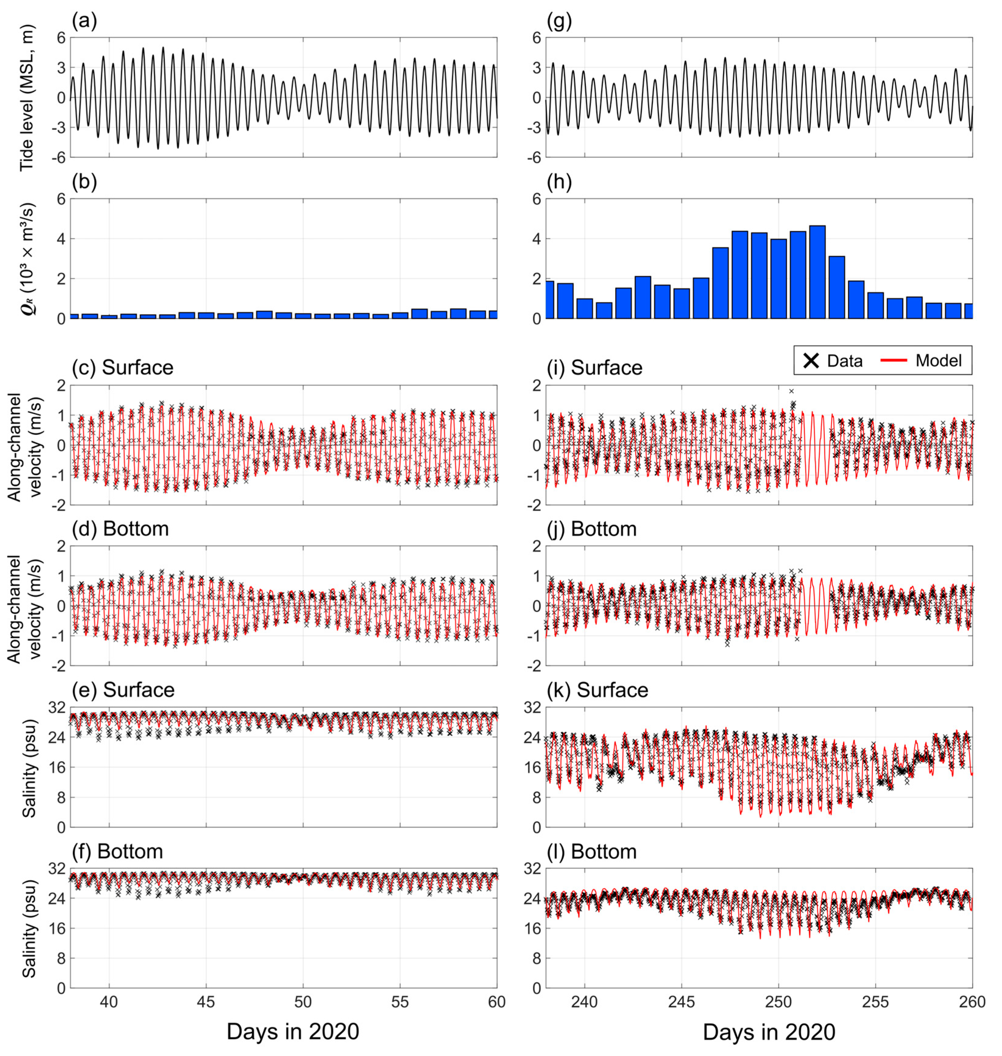
The along-channel velocity of the model reproduces the observed results well during both winter and summer with high predictive Skills of 0.95–0.99. ME and MAE represented the range from −25.77 to −2.33 cm/s and from 9.27 to 28.67 cm/s, respectively (Table 2). The tidal variation in current of about 0.5–1.2 m/s magnitude is almost similar to the observation results of Song et al. [38]. Although there is a distinct difference in river discharge between winter and summer (Figure 3b,h), the current patterns at M1 in both surface and bottom layers are not significantly affected by the variation in river discharge. It suggests that the current patterns in YC are considerably controlled by tidal variations.
Figure 3.
Model-data comparison for time series of current velocity and salinity during days 38–60 and days 238–260 in 2020. (a,g) Time series of tide level at T2, (b,h) daily river discharge from Han River, (c,d,i,j) time series of along-channel velocity at the near-surface and near-bottom layer at M1, and (e,f,k,l) time series of salinity at the near-surface and near-bottom layer at M1.
4.3. Salinity
The salinity data, collected through CTD at M1 (Figure 1), were compared with the model results during winter (Figure 3e,f) and summer (Figure 3k,l). ME and MAE represented the range from 0.01 to 1.39 psu and from 0.69 to 1.47 psu, respectively (Table 2). The model reproduces the tidal variations of observed salinity well with predictive Skills of 0.87–0.98, except that the model overestimates the salinity on days 40–47 in winter (Figure 3e,f). The overestimation of the model can be attributable to the tributaries near the YC not being applied to the model. Freshwater discharged from local tributaries has the potential to reduce salinity in the YC during ebb tide. Applying local tributaries to the model is limited because of the problem related to the grid resolution and the lack of data. Nevertheless, the model gives excellent reproducibility for seasonal variation in observed salinity. The model reproduces the significant decrease in salinity and strong stratification by high river discharge (>2000 m3/s) well in summer (Figure 3h,k,l).
The spatial salinity data for the six salinity stations (S1–S6 in Figure 1) during 2011–2020 was collected from the Korea Marine Environment Management Corporation (KOEM). The KOEM provides four snapshot salinity data for the surface and bottom layers in February, May, August, and November. Figure 4 shows the maximum–minimum ranges for salinity data of the surface and bottom layer at stations S1–S6 in February, May, and August during 2011–2020. The maximum–minimum range of salinity decreases from upstream (S1) to downstream (S6) of the YC. The low salinity in August is attributed to the high river discharge. The monthly averaged modeled salinity for each station in February, May, and August was calculated to compare with the observed data (red dotted lines in Figure 4). The model reproduced the spatial salinity distribution in the YC well within the maximum–minimum range of the observed data.
5. Mechanisms of Salt Transport
We analyzed the characteristics of salt transport through three cross sections (L1, L2, and L3 in Figure 1) in the YC using the results of FVCOM. The subtidal volume transport (Qf) and salt transport (FS) through cross section A are calculated for L1, L2, and L3 using:
where u is the normal velocity for the cross section, and S is salinity. The positive and negative values of u represent landward and seaward directions, respectively. < > indicates the 48 h low-pass filter. Both u and S are decomposed into three components, following Lerczak et al. [8]:
where ϕ refers to either u or S. A0 is the 48-h low-passed cross-sectional area. h is the mean depth for a particular cell of a cross section, and η is sea-level variation. ϕ is decomposed into tidally and cross-sectionally averaged component (ϕ0), tidally averaged and cross-sectionally varying component (ϕE), and tidally and cross-sectionally varying component (ϕT). The ϕ0 and ϕE are the subtidal components, and the ϕT is the tidal component. With this decomposition, the subtidal salt transport FS is given by:
where QfS0 is the advective salt transport due to subtidal volume transport. The subtidal volume transport (Qf) is decomposed into the Eulerian residual volume transport (QE) and Stokes drift volume transport (QS) [39]. The interaction between QE and QS controls the transport direction of QfS0. In general, QfS0 is regarded as the seaward salt transport due to QE by river discharge [5,7,8]. The QS, however, can be strengthened by tidal nonlinearity in the tide-dominated estuary with little river discharge, causing the landward QfS0 [23].
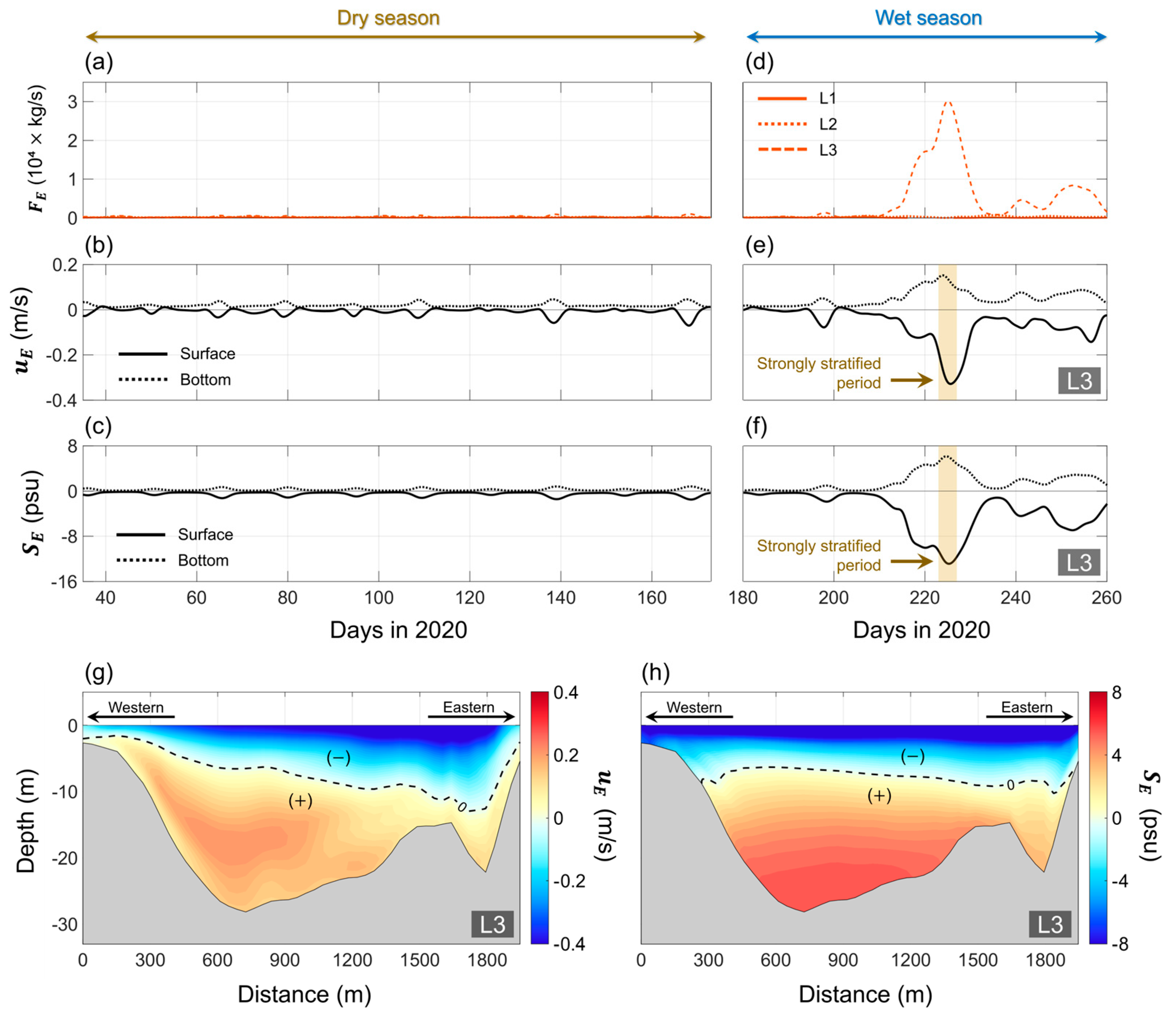
FE is the shear dispersive salt transport due to vertical current shear and vertical salinity gradient. FE is generally interpreted in terms of stratification and two-layer flow structure. In estuaries with strongly stratified conditions, the vertical gradient of estuarine exchange flow (uE) and salinity (SE) derive landward FE [5]. Therefore, FE provides the approximate information for estuarine type according to stratification intensity.
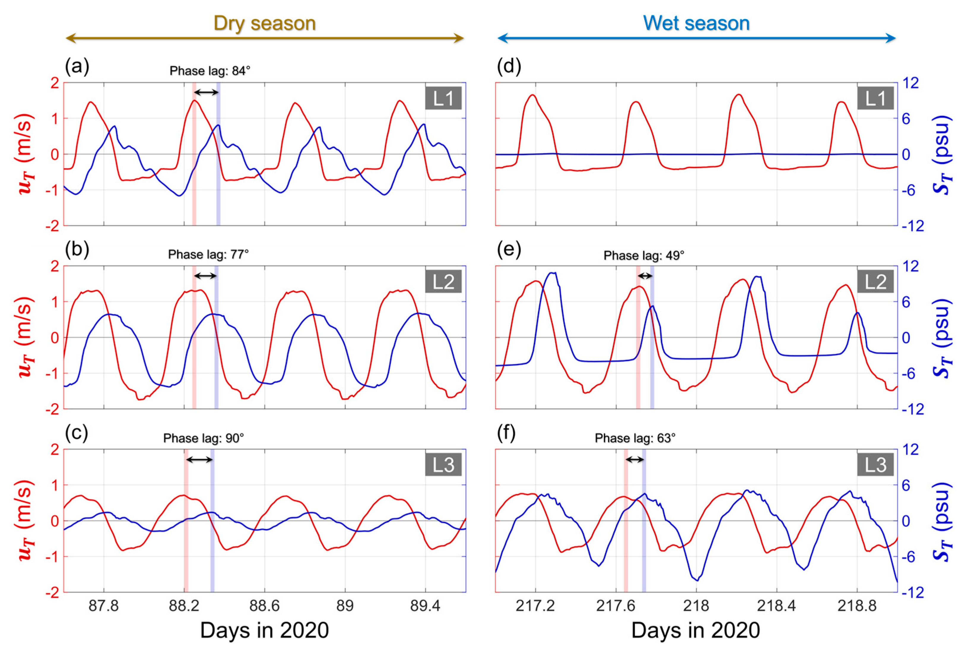
FT is the tidal oscillatory salt transport due to temporal correlations between tidal current (uT) and salinity (ST). uT and ST are the tidal components, so and are theoretically zero. However, various dispersive mechanisms such as tidal shear dispersion, tidal trapping, and tidal pumping induce not to be zero [12]. For example, the phase difference between uT and ST derived from the nonlinear effect of the tide can generate FT. The phase difference of less than 90° causes the landward FT, referred to as tidal trapping, whereas that of more than 90° causes the seaward FT [10,40]. In addition, each amplitude of uT and ST also significantly influences the strength of FT [9].
5.1. Variation in FS
We calculated FS and its three decomposed components QfS0, FE, and FT for L1, L2, and L3 cross sections to analyze the mechanism of salt transport by the interaction between tide and freshwater runoff in YC (Figure 5). There are 15 spring tides and 16 neap tides during the total analysis period of 225 days (Figure 5a). Days 35–172 are the dry season with river discharge of less than 500 m3/s, and days 180–260 are the wet season with river discharge of a maximum of 20,000 m3/s (Figure 5b). During the wet season, there are two high-discharge events: R1 with river discharge of 5000–20,000 m3/s and R2 with river discharge of 4000–4900 m3/s.
The temporal variation in tide and river discharge strongly influences the transport process of FS in YC. The tide effect controls FS in the dry season, whereas the river discharge controls FS in the wet season. During the dry season, FS shows a regular pattern with a period of about 14.76 days in all cross sections (Figure 5c–e). This period coincides with the period of the spring–neap cycle caused by the interaction between M2 and S2 constituents. This pattern gives landward and seaward FS in the spring and neap tides, respectively. However, no spring–neap cycle of FS is shown in the wet season. The high river discharge during the wet season changes the regular pattern of FS, mainly causing seaward FS. The averaged FS at L1, L2, and L3 during the period R1 were calculated as −98.2, −607.2, and −4208.1 kg/s, respectively. These distinct difference in FS between the dry and wet seasons is driven by several mechanisms. Therefore, it is necessary to analyze the characteristics of QfS0, FE, and FT, which are decomposed components of FS, to understand these mechanisms.
5.1.1. Variation in Qf and S0
During the dry season, both Qf and S0 show distinct spring–neap cycles in all cross sections (Figure 6b,c); S0 at the L3 closed to the open sea is an exception due to its constant salinity of about 31 psu. The pattern of QfS0 follows the pattern of Qf (Figure 6a). The fast Fourier transformation (FFT) of Qf during the dry season shows that the variation in Qf is controlled by the long-term tidal constituents MSf and Mm (Figure 6g–i). The fortnightly tide MSf with a period of 14.76 days is a compound tide produced by the interaction of M2 and S2. The Mm with a period of 27.55 days is a lunar monthly tide formed by the effect of irregularities in the orbital speed and orbit of the moon. Although the influence of these long-term tidal constituents in many estuaries is negligible, long-term tidal constituents in the tide-dominated estuary can play a significant role in the estuarine circulation system [13]. The weak river discharge during the dry season is the main factor that makes YC a tide-dominated estuary, strengthening the effect of long-term tidal constituents. As a result, QfS0 fluctuates by MSf and Mm (Figure 6a), causing the landward and seaward FS patterns in the dry season, respectively (Figure 5c–e).
During the wet season, the high river discharge in R1 and R2 increased the seaward Qf more than 20 times compared to the dry season, deforming its spring–neap cycle (Figure 6e). The salinity (S0) is decreased significantly in all cross sections due to the influence of freshwater (Figure 6f). The QfS0, influenced by seaward Qf, reaches −1.0 × 10⁴ and −4.5 × 10⁴ kg/s at the L2 and L3, respectively, during the R1 period (Figure 6d). In the case of L1, the QfS0 converges close to zero with S0 (Figure 6d,f), resulting in no salt transport FS (Figure 5f); FE and FT described later are also the same. It is due to the close distance between L1 and the freshwater source. Therefore, the pattern of QfS0 during the wet season, except for L1, shows long-term seaward transport due to the strong barotropic flow caused by the freshwater discharge (Figure 6d), resulting in the long-term seaward FS pattern (Figure 5g,h).
5.1.2. Variation in uE and SE
The FE in L1 and L2 has no significant effect on net salt transport FS. During the model simulation period, there are little variations of both uE and SE in L1 and L2 (not shown). The FE in L1 and L2 is less than 120 kg/s (Figure 7a,d). These results mean no two-layer flow structure and no stratification in L1 and L2, so the channel around L1 and L2 has characteristics of a well-mixed estuary regardless of river discharge.
The L3, however, is the region where FE is the most prominent on days 215–260 due to the high river discharge during R1 and R2 (Figure 7d). The peak of landward FE is related to the salinity stratification and the vertical current shear. The strong vertical gradient of uE and SE give the salinity stratification and two-layer flow structure [5,41]. The peak of FE can be more pronounced in the strongly stratified estuary, where freshwater discharge is stronger than the tidal forces. The high river discharge during R1 forms the strongly stratified period at the L3 on days 223–226 (yellow area in Figure 7e,f) with ∆uE of about 0.4 m/s and ∆SE of about 16 psu. Figure 7g,h shows the highly sheared two-layer flow structure and strongly stratified salinity distribution during the strongly stratified period. These results suggest that the high river discharge in YC can transform the feature of the estuary into a strongly stratified estuary at the L3. As a result, the strong ∆uE and ∆SE at the L3 during R1 increase the landward FE, peaking at 3.0 × 10⁴ kg/s (Figure 7d).
The variation in ∆uE and ∆SE due to the interaction between the tidal forces and freshwater discharge are also partially visible in the dry season. During neap tide, the magnitude of ∆uE and ∆SE is higher than spring tide due to its relatively weak tidal forces (Figure 7b,c). However, its magnitude can be relatively neglected because it is not large enough to influence the variation in FE.
5.1.3. Variation in uT and ST
The FT could be one of the factors causing the landward salt transport in YC. During the dry season, distinct variations in landward FT are seen at the L1 and L2 (Figure 5c,d). The landward FT at the L1 and L2 is caused by the phase difference between uT and ST being smaller than 90° (Figure 8a,b). These effects between the uT and ST are known as tidal trapping [10,12,40]. The landward FT derived from tidal trapping has a period of 14.76 days due to the spring–neap cycle of the uT and ranges from 200 to 2600 kg/s. The tidal trapping effect at the L3 during the dry season is relatively weaker than the L1 and L2 (Figure 8c), so the FT could be negligible at the L3 (Figure 5e). As a result, the variation in FS at the L1 and L2 fluctuates by the interaction between QfS0 and FT (Figure 5c,d), but the FS at the L3 is almost entirely determined by the QfS0 (Figure 5e).
The high freshwater discharge during the wet season enhances the tidal trapping effect and the amplitude of ST at the L2 and L3 (Figure 8e,f). Phase difference between uT and ST at the L2 and L3 during the wet season reduced to 49° and 63°, respectively. Moreover, the high river discharge enhances the horizontal gradient of the salinity, increasing the amplitude of ST. The high amplitude of ST combines with tidal trapping effects, resulting in stronger landward FT. These nonlinear effects of the tide at the L2 and L3 increase the FT, peaking at 0.7 × 10⁴ and 1.9 × 10⁴ kg/s, respectively (Figure 5g,h). The ST at the L1 has no variation during the wet season as the mean salinity is reduced to zero by high freshwater discharge (Figure 8d; see Section 5.1.1), resulting in no variation in FT.
Figure 8.
Tidal variation in uT and ST at L1, L2 and L3 during the dry season (a–c) and wet season (d–f). Positive and negative values in all figures indicate the landward and seaward direction, respectively.
Figure 8.
Tidal variation in uT and ST at L1, L2 and L3 during the dry season (a–c) and wet season (d–f). Positive and negative values in all figures indicate the landward and seaward direction, respectively.
5.2. Seasonal Variation in Salt Transport
We confirmed that the patterns of salt transport in YC are differentiated based on the dry and wet seasons. During the dry season, the patterns of salt transport fluctuated by the spring–neap cycle. However, the freshwater discharge during the wet season modified the salt transport patterns. Analysis of salt transport decomposition gave detailed mechanisms of these patterns.
The main mechanisms controlling FS during the dry season were the long-term tidal constituents (MSf and Mm) and the nonlinear effect of the tide by tidal trapping. The long-term tidal constituents caused the landward and seaward QfS0 during the spring and neap tides, respectively (Figure 6a). The tidal trapping effect continuously produced the landward FT (Figure 8a,b). Although FS was determined by the interaction between QfS0 and FT, its patterns almost followed the variation in QfS0 since the fluctuation range of QfS0 was stronger than FT. Therefore, the FS during the dry season repeated the landward and seaward transport patterns by the spring–neap cycle of the QfS0 varying by the long-term tidal constituents (Figure 5c–e).
The FS during the wet season had a distinct balance of the landward and seaward transport mechanisms. The strong barotropic flow by the freshwater discharge produced strong seaward QfS0 (Figure 6d). The stratification and two-layer flow structure caused the landward FE (Figure 7d). The tidal trapping effect enhanced by the freshwater discharge increased the landward FT (Figure 8e,f). These three components (QfS0, FE, and FT) interacted during the wet season and had higher values than during the dry season. However, the seaward QfS0 during the R1 and R2 exceeded the sum of landward FE and FT. Accordingly, the FS during the wet season was seaward due to the strong barotropic effect of QfS0 by the freshwater discharge (Figure 5g,h).
5.3. Unique Characteristics of Hypertidal Estuary
The main driving force of QfS0 in most estuaries is commonly known as freshwater runoff [5,7,8]. In addition, the effects of wind stress and sea level variation can affect the variation in QfS0 in some estuaries [5,42]. In the northern Gulf of Mexico estuary, for example, the onshore Ekman transport by the along-shelf wind events generates landward QfS0 [5]. And the changes in sea surface height caused by tropical storms in Delaware Bay on the east coast of the United States can also change the variation in QfS0 [42]. These studies suggested that QfS0 could be affected by other factors as well as freshwater runoff. Our research showed that the pattern of QfS0 was significantly influenced by the long-term tidal constituents MSf and Mm in the hypertidal estuary when freshwater runoff was sufficiently weak (Figure 6). It is known that the long-term tidal constituents have little influence compared to astronomical tides such as M2, S2, K1, O1, and N2, but it can be important in terms of the residual current of the tide-dominated estuary [13]. Accordingly, in the hypertidal estuary with low freshwater runoff conditions, the variation in QfS0 could be sufficiently strengthened by the long-term tidal constituents.
The high river discharge in many estuaries can increase landward FE as well as seaward QfS0 [5,11]. This characteristic was also found at the L3 cross section in YC during the wet season (Figure 5h). However, our research showed that the tidal trapping effect combined with high river discharge during the wet season increased landward FT (Figure 8). The high river discharge during the wet season significantly decreased the phase difference between tidal current and salinity. Moreover, the tidal variation in salinity (ST) was increased due to the freshwater discharge. These effects were combined with the strong tidal current (uT) in the YC and finally contributed to the increase in landward FT (Figure 5g,h). Therefore, the interaction between the nonlinear effect of the tide and high river discharge could be a factor that strengthens landward FT in the hypertidal estuary.
6. Conclusions
In this study, the salt transport mechanisms by the interaction between tide and river discharge in the YC were analyzed using the 3-D numerical model FVCOM. The salt transport was decomposed into three components through the Eulerian decomposition method. During the dry season, the salt transport patterns were mainly dominated by advective salt transport. During the wet season, the salt transport patterns were determined by the balance between advective salt transport, shear dispersion, and tidal oscillatory salt transport. Among these components, the mechanisms for advective and tidal oscillatory salt transport could be considered unique characteristics in a hypertidal estuary such as the YC.
The advective salt transport was characterized by the spring–neap variation during the dry season. The long-term tidal constituents MSf and Mm played a significant role in generating these variations. The variation in advective salt transport during the dry season caused the total salt transport in the YC to repeat the landward and seaward transport patterns. However, during the wet season, the effects on the long-term tidal constituents were not shown due to the strong barotropic flow by the high river discharge, resulting in continuous seaward advective salt transport. Nonetheless, since the dry season in GGB occupies most of the year, the variation in salt transport caused by the long-term tidal constituents could be the dominant process in the YC.
The tidal oscillatory salt transport was a factor that generates landward salt transport due to the tidal trapping effect by the phase difference of less than 90° in tidal current and salinity. This mechanism existed during both dry and wet seasons due to the nonlinear effect of the tide of the YC, although that was relatively weak during the dry season. The high river discharge during the wet season decreased the phase difference between tidal current and salinity to less than 70°, resulting in a much stronger landward tidal oscillatory salt transport. Thus, the nonlinear effect of the tide in the YC could be coupled with the freshwater runoff process, leading to significantly strong landward tidal oscillatory salt transport.
These unique characteristics in the YC could significantly contribute to research on material circulation in the tide-dominated estuary or the hypertidal estuary. In addition, FVCOM results for the YC showed that salt transport patterns were distinctly changed depending on the magnitude and variation in freshwater discharge from the land. Therefore, to accurately predict material transport mechanisms, it is necessary to conduct modeling of various scenarios of salt transport characteristics that change according to wide freshwater discharge ranges.
Author Contributions
Conceptualization, H.M.L., J.W.K. and S.-B.W.; methodology, H.M.L. and J.W.K.; software, visualization, and validation, H.M.L.; formal analysis, H.M.L. and J.W.K.; investigation, H.M.L., J.W.K. and S.-B.W.; resources, H.M.L. and S.-B.W.; data curation, H.M.L. and S.-B.W.; writing—original draft preparation, H.M.L., J.W.K. and S.-B.W.; writing—review and editing, H.M.L., J.W.K. and S.-B.W.; supervision, S.-B.W.; project administration, S.-B.W.; funding acquisition, S.-B.W. All authors have read and agreed to the published version of the manuscript.
Funding
This work was supported by Institute of Information & communications Technology Planning & Evaluation (IITP) grant funded by the Korea government (MSIT) (RS-2022-00155915, Artificial Intelligence Convergence Innovation Human Resources Development (Inha University)). This research was supported by a National Research Foundation of Korea Grant from the Korean Government (MSIT; the Ministry of Science and ICT) NRF-2021M1A5A1075516) (KOPRI-PN22013).
Institutional Review Board Statement
Not applicable.
Informed Consent Statement
Not applicable.
Data Availability Statement
Model results can be requested by contacting the corresponding author.
Conflicts of Interest
The authors declare no conflict of interest.
References
- Neilson, B.J.; Cronin, L.E. Estuaries and Nutrients; Humana Press: Clifton, NJ, USA, 1981. [Google Scholar]
- John, S.; Muraleedharan, K.R.; Revichandran, C.; Azeez, S.A.; Seena, G.; Cazenave, P.W. What controls the flushing efficiency and particle transport pathways in a tropical estuary? Cochin estuary, southwest coast of India. Water 2020, 12, 908. [Google Scholar] [CrossRef] [Green Version]
- Narayanan, N.C.; Venot, J.P. Drivers of Change in Fragile Environments: Challenges to Governance in Indian Wetlands. Nat. Resour. Forum 2009, 33, 320–333. [Google Scholar] [CrossRef]
- Jeong, H.; Kang, S.; Jung, H.; Jeong, D.; Oh, J.; Choi, S.; An, Y.; Choo, H.; Choi, S.; Kim, S.; et al. The Current Status of Eutrophication and Suggestions of the Purification & Restoration on Surface Sediment in the Northwestern Gamak Bay, Korea, 2017. J. Korean Soc. Mar. Environ. Energy 2019, 22, 105–113. [Google Scholar] [CrossRef]
- Kim, C.K.; Park, K. A Modeling Study of Water and Salt Exchange for a Micro-Tidal, Stratified Northern Gulf of Mexico Estuary. J. Mar. Syst. 2012, 96–97, 103–115. [Google Scholar] [CrossRef]
- Devkota, J.; Fang, X. Quantification of Water and Salt Exchanges in a Tidal Estuary. Water 2015, 7, 1769–1791. [Google Scholar] [CrossRef] [Green Version]
- Gong, W.; Shen, J. The Response of Salt Intrusion to Changes in River Discharge and Tidal Mixing during the Dry Season in the Modaomen Estuary, China. Cont. Shelf Res. 2011, 31, 769–788. [Google Scholar] [CrossRef]
- Lerczak, J.A.; Geyer, W.R.; Chant, R.J. Mechanisms Driving the Time-Dependent Salt Flux in a Partially Stratified Estuary. J. Phys. Oceanogr. 2006, 36, 2296–2311. [Google Scholar] [CrossRef] [Green Version]
- Li, R.; Gao, L.; Pan, C.; Pang, Y. Detecting the Mechanisms of Longitudinal Salt Transport during Spring Tides in Qiantang Estuary. J. Integr. Environ. Sci. 2019, 16, 123–140. [Google Scholar] [CrossRef] [Green Version]
- Wang, T.; Geyer, W.R.; Engel, P.; Jiang, W.; Feng, S. Mechanisms of Tidal Oscillatory Salt Transport in a Partially Stratified Estuary. J. Phys. Oceanogr. 2015, 45, 2773–2789. [Google Scholar] [CrossRef] [Green Version]
- Monismith, S.G.; Kimmerer, W.; Burau, J.R.; Stacey, M.T. Structure and flow-induced variability of the subtidal salinity field in northern San Francisco Bay. J. Phys. Oceanogr. 2002, 32, 3003–3019. [Google Scholar] [CrossRef]
- Fischer, H.B.; List, J.E.; Koh, C.R.; Imberger, J.; Brooks, N.H. Mixing in Inland and Coastal Waters; Academic Press: San Diego, CA, USA, 1979. [Google Scholar]
- Garel, E.; Zhang, P.; Cai, H. Dynamics of Fortnightly Water Level Variations along a Tide-Dominated Estuary with Negligible River Discharge. Ocean Sci. 2021, 17, 1605–1621. [Google Scholar] [CrossRef]
- Suh, S.W.; Lee, H.Y.; Kim, H.J. Spatio-Temporal Variability of Tidal Asymmetry Due to Multiple Coastal Constructions along the West Coast of Korea. Estuar. Coast. Shelf Sci. 2014, 151, 336–346. [Google Scholar] [CrossRef]
- Woo, S.B.; Il Yoon, B. Numerical Simulation of Fortnightly Modulations of the Convergence Zone by Residual Volume Transport in a Macrotidal Estuary. J. Coast. Res. 2018, 85, 606–610. [Google Scholar] [CrossRef]
- Yoon, B.; Woo, S.-B. Tidal Asymmetry and Flood/Ebb Dominance around the Yeomha Channel in the Han River Estuary, South Korea. J. Coast. Res. 2013, 165, 1242–1246. [Google Scholar] [CrossRef]
- Yoon, B.I.; Woo, S.-B.; Kim, J.W.; Song, J. Il. The Regional Classification of Tidal Regime Using Characteristics of Astronomical Tides, Overtides and Compound Tides in the Han River Estuary, Gyeonggi Bay. J. Korean Soc. Coast. Ocean Eng. 2015, 27, 149–158. [Google Scholar] [CrossRef]
- Kang, C.H.; Oh, S.J.; Shin, Y.J.; Kim, Y.G.; Oh, E.G.; So, J.S. Impact of Inland Pollution Sources on the Bacteriological Water Quality of the Southern Ganghwado Bay Area, South Korea. Urban Water J. 2017, 14, 69–73. [Google Scholar] [CrossRef]
- Kim, D.Y.; Yoon, C.G.; Rhee, H.P.; Choi, J.H.; Hwang, H.S. Estimation of Pollution Contribution TMDL Unit Watershed in Han-River according to Hydrological Characteristic using Flow Duration Curve. J. Korean Soc. Water Environ. 2019, 35, 497–509. [Google Scholar] [CrossRef]
- Lim, D.I.; Rho, K.C.; Jang, P.G.; Kang, S.M.; Jung, H.S.; Jung, R.H.; Lee, W.C. Temporal-Spatial Variations of Water Quality in Gyeonggi Bay, West Coast of Korea, and Their Controlling Factor. Ocean Polar Res. 2007, 29, 135–153. [Google Scholar] [CrossRef] [Green Version]
- Lee, D.-H.; Yoon, B.-I.; Kim, J.-W.; Gu, B.-H.; Woo, S.-B. The Cross-Sectional Mass Flux Observation at Yeomha Channel, Gyeonggi Bay at Spring Tide During Dry and Flood Season. J. Korean Soc. Coast. Ocean Eng. 2012, 24, 16–25. [Google Scholar] [CrossRef]
- Lee, D.H.; Yoon, B.I.; Woo, S.-B. The Cross-Sectional Characteristic and Spring-Neap Variation of Residual Current and Net Volume Transport at the Yeomha Channel. J. Korean Soc. Coast. Ocean Eng. 2017, 29, 217–227. [Google Scholar] [CrossRef] [Green Version]
- Park, K.; Oh, J.H.; Kim, H.S.; Im, H.H. Case study: Mass Transport Mechanism in Kyunggi Bay around Han River Mouth, Korea. J. Hydraul. Eng. 2002, 128, 257–267. [Google Scholar] [CrossRef]
- Yoon, B.-I.; Woo, S.-B. Relation of Freshwater Discharge and Salinity Distribution on Tidal Variation around the Yeomha Channel, Han River Estuary. J. Korean Soc. Coast. Ocean Eng. 2012, 24, 269–276. [Google Scholar] [CrossRef] [Green Version]
- Lee, H.M.; Kim, J.W.; Choi, J.Y.; Yoon, B.I.; Woo, S.-B. Mechanisms of Salt Transport in the Han River Estuary, Gyeonggi Bay. J. Korean Soc. Coast. Ocean Eng. 2021, 33, 13–29. [Google Scholar] [CrossRef]
- Yang, E.J.; Choi, J.K.; Hyun, J.H. Seasonal Variation in the Community and Size Structure of Nano- and Microzooplankton in Gyeonggi Bay, Yellow Sea. Estuar. Coast. Shelf Sci. 2008, 77, 320–330. [Google Scholar] [CrossRef]
- Chen, C.; Liu, H.; Beardsley, R.C. An Unstructured Grid, Finite-Volume, Three-Dimensional, Primitive Equations Ocean Model: Application to Coastal Ocean and Estuaries. J. Atmos. Ocean. Technol. 2003, 20, 159–186. [Google Scholar] [CrossRef]
- Chen, C.; Qi, J.; Li, C.; Beardsley, R.C.; Lin, H.; Walker, R.; Gates, K. Complexity of the Flooding/Drying Process in an Estuarine Tidal-Creek Salt-Marsh System: An Application of FVCOM. J. Geophys. Res. Oceans 2008, 113, C07052. [Google Scholar] [CrossRef] [Green Version]
- Mellor, G.L.; Yamada, T. Development of a Turbulence Closure Model for Geophysical Fluid Problems. Rev. Geophys. 1982, 20, 851–875. [Google Scholar] [CrossRef] [Green Version]
- Smagorinsky, J. General Circulation Experiments with the Primitive Equations: I. The Basic Experiment. Mon. Weather Rev. 1963, 91, 99–164. [Google Scholar] [CrossRef]
- Chen, C.; Zhu, J.; Zheng, L.; Ralph, E.; Budd, J.W. A Non-Orthogonal Primitive Equation Coastal Ocean Circulation Model: Application to Lake Superior. J. Great Lakes Res. 2004, 30, 41–54. [Google Scholar] [CrossRef]
- Chen, C.; Beardsley, R.C.; Cowles, G. An Unstructured-Grid, Finite-Volume Coastal Ocean Model (FVCOM) System. Oceanography 2006, 19, 78–89. [Google Scholar] [CrossRef] [Green Version]
- Chen, C.; Huang, H.; Beardsley, R.C.; Liu, H.; Xu, Q.; Cowles, G. A Finite Volume Numerical Approach for Coastal Ocean Circulation Studies: Comparisons with Finite Difference Models. J. Geophys. Res. Oceans 2007, 112, C03018. [Google Scholar] [CrossRef]
- Cowles, G.W.; Lentz, S.J.; Chen, C.; Xu, Q.; Beardsley, R.C. Comparison of Observed and Model-Computed Low Frequency Circulation and Hydrography on the New England Shelf. J. Geophys. Res. Oceans 2008, 113, C09015. [Google Scholar] [CrossRef] [Green Version]
- Chen, C.; Beardsley, R.C.; Cowles, G.; Qi, J.; Lai, Z.; Gao, G.; Stuebe, D.; Liu, H.; Xue, P.; Ge, J.; et al. An Unstructured Grid, Finite-Volume Community Ocean Model FVCOM User Manual; SMAST/UMASSD Technical Report-13-0701; Massachusetts Institute of Technology: Cambridge, MA, USA, 2011. [Google Scholar]
- Egbert, G.D.; Erofeeva, S.Y. Efficient Inverse Modeling of Barotropic Ocean Tides. J. Atmos. Ocean. Technol. 2002, 19, 183–204. [Google Scholar] [CrossRef]
- Willmott, C.J. Some Comments on the Evaluation of Model Performance. Bull. Am. Meteorol. Soc. 1982, 63, 1309–1313. [Google Scholar] [CrossRef]
- Song, Y.-S.; Woo, S.-B. Periodic Characteristics of Long Period Tidal Current by Variation of the Tide Deformation around the Yeomha Waterway. J. Korean Soc. Coast. Ocean Eng. 2011, 23, 393–400. [Google Scholar] [CrossRef]
- Sylaios, G.; Boxall, S.R. Residual Currents and Flux Estimates in a Partially-Mixed Estuary. Estuar. Coast. Shelf Sci. 1998, 46, 671–682. [Google Scholar] [CrossRef] [Green Version]
- MacVean, L.J.; Stacey, M.T. Estuarine Dispersion from Tidal Trapping: A New Analytical Framework. Estuaries Coasts 2011, 34, 45–59. [Google Scholar] [CrossRef] [Green Version]
- Choi, N.-Y.; Yoon, B.-I.; Kim, J.-W.; Song, J.-I.; Lim, E.-P.; Woo, S.-B. The Relation of Cross-Sectional Residual Current and Stratification during Spring and Neap Tidal Cycle at Seokmo Channel, Han River Estuary Located at South Korea. J. Korean Soc. Coast. Ocean Eng. 2012, 24, 149–158. [Google Scholar] [CrossRef] [Green Version]
- Aristizábal, M.F.; Chant, R.J. An Observational Study of Salt Fluxes in Delaware Bay. J. Geophys. Res. Oceans 2015, 120, 2751–2768. [Google Scholar] [CrossRef]
Figure 1.
Computational grid and bathymetry of Gyeonggi Bay (a) and Yeomha Channel (b), and depth variation along the Y1–Y2 line (c), showing eight tide stations T1–T8 from KHOA (sky-blue squares), six salinity stations S1–S6 from KOEM (green triangles), and mooring station M1 (red ). The Y1–Y2 line contains three analysis cross sections (L1–L3).
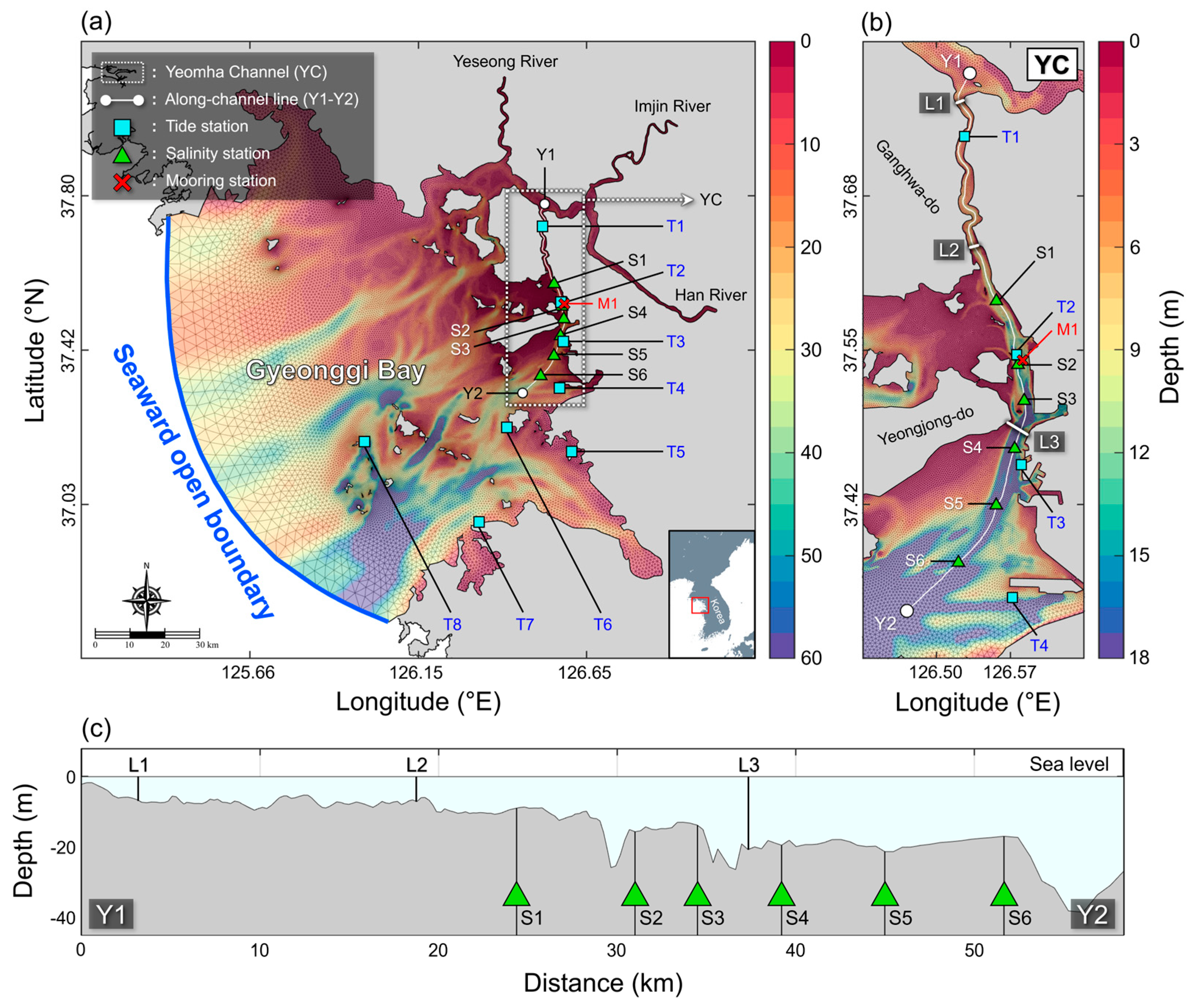
Figure 2.
Model-data comparison for tide level and harmonic constants during days 33–78 in 2020. (a–c) Time series of tide level at T1, T2 and T3, and (d–e) harmonic constants for five tidal constituents at T1–T8 [25].
Figure 2.
Model-data comparison for tide level and harmonic constants during days 33–78 in 2020. (a–c) Time series of tide level at T1, T2 and T3, and (d–e) harmonic constants for five tidal constituents at T1–T8 [25].

Figure 4.
Model-data comparison of spatial salinity distribution for the surface (a–c) and bottom layer (d–f) at S1–S6. The error bars show the maximum–minimum range of observed salinity data over 10 years for February, May, and August, respectively. The red dots indicate monthly averaged model data for salinity in February, May, and August, respectively.

Figure 5.
Variation in salt transport at L1, L2 and L3: (a) Time series of tide level at T2, (b) daily river discharge from Han River, (c–h) salt transport FS and its three decomposed components QfS0, FE and FT through L1, L2 and L3. Positive and negative values in (c–h) indicate the landward and seaward transport, respectively.

Figure 6.
Variation in (a,d) advective salt flux QfS0, (b,e) volume transport Qf and (c,f) cross-sectionally averaged salinity S0 at L1, L2 and L3. (g–i) FFT analysis of Qf during days 41–159 (green area in (b)), showing two major signals—MSf and Mm. Positive and negative values in (a,b,d,e) indicate the landward and seaward transport, respectively.
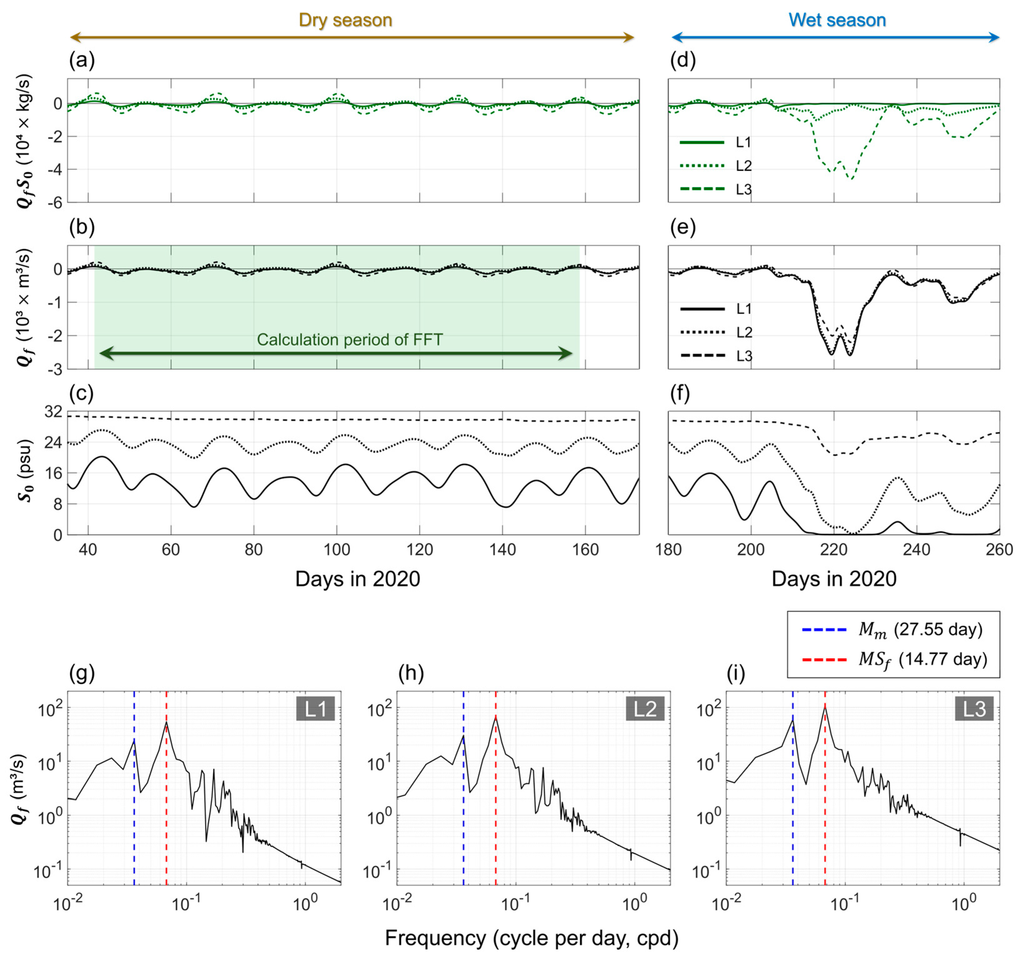
Figure 7.
Variation in (a,d) shear dispersion FE, (b,e) subtidal estuarine exchange flow uE and (c,f) salinity SE for the surface and bottom layers at L3. (g–h) The lateral and vertical distribution of uE and SE during strongly stratified period (yellow areas in (e–f)). Positive and negative values in (a–f) indicate the landward and seaward transport, respectively.

Table 1.
Setup details for ADCP and CTD instruments [25].
Table 1.
Setup details for ADCP and CTD instruments [25].
| Instruments | Setup Values | Winter | Summer | |
|---|---|---|---|---|
| ADCP | Bin size (m) | 0.50 | 0.50 | |
| Ping interval (sec) | 0.50 | 0.50 | ||
| Burst interval (min) | 10 | 10 | ||
| Blanking depth (m) | 0.20 | 0.20 | ||
| Deployment depth (m) | 0.47 | 0.47 | ||
| CTD | Surface | Sampling interval (min) | 10 | 10 |
| Depth below surface (m) | 4 | 3.5 | ||
| Bottom | Sampling interval (min) | 10 | 10 | |
| Deployment depth (m) | 0.27 | 0.27 | ||
Table 2.
Error estimates for model validation of tide level, current velocity, and salinity [25].
Table 2.
Error estimates for model validation of tide level, current velocity, and salinity [25].
| Seasons | Variables | Station | Location | Observation Periods | ME | MAE | Skill | ||
|---|---|---|---|---|---|---|---|---|---|
| Winter | Tide–level (cm) | T1 | 37°43′55″ N 126°31′20″ E | 1/20~3/20 in 2020 | 1.34 | 23.52 | 0.99 | ||
| T2 | 37°32′44″ N 126°35′3″ E | 1.47 | 21.10 | 0.99 | |||||
| T3 | 37°27′7″ N 126°35′32″ E | 1.41 | 20.14 | 0.99 | |||||
| T4 | 37°20′17″ N 126°35′10″ E | 1.46 | 19.67 | 0.99 | |||||
| T5 | 37°11′3″ N 126°37′41″ E | 1.52 | 18.69 | 0.99 | |||||
| T6 | 37°0′27″ N 126°21′10″ E | 1.71 | 17.95 | 0.99 | |||||
| T7 | 37°14′19″ N 126°25′43″ E | 1.65 | 18.41 | 0.99 | |||||
| T8 | 37°11′43″ N 125°59′47″ E | 1.76 | 18.89 | 0.99 | |||||
| Along–channel velocity (cm/s) | Surface | M1 | 37°32′28″ N 126°34′58″ E | 2/04~3/17 in 2020 | −2.33 | 10.62 | 0.99 | ||
| Bottom | −3.90 | 9.27 | 0.99 | ||||||
| Salinity (psu) | Surface | 0.94 | 0.94 | 0.87 | |||||
| Bottom | 0.67 | 0.69 | 0.88 | ||||||
| Summer | Along–channel velocity (cm/s) | Surface | 8/22~9/21 in 2020 | −25.77 | 28.67 | 0.95 | |||
| Bottom | −10.99 | 18.25 | 0.97 | ||||||
| Salinity (psu) | Surface | 0.01 | 0.98 | 0.98 | |||||
| Bottom | 1.39 | 1.47 | 0.90 | ||||||
Disclaimer/Publisher’s Note: The statements, opinions and data contained in all publications are solely those of the individual author(s) and contributor(s) and not of MDPI and/or the editor(s). MDPI and/or the editor(s) disclaim responsibility for any injury to people or property resulting from any ideas, methods, instructions or products referred to in the content. |
© 2023 by the authors. Licensee MDPI, Basel, Switzerland. This article is an open access article distributed under the terms and conditions of the Creative Commons Attribution (CC BY) license (https://creativecommons.org/licenses/by/4.0/).
Share and Cite
MDPI and ACS Style
Lee, H.M.; Kim, J.W.; Woo, S.-B. Mechanisms of Advective and Tidal Oscillatory Salt Transport in the Hypertidal Estuary: Yeomha Channel in Gyeonggi Bay. J. Mar. Sci. Eng. 2023, 11, 287. https://doi.org/10.3390/jmse11020287
AMA Style
Lee HM, Kim JW, Woo S-B. Mechanisms of Advective and Tidal Oscillatory Salt Transport in the Hypertidal Estuary: Yeomha Channel in Gyeonggi Bay. Journal of Marine Science and Engineering. 2023; 11(2):287. https://doi.org/10.3390/jmse11020287
Chicago/Turabian StyleLee, Hye Min, Jong Wook Kim, and Seung-Buhm Woo. 2023. "Mechanisms of Advective and Tidal Oscillatory Salt Transport in the Hypertidal Estuary: Yeomha Channel in Gyeonggi Bay" Journal of Marine Science and Engineering 11, no. 2: 287. https://doi.org/10.3390/jmse11020287
Note that from the first issue of 2016, this journal uses article numbers instead of page numbers. See further details here.