Article

RANS-Based Modelling of Turbulent Flow in Submarine Pipe Bends: Effect of Computational Mesh and Turbulence Modelling

1
State Key Laboratory of Hydroscience and Engineering, Tsinghua University, Beijing 100084, China
2
Department of Civil and Environmental Engineering, Politecnico di Milano, 20133 Milan, Italy
3
Key Laboratory of Geological Safety of Coastal Urban Underground Space, Ministry of Natural Resources, Qingdao 266100, China
4
Qingdao Geo-Engineering Surveying Institute, Qingdao Geological Exploration Development Bureau, Qingdao 266100, China
5
Qingdao Product Quality Testing Research Institute, Qingdao Product Quality Testing Technology Institute, Qingdao 266000, China
6
College of Environmental Science and Engineering, Ocean University of China, Qingdao 266100, China
*
Author to whom correspondence should be addressed.
J. Mar. Sci. Eng. 2023, 11(2), 336; https://doi.org/10.3390/jmse11020336
Submission received: 5 January 2023 / Revised: 17 January 2023 / Accepted: 20 January 2023 / Published: 3 February 2023
(This article belongs to the Special Issue Computational Fluid Mechanics II)

Abstract

:
Pipe bend is a critical integral component, widely used in slurry pipeline systems involving various engineering applications, including natural gas hydrate production. The aim of this study is to assess the capability of RANS-based CFD models to capture the main features of the turbulent single-phase flow in pipe bends, in view of the future investigation of the hydrate slurry flow in the same geometry. This is different from the available literature in which only a few accounted for the effects of a combination of computational mesh, turbulence model, and near-wall treatment approach. In this study, three types of mesh configuration were adopted to carry out the computations, namely unstructured mesh and two structured meshes with a uniform and nonuniform inflation layer, respectively. To explore the influence of the turbulence model, standard k-ε, low-Reynolds k-ε, and nonlinear eddy viscosity turbulence model were selected to close RANS equations. Pressure coefficient, mean axial velocity, turbulence intensity, secondary flow velocity, and magnitude of secondary flow were regarded as the critical variables to make a comprehensive sensitivity analysis. Predicted results suggest that turbulent kinetic energy is the most sensitive variable to the computational mesh while others tend to stabilize. The largest difference of turbulence kinetic energy was around 26% between unstructured mesh and structured mesh with a nonuniform inflation layer. Additionally, a fully resolved boundary layer can reduce the sensitivity of mesh on turbulent kinetic energy, especially for a nonlinear turbulence model. However, the large gradient and peak value of turbulence intensity near the inner wall of the bend was not captured by the case with a fully resolved boundary layer, compared with that of the wall function used. Furthermore, it has been confirmed that the same rule was detected also for different curvature ratios, Reynolds numbers, and dimensionless wall distance y+.

1. Introduction

A pipeline system is of paramount value for the transportation of natural gas hydrate slurry (NGHS). A pipe bend is one of the commonly used fitting components in slurry pipeline systems and hydrodynamic devices due to the flexibility of redirecting the flow. As known, even in the condition of dilute flow, excessive wear might happen at the outer wall due to the impingement of moving particles, which in turn results in a risk of leakage. Furthermore, pipe bends also induce excessive head loss related to the solid concentration. Disposing of tools for the prediction of the characteristics of the slurry flow inside the bend, as well as for the prediction of the induced loss of material, allows for the helping of the design and optimization of the slurry system. Computational fluid dynamics (CFD), an analysis of systems involving fluid flow, heat transfer, and associated phenomena such as chemical reactions by means of a computer-based simulation, provides a great opportunity in this sense, mostly since this approach has few limitations with respect to capital, scale, and measurement issues in laboratory tests. Simultaneously, numerical and modelling issues associated with CFD modelling have to be of concern.
To reduce the computational effort in most industrial applications, some averaging operator is usually applied to local instantaneous Navier-Stokes equations yielding the locally averaged quantities of the slurry flow, such as mean velocity and pressure fields, which raises nontrivial doubts regarding the proper type of averaging operator to apply and the modelling of the correlations arising from the averaging process. These aspects are still the subject of discussions among slurry flow modellers, however, no definite answer has been given even for the simplest case of single-phase incompressible flow. This is the consequence, on one hand, of the complexity of the turbulent flow inside a pipe bend and, on the other, of the strong assumptions underlying the Reynolds-Averaged Navier-Stokes (RANS) approach.
However, addressing the numerical simulation of the slurry flow in a certain geometry requires a clear understanding of how to model the same type of flow in the absence of particles. This is mainly due to two reasons. First of all, the single-phase flow can be interpreted as the limiting case of a slurry flow when the solid concentration tends to zero, and, therefore, slurry CFD models must be consistent with the single-phase ones. Second, the modelling of some of the correlations in slurry CFD models is usually performed via two-phase extensions of the commonly used turbulence models for single-phase flows. As a result, the goal of this study is to shed light on the capability of RANS-based CFD models to capture the physical processes of the turbulent single-phase flow in pipe bends, in light of the future investigation of the slurry flow in the same geometry. It should be mentioned that several studies adopted the large eddy simulation (LES) for simulating the turbulent flow in pipe bends with much more computational effort and more accurate results [1,2]. However, the LES approach is beyond the scope of this study since the goal is to provide the theoretical basis for the two-phase flow modeling where the RANS-based modelling is still applied.
Undoubtedly, more or less than half of the time spent on the CFD simulations is devoted to the preprocessing procedure, in particular, geometry building and mesh generation since the number and even shape of the grid can influence the convergence and stability of numerical simulation, finally resulting in an inaccurate solution. Generally, structured mesh composed of a quadrilateral in 2D and a hexahedron in 3D, respectively, is first used to discrete the numerical domain for the simple geometries. Gradually, the flow in complex geometry must be investigated and the unstructured mesh created, including a triangle in 2D, and a tetrahedron, prism, and pyramid in 3D. Despite the flexibility of unstructured mesh applied to a wide range of geometries, the structured mesh is still popular nowadays for the reason that a structured grid can be simply addressed by using the indices (i, j, and k) and the connectivity of a neighbour cell is very clear. Apart from this, governing equations can be solved by means of a straightforward solution algorithm without requiring the implementation of extra terms, provided that the grid is nearly orthogonal and without skewness. Conversely, once the grid is highly nonorthogonal, structured mesh might lead to an unphysical result, as the additional algorithms concerning the nonorthogonal issue have to be added which, in turn, results in numerical instability and divergence. In terms of an unstructured grid, a higher number of cells is needed to achieve the same accuracy, implying that a larger computational effort is required, compared with the structured mesh. In light of a case such as turbulent flow in a pipe bend, the boundary layer near the pipe wall might have a certain effect on the whole domain due to the large variety of variables here. For this reason, boundary layer resolution should also be considered with the application of a finer mesh near the wall to satisfy the log law of the wall or a fully resolved boundary layer up to the viscous sublayer.
In general, fluid particles pass through a curved surface, such as a bend, which is mainly characterized by secondary flow, axial flow separation, and unsteadiness. Here a secondary flow occurs in both the laminar and turbulence states resulting from the imbalance of pressure gradient at the radial direction of the bend cross-section and the centrifugal force produced by the curved geometry, referring to a pair of counter-rotating vortices determined by the Dean number, which is also called the Dean vortex [3]. With this type of pressure-driven secondary flow superimposing on the primary flow, the primary streamwise flow is distorted to a large extent. The faster fluid is transferred from the inner part of the bend through the centerline of the cross-section to the outer side of the bend while the fluid with a lower momentum to the inner section is along the top and bottom wall. In the case of a fully developed pipe bend flow, such as that occurring, for instance, in long coiled pipes, the velocity field will be the same for every cross-section. Conversely, when a bend of finite length is installed within two straight pipes, the characteristics of the primary and secondary flows will change along the pipe centerline. In order to describe such a system, similar to Sudo et al. [4], the most straightforward coordinate system seems to be a combined cylindrical-toroidal one, as demonstrated in Figure 1, in which the axial positions of the cross-sections of the upstream pipe, the bend, and the downstream pipe are identified, respectively, by the distance from the bend inlet section, z , the angle from the bend inlet section, φ , and the distance from the bend outlet section, z . Then, the points of each cross-section are identified by an azimuthal coordinate, θ , and a radial coordinate r. Therefore, based on the above considerations, the primary and secondary flow patterns are expected to vary with z , φ , and z . In some situations, the primary flow separates from the intrados of the pipe bend, giving rise to a streamwise vortex, provided that the curvature ratio defined as the proportion of curvature radius and pipe diameter Rc/d is less than 1.5 [5,6]. Clearly, the complex fluid dynamic behavior of pipe bend flows, especially in the turbulent regime, makes obtaining accurate, whole-field experimental data a very challenging task, especially in terms of velocity measurements.
To date, the turbulent flow through a pipe with a 90° or 180° bend has been widely explored by experimental and numerical approaches since it is of paramount importance to industrial practice. A comprehensive literature review on the studies of a curved pipe or channel from a historical point of view can be found in reference [7]. To the authors’ knowledge, the first research on the curved pipe can be dated back to 1855. Weisbach [8] carried out the experiment to measure the pressure loss in a sharp pipe bend. Followed by Weisbach, Thomson [9,10] pointed out that the difference between the flow in a curved pipe and wingding of the river and the secondary flow is induced by the imbalance of the pressure gradient and the centrifugal force. Williams et al. [11] first illustrated that the maximum mean velocity at the bend exit is displaced to the outer part of the pipe. Eustice [12,13] demonstrated that the pressure drop in a pipe bend is larger than that of a straight pipe. It is accepted that in one of the most notable works made by Dean [3,14], one pair of counter-rotating vortices were analytically calculated for laminar flow in a long pipe bend, which is determined by a parameter, namely the Dean number. Due to the limitation of the apparatus, the above-mentioned investigations are almost carried out in the laminar condition. With the development of measurement instruments, laser doppler velocimetry (LDV) and hot-wire anemometry have been applied to measure the mean quantities and turbulence statistics for three-dimensional components. Adler [15] first showed the mean velocity profiles and contours at a range of Reynolds numbers from 2000 to 12,000. Weske [5] conducted a series of experiments, aimed at exploring the velocity distribution along pipe bends for different types of cross-sections, such as circular, elliptical, square, and rectangular shapes. It was suggested that the shape and aspect ratio of the cross-section of the pipe have little effect on the mean velocity compared with the influence of the curvature ratio. Rowe [16] used a Pitot tube and yawmeter to measure the total pressure and yaw for a flow in the U bend and S bend. It was found that the secondary flow in a U bend started from 30° and decreased gradually until 90°. Then it became steady until the bend exit. In comparison to the U bend, the fully developed flow recovered faster downstream of the S bend. In order to further fully understand the profile of the flow, the longitudinal, circumferential, and radial components of mean and fluctuating velocities, and the Reynolds stresses in the pipe cross-section at several longitudinal stations were measured by using the technique of hot wire [4,17], extending the works of Enayet et al. [18] and Azzola et al. [19], who limited their investigations to measuring only the longitudinal and circumferential velocity components.
At the same time, the turbulent flow in pipe bends has been the subject of several numerical investigations, helped by the growing capabilities of computers and multipurpose CFD codes. However, a distinction shall be made according to the turbulence modelling approach and the purpose of the study. In the initial stage, based on the finite difference method, Patankar et al. [20] solved RANS equations with the closure of the standard k-ε turbulence model to predict the turbulent flow in a U bend, referring to the measurements made by Rowe [21]. They claimed that the calculations were not in good agreement with experimental data due to the isotropic property of the eddy viscosity model. Al-Rafai [22] investigated the effect of the curvature ratio on the streamwise velocity and RSM velocity via experimental and numerical techniques. In their simulation, the polar mesh was utilized to discretize the domain based on the body-fitted coordinates employed onto PHOENICS. The numerical results qualitatively agree with the measured data while having a significant quantitative deviation when it comes to the mean axial velocity. Both methods proved that the secondary flow in a sharper bend is more intense. Lai et al. [23] took into account the influence of boundary layer resolution for the Reynolds stress model (RSM) on a simulation of turbulent flow in a U bend. Two high-Reynolds RSM turbulence models, different from the pressure-strain model, with the application of wall function, have worse performance in predicting the third cell, normal stress, and downstream recovery than is the case with the low-Reynolds RSM turbulence model, which indicates that a fully resolved viscous sublayer results in a more accurate solution. Note that the grid-independent analysis for two polar meshes was also performed in their study, however, only the mean velocities profile and the in-plane velocity of 67.5° were considered. Also, Wang and Shirazi [24] utilized polar mesh to predict the characteristics of flow in a 90° bend with high and low-Reynolds k-ε turbulence models. In contrast to Lai et al. [23], the low-Reynolds k-ε model with a fully resolved boundary has a slight improvement in predicting the axial velocity at the outer wall of the bend. In terms of grid influence, the mean axial velocity at 30° for two polar meshes was compared. Note that they only doubled the cell number of the radial direction and claimed the difference between the results from refined mesh and experimental data was less than 1~2%, which does not seem reliable to make grid independence. Pruvost et al. [25] further carried out various simulations to investigate the influence of boundary resolution and turbulence models on the flow profile in a 90° and a 180° bend, respectively, using a structured hexahedron grid in circumferential, and an unstructured hexahedron grid in the core region. The grid convergence was achieved by solely comparing the mean axial velocity and turbulence kinetic energy at the bend exit with different mesh sizes. Similar to Wang and Shirazi [24], it was concluded that there was little improvement for the 90° bend after the fully resolved boundary layer (dimensionless wall distance was around one), regarding the mean axial velocity and static wall pressure. However, the performance of the model with a fully resolved boundary layer has obvious improvement for 180° bend, compared with those cases where the wall function was applied. A structured hexahedron mesh with four corners having bad orthogonality has been used to simulate double bend flow, incorporating standard k-ε and renormalization group (RNG) turbulence models [26]. Both models gave satisfactory results for mean axial velocity and the existence of a vortex, whereas the RNG model performed rather better in predicting tangential velocity than the standard k-ε model. Nevertheless, the case with the RNG model occupied four times the computer resources than that of the standard k-ε model. Kim et al. [27] selected an automatically generated unstructured hexahedron grid to computationally reproduce the experiments of Sudo et al. [4] in order to find an optimum turbulence model and further verify their data. Wang et al. [28] simulated a turbulent flow of hydraulic oil through a 90° bend by using an unstructured mesh combined with a prismatic core and hexahedron cell near the wall. An O-type structured hexahedron grid was applied to simulate the flow in a bend with 90° [29,30]. Afterward, O-type mesh was also used by Hossain [31], aiming at reducing the skewness near the curved surface induced by H-typed mesh. They used an O-type mesh to compare the performance of two turbulence models in predicting the development of flow in a 180° circular channel. The results implied that the realizable k-ε turbulence model was slightly better than the RSM model. Alternatively, an unstructured mesh with a tetrahedral core and prism near the wall was utilized to discrete the bend domain [32,33,34].
Previous studies have made some great contributions to CFD calculation for turbulent flow in the curved pipe, mostly considering the turbulence model and the boundary layer resolution. However, to the authors’ best knowledge, the previous analyses either focused on some features of the flow neglecting others or, finally, provided only little clarification on the effect of numerically related parameters such as the computational mesh. As mentioned before, the computational mesh has a strong influence on the numerical stability and convergence, thereby affecting the accuracy of the result, which allows for determining whether the simulation fails or succeeds to some degree. As a result, the discussion of the mesh effects is of great value for the application of CFD modelling.
Based on these considerations, the effort is being paid to assess the capability of RANS-based CFD models to capture the main features of the turbulent single-phase flow in pipe bends, in view of future investigation of the hydrate slurry flow in the same geometry. Essentially, the goal is to provide a clear overview of the effect of the computational mesh on the predicted features of the flow that either affects the dynamics of solid particles or has a greater impact on the applications. This paper is a preliminary attempt to explore how the computational mesh could affect the characteristics of turbulent flow through a bend using OpenFOAM code in which three types of meshes (an unstructured mesh and two structured meshes), three turbulence models, as well as the issue of boundary layer resolution are all accounted for. The results obtained here can provide a theoretical basis for the solid–liquid flow in the pipe bend.

2. Numerical Methodology

Due to the complexity of turbulent flow through a curved pipe categorized by the secondary flow and separation flow, it is of vital interest to determine an optimum mesh configuration for engineering applications. On the grounds of an open-source code OpenFOAM via the CINECA platform, the cell-centred finite volume approach was applied to solve the three-dimensional steady-state RANS equations, with a pressure-velocity coupling achieved using a SIMPLE algorithm. The second-order central-differencing scheme was applied to discretize all terms in equations. There is no limitation on the time step since the simulation is typically time independent. Considering the convergence and stability of the modelling, the under-relaxation factors were accounted for. Except for the pressure set as 0.3, all of the variables were 0.7. The OpenFOAM solver was terminated after reaching the convergence criterion which was 1 × 10⁻⁵ and 1 × 10⁻⁶ for pressure and other variables, respectively.

2.1. Governing Equations

Similar to previous works in which the RANS equations were solved for predicting the turbulent flow in pipe bends [35,36,37], the steady-state RANS equations for incompressible fluid flow are as below. Note that the physical meaning of each variable residing in all following equations is omitted for the sake of space.
U i x i = 0
( U i U j ) x j = 1 ρ P x i + x j ( ν U i x j u i u j ¯ ) + g

2.2. Turbulence Model

As for the straight pipe flow, the standard k-ε model has been proven to be accurate enough to model the turbulence encountered in industrial applications. However, for the pipe bend associated with secondary flow, the nonlinear cubic k-ε model is preferable due to the pressure-strain and curvature effects considered in the Reynolds stress formulation ( u i u j ¯ ), according to the suggestions of previous explorations. Here, three turbulence models with different accuracy levels were initially used for exploring the effect of the turbulence model, namely the standard k-ε model, low-Reynolds k-ε model (LaunderSharmaKE), and nonlinear eddy viscosity model (LienCubicKE). The transport equations of each turbulence model are as following:

2.2.1. Standard k-ε Turbulence Model

The standard k-ε turbulence model of Launder and Spalding [38] is one of the widely used models in various engineering fields due to its simplicity and robust property. It is worth noting that this model is not suitable for a flow with curved streamlines and a strong pressure gradient.
D k D t = x j [ ( ν + ν t σ k ) k x j ] + P k ε
D ε D t = x j [ ( ν + ν t σ ε ) ε x j ] + C ε 1 ε k P k C ε 2 ε 2 k
where the related closure terms and coefficients of Equations (3) and (4) are summarized in Table 1.

2.2.2. Low-Reynolds k-ε Turbulence Model

One of the low-Reynolds k-ε turbulence models implemented in OpenFOAM was developed by Launder and Sharma [39], which was chosen in this work.
D k D t = x j [ ( ν + ν t σ k ) k x j ] + P k ε ˜ D
D ε ˜ D t = x j [ ( ν + ν t σ ε ˜ ) ε ˜ x j ] + C ε 1 f 1 ε ˜ k P k C ε 2 f 2 ε ˜ 2 k + E
where the related closure terms and coefficients of Equations (5) and (6) are given in Table 2.

2.2.3. Nonlinear Viscosity Turbulence Model

The LienCubicKE model proposed by Lien et al. [40] in OpenFOAM can be applied as both the high-Reynolds k-ε model with the usage of wall function and the low-Reynolds k-ε model with the fully resolved boundary layer. The model includes third-order terms to account for the streamline curvature effects.
D k D t = x j [ ( ν + ν t σ k ) k x j ] + P k ε
D ε D t = x j [ ( ν + ν t σ ε ) ε x j ] + C ε 1 f 1 ε k P k C ε 2 f 2 ε 2 k + E
Where the related closure terms and coefficients of Equations (7) and (8) are listed in Table 3.

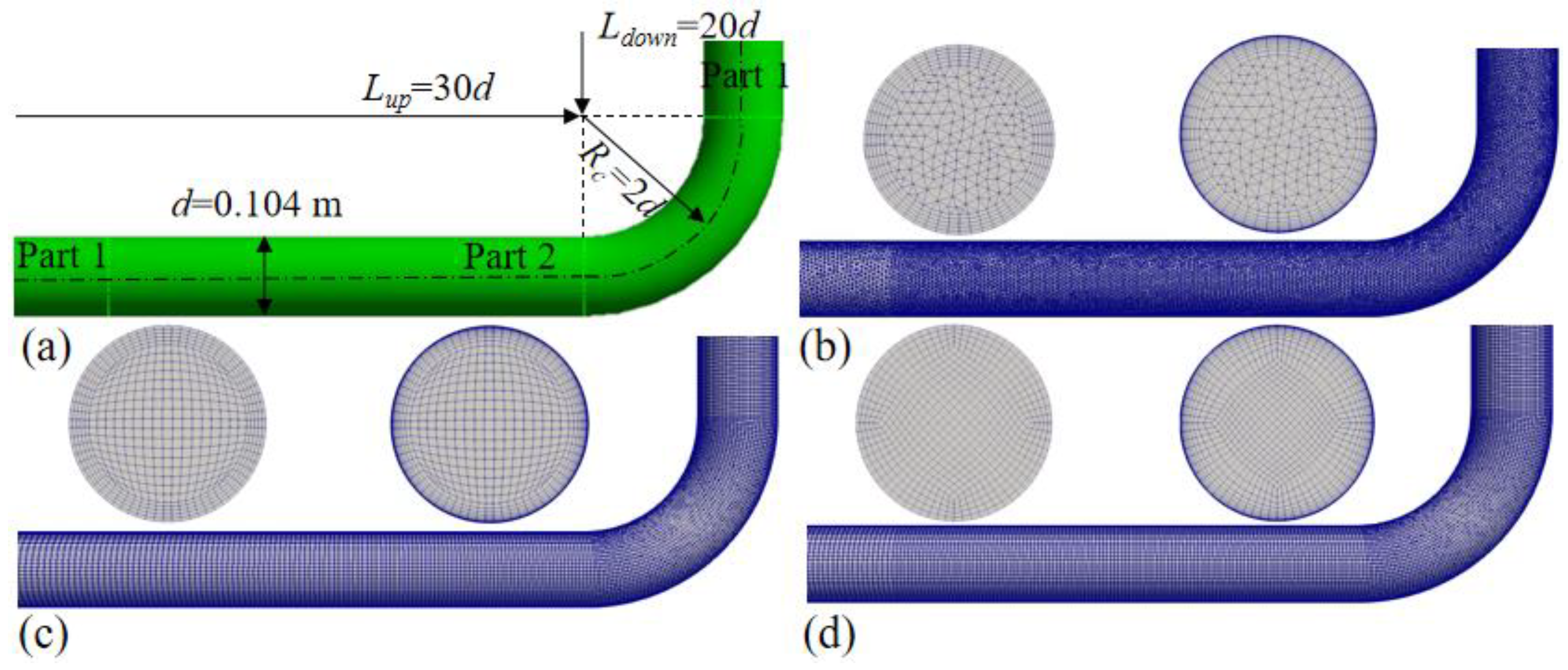
2.3. Computational Domain and Mesh

In this study, the experimental setup (Figure 1) for turbulent airflow through a 90° bend made by Sudo et al. [4] was used in simulations. The bend had an inner diameter d = 2R = 104 mm and a curvature radius of Rc = 208 mm. In this study, the computational domain was long enough to achieve a fully-developed flow condition, including a straight pipe in the upstream (30d), bend and a straight pipe in the downstream (20d). Two different meshes produced by ANSYS Workbench and one created by blockMesh were utilized to discretize the whole domain. Figure 2a shows the schematic of the straight pipe with a 90° bend. In the upstream and downstream mesh named in part one, a larger cell size than that of the bend (part 2) was used to decrease the total number of elements which in turn reduced the computational effort, as shown in Figure 2. Considering the influence of mesh and inflation layer on the flow field, the detailed sensitivity analysis of meshes was presented hereafter.

2.4. Boundary Conditions

Typically, three types of boundary conditions were required to be applied in pipe flow simulations. First, the uniform velocity, the turbulent kinetic energy, and the turbulent dissipation rate were prescribed at the pipe inlet (k = kin, ε = εin, U = 0, V = 0, and W = Win). At the pipe wall, the nonslip condition was imposed (U = V = W = 0). It should be noted that the log-law wall function had been applied for the high-Reynolds turbulence model while the boundary layer was fully resolved for capturing the viscous sublayer for the low-Reynolds turbulence model. Once the wall function was used, the dimensionless wall distance y+ from the first near-wall cell was strictly dropped in the range from 30 to about 130 in such a case, whereas a fully resolved boundary layer needs y+ of 1, according to the theory of channel flow. Finally, similar to references [35,36,37], the normal gradient of any variable has been considered as zero at the pipe outlet ( ψ / n = 0 ), except for a reference pressure value which was set as zero (relative pressure, Pr = 0).

3. Effect of Computational Mesh and Turbulence Modeling

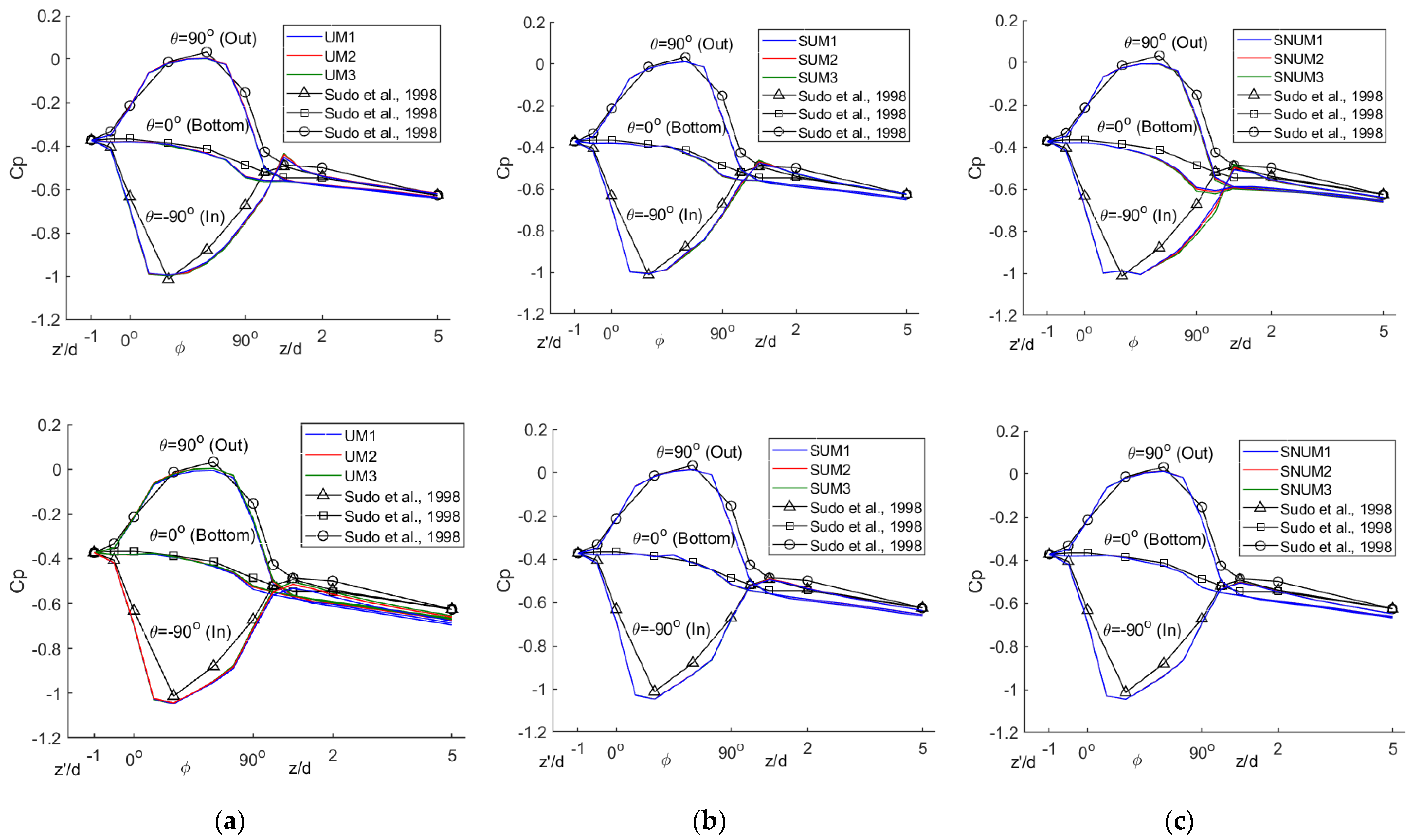
3.1. Parameters Used in Benchmarking

Here the preliminary study was obtained by numerically simulating the experiments of [4] since comprehensive measurements of turbulent flow through a bend with 90° have been made. The parameters used in their experiments were as follows: the bend had an inner diameter of d = 2R = 104 mm and a curvature radius of Rc = 208 mm, and the carrier fluid was air flowing (density ρ = 1.22 kg/m3 and kinematic viscosity ν = 1.46 × 10⁻⁵ m2/s) at a bulk-mean velocity of Win = 8.7 m/s. Therefore, the bulk Reynolds number was 6 × 10⁴, and the curvature ratio, Rc/d, was equal to two. The hot-wire anemometer technique was applied to measure the mean and fluctuating velocity fields in three directions, namely the longitudinal, circumferential, and radial directions. Reynolds stresses in several longitudinal cross-sections were also obtained. Additionally, the pressure coefficient, turbulent kinetic energy, secondary flow intensity, and primary flow deviation along the pipe were presented.

3.2. Types of Computational Meshes

As shown in Figure 2, the dimensionless distance from pipe wall y+ = 30 and y+ = 1 were both generated for three types of meshes, which depends on the choice of turbulence model. The standard k-ε turbulence model is accurate only if the first grid resides in the log-law region, here corresponding to y+ = 30. However, the low-Reynolds turbulence model, such as LaunderSharmaKE in OpenFOAM, requires a fully resolved boundary layer with y+ of 1. Note that a nonlinear eddy viscosity turbulence model such as LienCubicKE implemented in the current version of OpenFOAM is combined with its low-Reynolds and high-Reynolds models. Therefore, both meshes with y+ = 30 and y+ = 1 were used to test the mesh sensitivity. The inflation layer was applied to determine how the boundary layer was resolved. In terms of grid-independence analysis, the refinement of mesh was made by progressively reducing the cell size of two parts marked in Figure 2a. In the ANYSYS workbench, the body size tool was applied to define the cell size of those two parts for unstructured mesh and structured mesh with the nonuniform inflation layer while the number of divisions was modified in blockMesh for structured mesh with the analogous uniform inflation layer. All of the cases run in this study with detailed information related to mesh types, y+, cell number, and mesh quality, are listed in Table 4. To keep the similar inflation layer among the three types of meshes, only the body size of the core region was changed, and the inflation layer was kept at an unchanged number of layers and expansion ratio. It should be mentioned that only three meshes were tested for structured mesh with a uniform inflation layer for the reason that this type of mesh converged quickly with respect to the effect of grid size. Additionally, a nonuniformed mesh size was used for part one of this mesh type, thereby the total cell number is relatively smaller than that of the other structured type. But it is ensured that the grid size in part two, particularly near the bend, is nearly the same as other mesh types.

3.3. Grid Sensitivity Analysis

Among all cases, the pressure coefficient, turbulence kinetic energy (Equation (9)), and secondary flow magnitude (Equation (10)) along the pipe from upstream to downstream of the bend, axial velocity, in-plane velocity, and turbulence intensity at the cross-section of the bend exit were regarded as the identifier to verify if the solution reached grid-independent since those variables were used to characterize such a flow, according to a critical literature review. All variables were normalized by a factor according to Sudo et al. [4]. For the sake of brevity, only some representative results are presented in this paper. It should be noted that although some variables are shown in a qualitative manner, the results can still provide valuable information.
The grid convergence tests were carried out by considering three types of typical meshes, as illustrated in Table 4. UM1 to UM5, SUM1 to SUM3, and SNUM1 to SNUM5
k a = 4 π d 2 W i n 2 π / 2 π / 2 0 R 1 2 ( u 2 ¯ + v 2 ¯ + w 2 ¯ ) r d r d θ
I s = 4 π d 2 W i n 2 π / 2 π / 2 0 R 1 2 ( U 2 + V 2 ) r d r d θ
denote the different mesh sizes’ composition, ranging from coarse to fine for unstructured, structured with uniform inflation layer, and structured mesh with nonuniform mesh, respectively. During the grid refinement process, the total cell number was increased from coarse to fine grid as most researchers did. As anticipated, the turbulence models can lead to some differences among the results. Specifically, the converging rate changed with turbulence models for different mesh types. For instance, as shown in the top graph of Figure 3, all of the variables converged quickly, however, the turbulence kinetic energy attained convergence only in very fine meshes (UM5 and SNUM5), referring to the application of the nonlinear turbulence model with y+ of 30. Clearly, the secondary flow appears at the bend inlet, reaches the maximum value at the vicinity of the bend exit, and its magnitude starts to reduce rapidly. Similarly, the turbulence intensity begins to increase, arrives at its highest point in the vicinity of the bend exit, and then decreases. It is worth noting that there is no need to compare the numerical results with experimental data in the current stage (sensitivity analysis), aiming at exploring the effect of numerical and modeling factors on the numerical solutions while the validation of the model definitely requires it. The possible reason for the differences in the numerical results and experimental measurements could be the application of RANS-based turbulence modeling, which is incapable of accurately capturing the turbulence field in such a complex phenomenon, however, the predicted results should satisfy most of the engineering applications. Also, a similar observation was detected for the contour plot of turbulence intensity (Figure 4) when the standard k-ε turbulence model was used, however, this phenomenon only appeared in the unstructured mesh. Clearly, the largest local fluctuation (12%) appeared in the region near the inner wall due to the steep velocity gradient (Figure 5) along with the depression of the mean velocity, whereas a relatively weak fluctuation happened to the outer wall since the velocity gradient there was gentle. However, as demonstrated in Figure 5, the mean axial velocity at the bend exit was slightly sensitive to the mesh sizes, whereas the changes in the other variables were negligible. It should be mentioned that the left-hand side was the inner wall of the bend while the right represented the outer wall in all of the contour and vector plots in this study. Obviously, the tongue-shaped velocity distribution appeared due to the remarkable distortion of primary fluid induced by the secondary flow near the bend exit. It could be also detected from the three-dimensional flow structure by streamlining, as shown in Figure 6. It was clear that the convergence rate was not significantly affected by the mesh sizes once the boundary layer was fully resolved, corresponding to y+ of 1. UM3, SUM3, and SNUM3 were fine enough to get a grid-independent solution for all turbulence models considered in this work, which was probably a consequence of a more accurate solution obtained from the resolved boundary layer than that with the usage of the wall function.
In terms of other variables, such as pressure coefficients (Cp = (PaPref)/0.5ρWin2), indicating the difference of wall static pressure in various locations and a reference point in the upstream (z = −17.6d) divided by 0.5ρWin2 and the velocity vector of the secondary flow at bend exit are demonstrated in Figure 7 and Figure 8, respectively. For the sake of space, the results for those two variables calculated by the nonlinear turbulence model were taken as an example. As for the pressure coefficients (Figure 7), overall, no difference was observed, neither from the different mesh sizes nor the mesh types. However, the pressure drop predicted by two structured meshes was slightly larger than that of unstructured mesh. Additionally, all pressure drop calculated by the low-Reynolds turbulence model was larger than that of the high-Reynolds models. This is also true for the nonlinear turbulence model with y+ of 1. Due to the insensitivity to mesh sizes, a secondary velocity vector was only presented for the finest mesh. Obviously, all of the mesh types could capture well the Dean vortex (Figure 8) which should be a pair of counter-rotating vortices caused by the symmetric pipe. Usually, the secondary flow induced by the centrifugal force occurs in the cross section of the bend starting from φ = 30° and the Dean vortex circulates outwards in the center part of the pipe and inwards near the upper and lower walls [20]. Not surprisingly, the Dean vortex predicted by SNUM5 was relatively weaker especially in the four corners near the inflation layer due to the certain skewness in this region. This difference can be neglected.
The types of meshes still have some influence on the turbulence intensity when a nonlinear turbulence model with a wall function (y+ = 30) was applied. Figure 9 demonstrates the turbulence intensity at the bend exit for the three types of meshes. Again, the variable shown here is grid independent. It was obvious that a large deviation happens to the inner wall of the bend among the different mesh types. A relatively larger gradient of turbulence intensity was captured by UM5 and SNUM5, and a wide range of larger isolines was found in the simulation SNUM5. This phenomenon was consistent with the average turbulence kinetic energy illustrated in Figure 3, in the sense that the average turbulence kinetic energy of the cross-section for SNUM5 was larger than that of the other two meshes. It was also found that the variable was almost the same between SUM3 and UM5 due to the wide range of larger isolines in SUM3, although there was no strong gradient of turbulence kinetic energy detected. This was also true for the effect of mesh types on the axial velocity at the bend exit, as demonstrated in Figure 10. As can be seen from Figure 11, the shape of the isolines near the inner wall predicted by SNUM5 was different from the other two to some degree. There were also some spurious types of mesh effects with the standard k-ε model, however, this is more moderate.
Surprisingly, as can be seen from Figure 9, the performance of a nonlinear turbulence model with a fully resolved boundary layer (y+ = 1) was not improved as expected, regarding the turbulence intensity. Its peak value was lower than that obtained from the model with the application of the wall function and no large gradient occurred near the inner wall. So far, the reason for this observation is still not yet clear.
It is accepted that the adoption of a log-law wall function ranged from y+ of 30 to 300, more or less. Given that, y+ of 40 and 50 were also considered in this study to confirm whether the observations detected above will be changed with a different y+. Here, only the predictions of turbulence intensity made by structured mesh with a uniform inflation layer and a nonlinear turbulence model with y+ of 40 and 50 are presented (Figure 11). The results demonstrated that the same rule was also suitable for the larger y+ than 30.

3.4. Considerations of Computational Effort

The mesh had a significant influence on the stability and convergence of CFD modelling, thereby probably affecting the accuracy of the solutions. As described in Table 4, two peculiarities were used to evaluate the quality of meshes, namely average nonorthogonality and maximum skewness. It seems that SUM and UM meshes are nonorthogonal to a large extent and they have a lower skewness, compared with SNUM. The value was nearly double for average nonorthogonality. However, the overall mesh quality of all of the meshes used here was fairly satisfactory without confronting any convergence issues during calculation. Consequently, the effect of mesh quality can be neglected in this work.
In terms of computational effort, of course, many more cells were required for unstructured mesh, in comparison with structured mesh. Obviously, the total number of unstructured mesh was more or less five times that of structured mesh. Therefore, the calculation time of the unstructured mesh needed was rather longer than the structured mesh. Even though the half geometry of the pipe bend allows it to be used, the computational effort was still huge, aiming at getting grid-independent solutions.

3.5. Influence of Curvature Ratio and Reynolds Number

The curvature ratio and Reynolds number are the crucial parameters for turbulent pipe bend flow. As is known, a longer bend and a larger Reynolds number can alleviate the effect of bend in general. Furthermore, this influence induced by the curvature ratio was much stronger than the Reynolds number. In order to get rid of the effects of the Reynolds number and the curvature ratio, another two curvature ratios (Rc/d = 1 and Rc/d = 3) and the Reynolds number (Re = 35,616 and Re = 88,328) were chosen for conducting the mesh sensitivity analysis. As expected, it was found that the rule is also valid for these situations no matter what the values of curvature ratio and Reynolds number were. Again, only the turbulence intensity contour at the bend exit for the nonlinear turbulence model and the unstructured mesh with a uniform inflation layer is presented. As illustrated in Figure 12, the large gradient can be also observed near the inner wall when y+ is equal to one due to the large adverse pressure gradient and flow separation. However, the peak value for y+ of 30 was also larger than that of y+ of 1, which was consistent with the previous predictions. The turbulence intensity for a longer bend regarding the different boundary layer treatments is depicted in Figure 13. Clearly, the turbulence intensity decreased significantly with the increases in curvature ratio since the bend effect was relatively weak. As shown in Figure 14 and Figure 15, the large peak value and gradient of turbulence intensity in the vicinity of the inner wall were only captured by the model with the wall function used. Of course, a much larger turbulence intensity appeared in the condition of higher Re than that of the lower one.

4. Conclusions

In this study, RANS-based simulations of the turbulent flow in pipe bends were performed using the OpenFOAM code. The experiment of Sudo et al. [4] was simulated to investigate how the CFD solution was affected by computational mesh type and near-wall mesh resolution, as well as the turbulence model. Three kinds of meshes and turbulence models were taken into account in CFD modelling. Based on the current investigations, the following preliminary conclusions could be drawn:
(1)
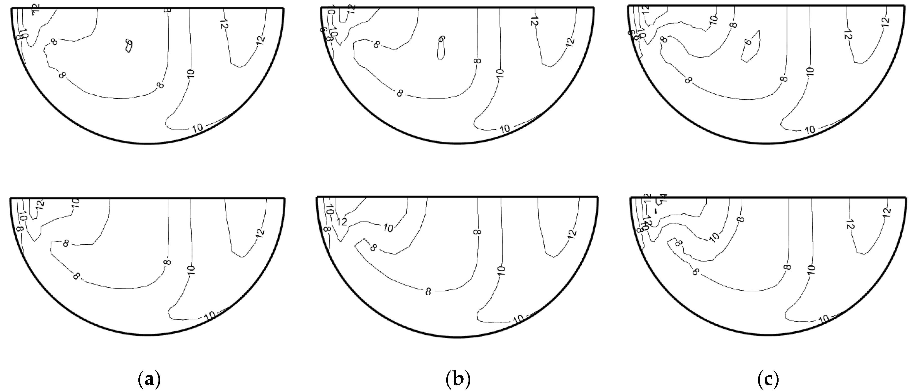
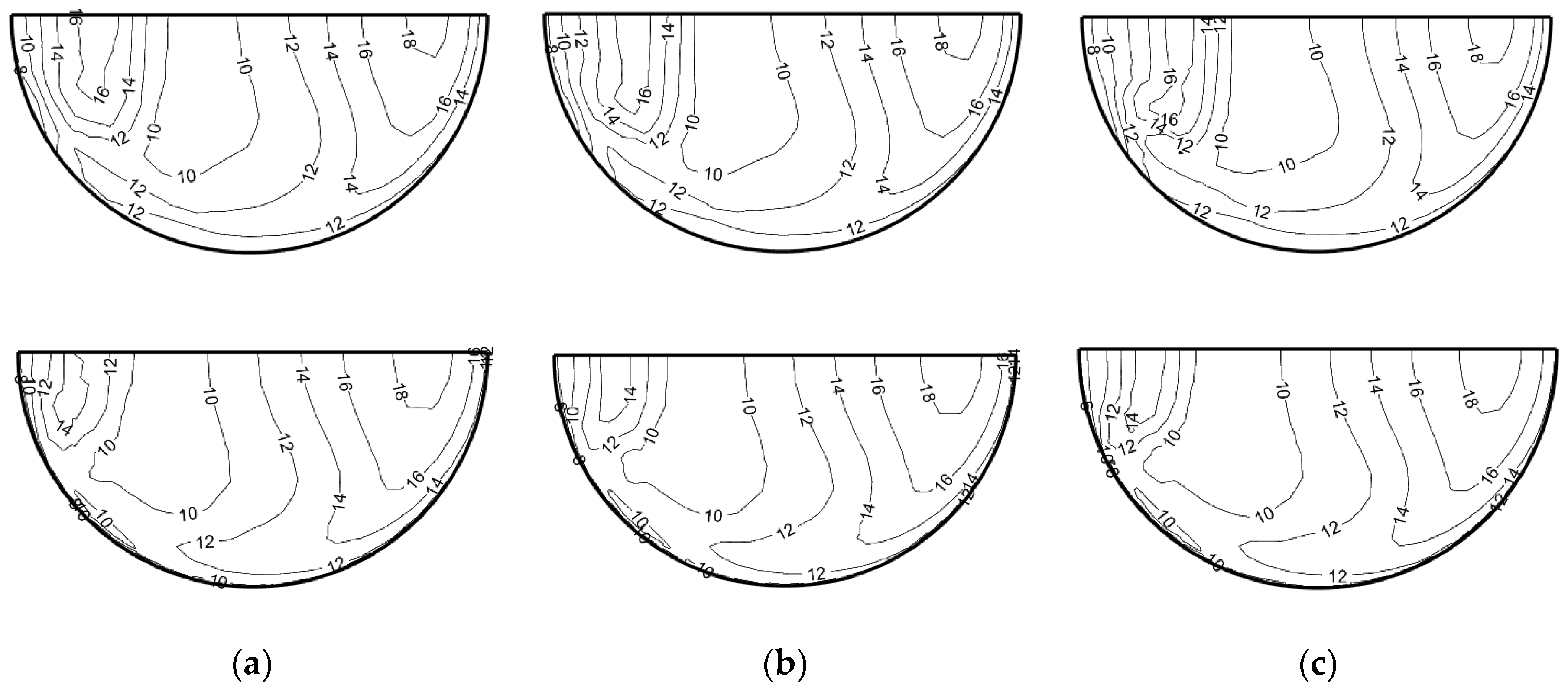
Computational mesh has a certain impact on those critical variables concerned in this study. The most sensitive variable regarding turbulent pipe bend flow was turbulent kinetic energy. The sensitivity of the turbulence intensity to mesh sizes also relies on the application of the turbulence model (Figure 3 and Figure 4). The sensitivity of mesh sizes on the turbulence kinetic energy can be reduced, provided that the boundary layer is fully resolved, especially for the configurations where the turbulence model based on the nonlinear eddy viscosity hypothesis is utilized, combined with unstructured mesh and structured mesh with a nonuniform inflation layer.
(2)
In contrast, other variables, such as pressure coefficient (Figure 7), secondary flow velocity, and its intensity (Figure 3) tend to be stable with the refinement of computational mesh, regardless of a slight change of axial velocity with mesh sizes (Figure 5).
(3)
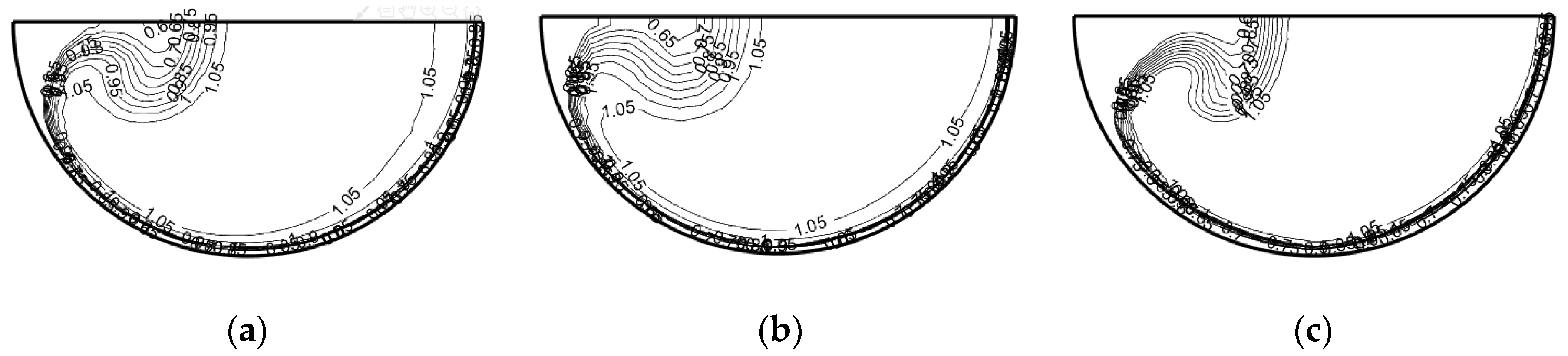
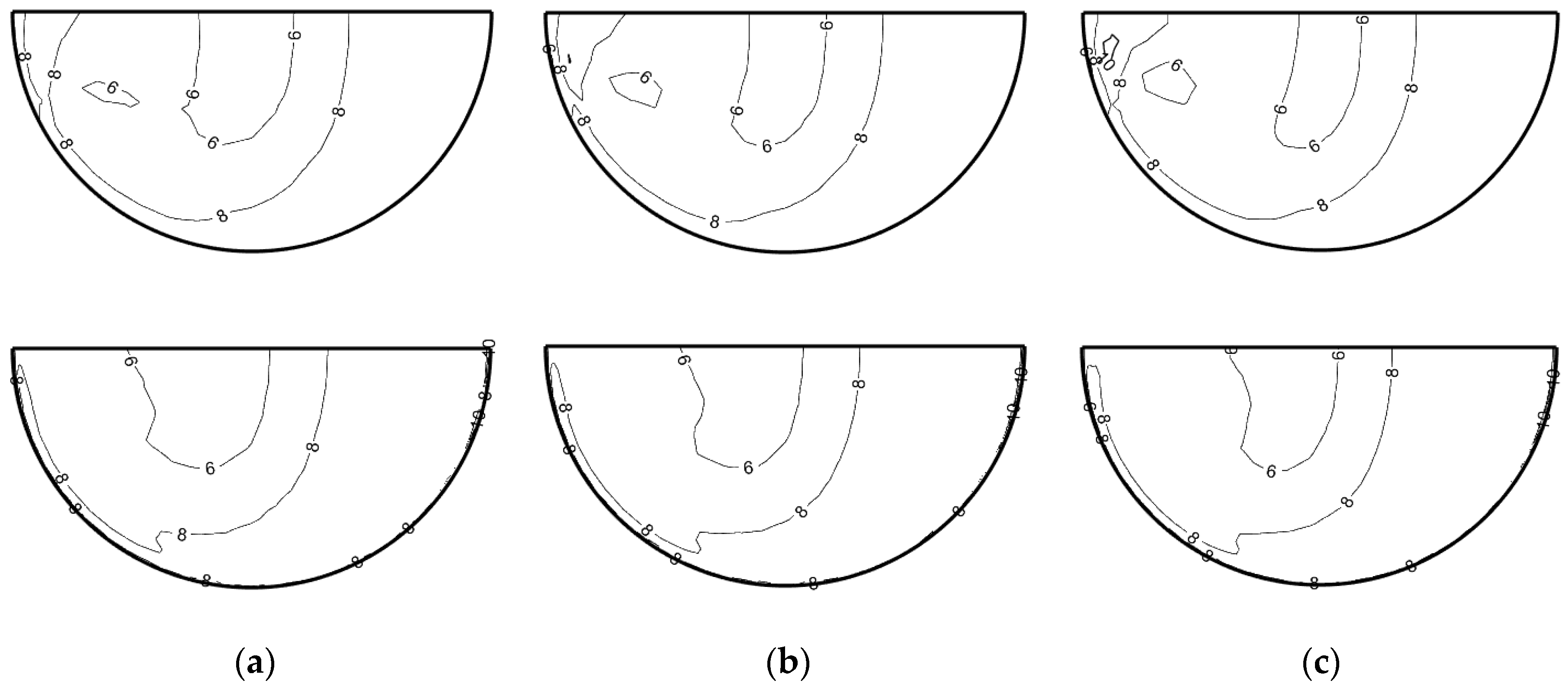
The influence of mesh types on turbulence intensity is remarkable (Figure 9), as the smaller peak value and the gradient close to the near wall were captured by structured mesh with a uniform inflation layer when it comes to y+ of 30, compared with another two meshes. However, the fully resolved boundary layer seemed not to improve the results since the gradient and peak value near the inner wall had not been detected. The reason for this will be investigated in future work.
(4)
Contrarily, the pressure coefficient (Figure 7), secondary flow velocity vector (Figure 8), and its intensity (Figure 3) remained unchanged no matter which mesh type was applied, regardless of visible change in axial velocity with mesh sizes (Figure 10).
(5)
The same rule was still true for the different y+ (Figure 11), curvature ratios (Figure 12 and Figure 13), and Reynolds numbers (Figure 14 and Figure 15). Even though the flow separation occurred in a sharp bend, a similar phenomenon was observed.
Altogether, a recommendation for the computational mesh of turbulent flow through pipe bends could be a structured mesh associated with uniform inflation layers. These findings pave the way for further exploring the hydrate slurry flow in a pipe bend.

Author Contributions

Conceptualization, Q.Y. and P.Y.; formal analysis, T.X. and Y.Z.; data curation, Y.G. and Y.T.; writing—original draft preparation, P.Y. and J.D.; writing—review and editing, Q.Y. and P.Y.; visualization, Y.G. and T.X.; project administration, J.D.; funding acquisition, X.L. and Q.Y. The final manuscript has been approved by all the authors. All authors have read and agreed to the published version of the manuscript.

Funding

This work is financially sponsored by the China Scholarship Council (CSC), supported by the National Natural Science Foundation of China (Grant No. 41572247, 42077237) and the Natural Science Foundation of Shandong Province (Grant No. ZR2020MD110). Technical assistance from Prof. G.V. Messa and Prof. S. Malavasi of Politecnico di Milano is greatly appreciated.

Institutional Review Board Statement

Not applicable.

Informed Consent Statement

Not applicable.

Data Availability Statement

The data presented in this study are available on request from the corresponding author.

Conflicts of Interest

The authors declare no conflict of interest.

Nomenclature

i: j, kindices of structured grid
z, zlongitudinal distance along the pipe axis
θ, razimuthal coordinate and radial coordinate
dpipe diameter
Rpipe radius
Rccurvature radius of pipe bend
φangle from the bend inlet
Lup, Ldownlength of upstream and downstream straight pipe
U, V, Wtime-averaged velocity in three directions
u’, v’, wfluctuating velocity in three directions
kturbulent kinetic energy (TKE)
ε, ε ˜ dissipation rate of TKE
Pkproduction of TKE
ρdensity of fluid
νkinetic viscosity of the fluid
νtturbulent viscosity of the fluid
C ε 1 , C ε 2 , σ k , σ ε coefficients in the turbulence model
f1, f2, Edamping coefficients and source term in the turbulence model
Win, kin, ε in velocity, TKE, and dissipation rate of TKE at the inlet
ggravitational acceleration
ReReynolds number
Pastatic pressure at any position
Prefreference value of Pa
Prrelative air pressure
ψ general variable
nnormal vector of cell surface
Cppressure coefficient, Cp = (Pa-Pref)/(ρWin2/2)
Issecondary flow intensity
katurbulence intensity

References

  1. He, X.L.; Sourabh, V.A.; Shashank, K.K.; Ömer, N.D. An LES study of secondary motion and wall shear stresses in a pipe bend. Phys. Fluids 2021, 33, 115102. [Google Scholar] [CrossRef]
  2. Wegt, S.; Maduta, R.; Kissing, J.; Hussong, J.; Jakirlić, S. LES-based vortical flow characterization in a 90°-turned pipe bend. Comput. Fluids 2022, 240, 105418. [Google Scholar] [CrossRef]
  3. Dean, W.R. Note on the motion of fluid in a curved pipe. Philos. Mag. 1927, 4, 208–223. [Google Scholar] [CrossRef]
  4. Sudo, K.; Sumida, H.; Hibara, H. Experimental investigation on turbulent flow in a circular-sectioned 90-degree bend. Exp. Fluids 1998, 25, 42–49. [Google Scholar] [CrossRef]
  5. Weske, J.R. Experimental Investigation of Velocity Distributions Downstream of Single Duct Bends; Report No. NACA-TN-1471; National Advisory Committee for Aeronautics: Boston, MA, USA, 1948. [Google Scholar]
  6. Hellström, L.H.O.; Sinha, A.; Smits, A.J. Visualizing the Very-Large-Scale motions in turbulent pipe flow. Phys. Fluids 2011, 23, 011703. [Google Scholar] [CrossRef]
  7. Vester, A.K.; Örlü, R.; Alfredsson, P.H. Turbulent flows in curved pipes: Recent advances in experiments and simulations. Appl. Mech. Rev. 2016, 68, 050802. [Google Scholar] [CrossRef]
  8. Weisbach, J. Experimentelle Hydraulik; Engelhardt: Freiberg, Germany, 1855. [Google Scholar]
  9. Thomson, J. On the origin of windings of rivers in alluvial plains with remarks on the flow of water round bends in pipes. Proc. R. Soc. Lond. 1876, 25, 5–8. [Google Scholar]
  10. Thomson, J. Experimental demonstration in respect to the origin of windings of rivers in alluvial plains, and to the mode of flow of water round bends of pipes. Proc. R. Soc. Lond. 1877, 26, 356–357. [Google Scholar]
  11. Williams, G.S.; Hubbell, C.W.; Fenkell, G.H. Experiments at Detroit, MI, on the Effect of curvature upon the flow of water in pipes. Trans. Am. Soc. Civ. Eng. 1902, 47, 1–196. [Google Scholar] [CrossRef]
  12. Eustice, J. Flow of water in curved pipes. Proc. R. Soc. Lond. 1910, 84, 107–118. [Google Scholar]
  13. Eustice, J. Experiments on stream-line motion in curved pipes. Proc. R. Soc. Lond. 1911, 85, 119–131. [Google Scholar]
  14. Dean, W.R. The stream-line motion of fluid in a curved pipe. Philos. Mag. 1928, 5, 671–695. [Google Scholar] [CrossRef]
  15. Adler, M. Strömung in gekrümmten Rohren. J. Appl. Math. Mech. Z. Angew. Math. Mech. 1934, 14, 257–275. [Google Scholar] [CrossRef]
  16. Rowe, M. Measurements and computations of flow in pipes. J. Fluid Mech. 1998, 43, 771–783. [Google Scholar] [CrossRef] [Green Version]
  17. Anwer, M.; So, R.M.C.; Lai, Y.G. Perturbation by and recovery from bend curvature of a fully developed turbulent pipe flow. Phys. Fluids A Fluid Dyn. 1989, 1, 1387. [Google Scholar] [CrossRef]
  18. Enayet, M.M.; Gibson, M.M.; Taylor, A.M.K.P.; Yianneskis, M. Laser Doppler measurements of laminar and turbulent flow in a pipe bend. Int. J. Heat Fluid Flow 1982, 3, 213–219. [Google Scholar] [CrossRef]
  19. Azzola, J.; Humprey, J.A.C.; Iacovides, H.; Launder, B.E. Developing turbulent flow in a U-bend of circular cross-section: Measurement and computation. ASME J. Fluids Eng. 1986, 108, 214–221. [Google Scholar] [CrossRef]
  20. Patankar, S.V.; Pratap, V.S.; Spalding, D.B. Prediction of turbulent flow in curved pipes. J. Fluid Mech. 1975, 67, 583–595. [Google Scholar] [CrossRef]
  21. Rowe, M. Some Secondary Flow Problems in Fluid Dynamics. Ph.D. Thesis, Cambridge University, Cambridge, UK, 1966. [Google Scholar]
  22. Al-Rafai, W.N.; Tridimas, Y.D.; Woolley, N.H. A study of turbulent flows in pipe bends. Proc. Inst. Mech. Eng. Part C J. Mech. Eng. Sci. 1990, 204, 399–408. [Google Scholar] [CrossRef]
  23. Lai, Y.; So, R.M.C.; Zhang, H.S. Turbulence-driven secondary flows in a curved pipe. Theor. Comput. Fluid Dyn. 1991, 3, 163–180. [Google Scholar] [CrossRef]
  24. Wang, J.R.; Shirazi, S.A. A CFD based correlation for mass transfer coefficient in elbows. Int. J. Heat Mass Transf. 2001, 44, 1817–1822. [Google Scholar] [CrossRef]
  25. Pruvost, J.; Legrand, J.; Legentilhomme, P. Numerical investigation of bend and torus flows—Part I: Effect of swirl motion on flow structure in U-bend. Chem. Eng. Sci. 2004, 59, 3345–3357. [Google Scholar] [CrossRef]
  26. Hilgenstock, A.; Ernst, R. Analysis of installation effects by means of Computational Fluid Dynamics—CFD versus experiments? Flow Meas. Instrum. 1996, 7, 161–171. [Google Scholar] [CrossRef]
  27. Kim, J.; Yadav, M.; Kim, S. Characteristics of secondary flow induced by 90-degree elbow in turbulent pipe flow. Eng. Appl. Comput. Fluid Mech. 2014, 8, 229–239. [Google Scholar] [CrossRef] [Green Version]
  28. Wang, L.W.; Gao, D.R.; Zhang, Y.G. Numerical simulation of turbulent flow of hydraulic oil through 90° circular-sectional bend. Chin. J. Mech. Eng. 2012, 25, 905–910. (In Chinese) [Google Scholar] [CrossRef]
  29. Chen, M.; Zhang, Z.G. Numerical simulation of turbulent driven secondary flow in a 90° bend pipe. Adv. Mater. Res. 2013, 765–767, 514–519. [Google Scholar] [CrossRef]
  30. Dutta, P.; Saha, S.K.; Nandi, N. Numerical study on flow separation in 90° pipe bend under high Reynolds number by k-ε modelling. Eng. Sci. Technol. Int. J. 2016, 19, 904–910. [Google Scholar] [CrossRef]
  31. Hossain, S.; Hossain, I. Computational investigation of turbulent flow development in 180° channel with circular cross section. Eur. J. Eng. Res. Sci. 2018, 3, 98–105. [Google Scholar] [CrossRef]
  32. Dutta, P.; Saha, S.K.; Nandi, N. Numerical study of curvature effect of turbulent flow in 90° pipe bend. In Proceedings of the ICTACEM 2014 International Conference on Theoretical, Applied, Computational and Experimental Mechanics, IIT, Kharagpur, India, 29–31 December 2014. [Google Scholar]
  33. Chowdhury, R.R.; Alam, M.M.; Sadrul Islam, A.K.M. Numerical modeling of turbulent flow through bend pipes. Mech. Eng. Res. J. 2016, 10, 14–19. [Google Scholar]
  34. Ayala, M.; Cimbala, J.M. Numerical approach for prediction of turbulent flow resistance coefficient of 90° pipe bends. Proc. Inst. Mech. Eng. Part E J. Process Mech. Eng. 2020, 235, 351–360. [Google Scholar] [CrossRef]
  35. Jurga, A.P.; Janocha, M.J.; Yin, G.; Ong, M.C. Numerical simulations of turbulent flow through a 90-deg pipe bend. J. Offshore Mech. Arct. Eng. 2022, 144, 061801. [Google Scholar] [CrossRef]
  36. Zhang, J.; Wang, D.; Wang, W.; Zhu, Z. Numerical investigation and optimization of the flow characteristics of bend pipe with different bending angles. Processes 2022, 10, 1510. [Google Scholar] [CrossRef]
  37. Yin, G.; Ong, M.C.; Zhang, P.Y. Numerical investigations of pipe flow downstream a flow conditioner with bundle of tubes. Eng. Appl. Comput. Fluid Mech. 2023, 17, e2154850. [Google Scholar] [CrossRef]
  38. Launder, B.E.; Spalding, D.B. The numerical computation of turbulent flows. Comput. Methods Appl. Mech. Eng. 1974, 3, 269–289. [Google Scholar] [CrossRef]
  39. Launder, B.E.; Sharma, B.I. Application of the energy-dissipation model of turbulence to the calculation of flow near a spinning disc. Lett. Heat Mass Transf. 1974, 1, 131–137. [Google Scholar] [CrossRef]
  40. Lien, F.S.; Chen, W.L.; Leschziner, M.A. Low-Reynolds-number eddy-viscosity modeling based on non-linear stress-strain/vorticity relations. Eng. Turbul. Model. Exp. 1996, 3, 91–100. [Google Scholar]
Figure 1. Schematic diagram of the test pipe and coordinate system used in Sudo et al. [4].
Jmse 11 00336 g001
Figure 2. Pipe bend geometry and corresponding meshes: (a) Schematic of pipe bend used in simulations; (b) Unstructured mesh; (c) Structured mesh with uniform inflation layer; (d) Structured mesh with nonuniform inflation layer.
Jmse 11 00336 g002
Figure 3. The longitudinal distribution of the average magnitude of secondary flow and turbulent kinetic energy along the pipe regarding a nonlinear eddy viscosity turbulence model: top and bottom rows are y+ = 30 and y+ = 1, respectively: (a) UM; (b) SUM; (c) SNUM [4].
Jmse 11 00336 g003
Figure 4. Turbulence intensity at bend exit regarding standard k-ε turbulence model: (a) UM1; (b) UM2; (c) UM3; (d) UM4; (e) UM5.
Jmse 11 00336 g004
Figure 5. Axial velocity at bend exit regarding standard k-ε turbulence model: (a) UM1; (b) UM2; (c) UM3; (d) UM4; (e) UM5.
Jmse 11 00336 g005
Figure 6. The schematic view of 3D flow structure by streamline.
Jmse 11 00336 g006
Figure 7. Longitudinal distribution of pressure coefficient: top and bottom rows are nonlinear turbulence model with y+ of 30 and low-Reynolds turbulence model, respectively: (a) UM; (b) SUM; (c) SNUM [4].
Jmse 11 00336 g007
Figure 8. Secondary velocity vector regarding nonlinear eddy viscosity turbulence model: (a) UM5; (b) SUM3; (c) SNUM5.
Jmse 11 00336 g008
Figure 9. Turbulence intensity at bend exit regarding nonlinear eddy viscosity turbulence model: top and bottom rows are y+ = 30 and y+ = 1, respectively: (a) UM5; (b) SUM3; (c) SNUM5.
Jmse 11 00336 g009
Figure 10. Axial velocity at bend exit regarding nonlinear eddy viscosity turbulence model with y+ of 30: (a) UM5; (b) SUM3; (c) SNUM5.
Jmse 11 00336 g010
Figure 11. Turbulence intensity at bend exit regarding nonlinear eddy viscosity turbulence model: top and bottom rows are y+ = 40 and y+ = 50, respectively: (a) SUM1; (b) SUM2; (c) SUM3.
Jmse 11 00336 g011
Figure 12. Turbulence intensity at bend exit regarding nonlinear eddy viscosity turbulence model for Rc/d = 1: top and bottom rows are y+ = 30 and y+ = 1, respectively: (a) SUM1; (b) SUM2; (c) SUM3.
Jmse 11 00336 g012
Figure 13. Turbulence intensity at bend exit regarding nonlinear eddy viscosity turbulence model for Rc/d = 3: top and bottom rows are y+ = 30 and y+ = 1, respectively: (a) SUM1; (b) SUM2; (c) SUM3.
Jmse 11 00336 g013
Figure 14. Turbulence intensity at bend exit regarding nonlinear eddy viscosity turbulence model for Re = 35,616: top and bottom rows are y+ = 30 and y+ = 1, respectively: (a) SUM1; (b) SUM2; (c) SUM3.
Jmse 11 00336 g014
Figure 15. Turbulence intensity at bend exit regarding nonlinear eddy viscosity turbulence model for Re = 88,328: top and bottom rows are y+ = 30 and y+ = 1, respectively: (a) SUM1; (b) SUM2; (c) SUM3.
Jmse 11 00336 g015
Table 1. Related terms and coefficient in standard k-ε turbulence model.
u i u j ¯ / k ν t P k S S i j
2 3 δ i j ν t k S i j C μ k 2 ε ν t S 2 2 S i j S i j 1 2 ( U i , j + U j , i )
C ε 1 C ε 2 C μ σ k σ ε
1.441.920.0911.3
Table 2. Related terms and coefficient in low-Reynolds k-ε turbulence model.
ν t   ε ˜ D E f μ   f 1  
C μ f μ k 2 ε ˜ ε D 2 ν ( k x i ) 2 2 ν ν t ( 2 U i x i x k ) 2 e 3.4 ( 1 + R T / 50 ) 2 1 
f 2 R T C ε 1 C ε 2 C μ σ k σ ε
1 0.3 e R T 2 k 2 ν ε ˜ 1.440.920.0911.22
Table 3. Related terms and coefficient in LienCubicKE turbulence model.
ν t   f μ   f 1   f 2   y *   R T   P k  
C μ f μ k 2 ε ( 1 e 0.198 y * ) ( 1 + 5.29 y * ) 1 + P k P k 1 0.3 e R T 2 y k / ν k 2 ν ε 1.33 ( 1 0.3 e R T 2 ) ( 1 + 2 ν k y 2 ) e 0.00375 y * 2
u i u j ¯ / k
2 3 δ i j ν t k S i j + C 1 ν t ε ( S i k S k j 1 3 δ i j S k l S k l ) + C 2 ν t ε ( Ω i k S k j + Ω j k S k i ) + C 3 ν t ε ( Ω i k Ω j k 1 3 δ i j Ω l k Ω l k ) + C 4 ν t k ε 2 ( S k i Ω l j + S k j Ω l i ) S k l + C 5 ν t k ε 2 ( S k l S k l Ω k l Ω k l ) S i j
C μ C 1 C 2 C 3 C 4 C 5 S Ω Ω i j
2 / 3 1.25 + S + 0.9 Ω 3 / 4 1000 + S 3 15 / 4 1000 + S 3 19 / 4 1000 + S 3 10 C μ 2 2 C μ 2 k ε 1 2 S i j S i j k ε 1 2 Ω i j Ω i j 1 2 [ U i , j U j , i ]
Table 4. The details of computational meshes used in this study.
Mesh TypesAbbreviationThe Cell Size of Part 1 (m)The Cell Size of Part 2 (m)Number of Inflation LayerGrowth Ratio of Inflation LayerTotal Cells NumberAverage NonorthogonalityMax Skewness
y+ = 30y+ = 1y+ = 30y+ = 1y+ = 30y+ = 1y+ = 30y+ = 1y+ = 30y+ = 1
Unstructured meshUM10.00950.0075141.051.325713,1351,260,91112.469.540.7450.756
UM20.0080.0061,093,0091,843,73612.749.830.7360.791
UM30.00650.0051,843,1342,935,31912.9910.220.8620.780
UM40.00550.0043,054,005-13.19-0.803-
UM50.0040.0035,066,295-13.59-0.843-
Structured mesh with uniform inflation layerSUM10.00950.007163,584347,61612.919.430.5290.577
SUM20.0080.006241,808497,84013.389.670.5940.64
SUM30.00650.005377,400744,60013.9810.130.670.711
Structured mesh with nonuniform inflation layerSNUM10.00950.007246,144553,8245.814.421.1750.601
SNUM20.0080.006360,808785,2885.984.591.0200.630
SNUM30.00650.005579,3091,205,5896.204.810.8370.715
SNUM40.00550.004953,988-6.43-0.670-
SNUM50.0040.0031,761,984-6.69-0.605-
Disclaimer/Publisher’s Note: The statements, opinions and data contained in all publications are solely those of the individual author(s) and contributor(s) and not of MDPI and/or the editor(s). MDPI and/or the editor(s) disclaim responsibility for any injury to people or property resulting from any ideas, methods, instructions or products referred to in the content.

