
Reynolds-Averaged Simulation of Drag Reduction in Viscoelastic Pipe Flow with a Fixed Mass Flow Rate

School of Marine Science and Technology, Northwestern Polytechnical University, Xi’an 710072, China
*
Author to whom correspondence should be addressed.
J. Mar. Sci. Eng. 2023, 11(4), 685; https://doi.org/10.3390/jmse11040685
Submission received: 7 February 2023
/
Revised: 1 March 2023
/
Accepted: 14 March 2023
/
Published: 23 March 2023
(This article belongs to the Special Issue Computational Fluid Mechanics II)
Abstract
:A high molecular polymer solution with viscoelasticity has the effect of reducing frictional drag, which is quite practical for energy saving. Effective simulations of viscoelastic flows in a pipeline with a high Reynolds number is realized by incorporating the constitutive equation of viscoelasticity into the
turbulence model. The Finitely Extensive Nonlinear Elastic Peterlin (FENE-P) model is employed for characterizing the viscoelasticity. The drag reduction of fully developed viscoelastic pipe flow with a fixed mass flow rate is studied. Different from increasing the center velocity and without changing the velocity near the wall at a fixed pressure drop rate, the addition of a polymer reduces the velocity near the wall and increases the velocity at the center of the pipe and makes the flow tend to be a laminar flow. Decreasing the solvent viscosity ratio or increasing the maximum extensibility or the Weissenberg number can effectively reduce the turbulence intensity and the wall friction. Under the premise of ensuring calculation accuracy, this Reynolds-averaged simulation method for viscoelastic flow has significant advantages in both computational cost and accuracy, which is promising for drag reduction simulation and practical engineering applications.
1. Introduction
High molecular weight polymers have been found to be able to significantly reduce frictional resistance [1,2]. Polymer drag reduction (DR) has prospects for wide applications in practical engineering, such as the energy saving of water vehicles, the transportation efficiency of pipelines, etc. Polymers have been proven to be able to achieve a more than 80% DR rate [3,4].
The properties of viscoelastic fluid have been studied experimentally. The first comprehensive experimental study of the DR flow in a pipeline was carried out by Virk [5], who also put forward the maximum drag reduction asymptote (MDRA). Ptasinski [6] used laser Doppler velocimetry (LDV) for flow measurements of a polymer-containing drag-reducing fluid in a pipeline. They measured the magnitude of the flow shear stress and concluded that the polymer additives caused the drop of the Reynolds shear stress.
However, experimental studies have failed to obtain key information about the DR mechanism of viscoelastic fluid, such as the molecular conformation tensor [7]. Tsukahara et al. [8] studied turbulent drag reduction in a channel. In the near-wall region, the positive work of viscoelastic stress is closely related to the vortex stretching that generates turbulent kinetic energy from the stored elastic energy.
Therefore, many scholars have explored the DR of viscoelastic fluid using numerical simulations. Commonly used models for the viscoelastic fluid include the Finitely Extensive Nonlinear Elastic Peterlin (FENE-P) model, the Oldroyd-B model, and the Giesekus model, where the first model (FENE-P) is the most developed. At present, it is generally believed that the DR mechanism of polymers is to induce the conversion of turbulent energy into elastic energy. Those molecules stretch near the wall, including the buffer layer and the viscous sublayer, resulting in the DR effects of polymer additives. Sureshkumar et al. [9] performed simulations of fully developed flow with viscoelasticity and successfully reproduced the decrease in Reynolds stress and the expansion of the buffer layer, which were observed experimentally. Angelis et al. [10] studied near-wall viscoelastic flow with the FENE-P model. They found that the polymer molecules were stretched by the flow. The above works have provided an important foundation for understanding the acting mechanism of viscoelastic fluid [11,12]. Pereira et al. [13] analyzed the stretching mechanism of a polymer coil in turbulent drag reduction flow by direct numerical simulation.
The above-mentioned works used direct numerical simulation (DNS) to simulate viscoelastic fluid. However, the extremely complex nature of turbulence means that DNS imposes huge demands on computing resources. In contrast to DNS, the Reynolds-averaged Navier–Stokes (RANS) approach can simulate high Reynolds number turbulent flow with both acceptable accuracy and computational efficiency. A basis for the RANS simulation of a viscoelastic flow was established by Leighton [14], who put forward a viscoelastic DR model with a Reynolds average of the constitutive equation of the FENE-P viscoelasticity model. In this model, the equations of the Reynolds-stress transport and the polymer conformation tensor were combined to give a closed set of governing equations. However, these equations are very complicated and unsuitable for engineering purposes. Pinho et al. [15] established an improved set of governing equations based on a turbulence model combined with the FENE-P viscoelasticity model. For the closure, the viscoelasticity was incorporated into the governing equation of the turbulence model. In a further improvement to this work, Resende et al. [16] proposed a novel turbulence model in combination with the FENE-P model. Ferreira et al. [17] established a new subgrid-scale closure suitable for large eddy simulation based on the FENE-P model, which can well describe the fluid structure.
The above turbulence models are based on isotropic assumption, which cannot accurately simulate the near-wall flow field. Iaccarino et al. [18] proposed a developed version of the turbulence model of Durbin [19]. Except and , this model incorporates the wall-normal fluctuation velocity variance along with the turbulent energy redistribution process . To close the governing equations, the influences of elastic factors were taken into account. Subsequently, Masoudian et al. [20] proposed an improved version of the Iaccarino et al. [18] model to cover a wider range of DR rates. Zheng et al. [7] performed numerical simulations of this extended model and verified its ability. The maximum Reynolds number in the above works was about 12,000. Masoudian et al. [21] established the first RANS model capable of predicting viscoelastic turbulent heat transfer rate and compared it with DNS. Rasti et al. [22] used the low Reynolds number k-epsilon model of Lauder-Sharma, Lam-Bremhorst, and Malin to simulate turbulent drag reduction and analyzed the pipe flow of different types of polymer solutions. Wang [23] established a Reynolds stress model based on Gissekus constitutive equation, which has high computational efficiency. McDermott et al. [24] combined FENE-P with the turbulence model to realize the simulation of turbulent drag reduction. Yuan et al. [25] derived Reynolds average simulation governing equations based the turbulence model and the FENE-P model. The contribution of viscoelastic factors in the drag reduction model to Reynolds stress and elastic stress and the mechanism of polymer turbulent drag reduction are explored.
In practical engineering applications, circular pipes are usually used for transportation. Many scholars have used experiments to study the effect of polymer solution parameters on turbulent drag reduction with fixed flow rates. In addition, it has been applied in some fields such as oil pipeline transportation. In the field of numerical simulation, the drag reduction of polymer solution and its numerical model have been widely studied. However, simulation research has mainly focused on channel flow with specified pressure drops. The research content is mostly the discussion of the drag reduction principle; there is a lack of targeted research on the numerical simulation of pipe flow with a specified flow rate, and there is a lack of systematic analysis of the FENE-P model. In fact, the fixed flow mode of transportation is used in practical engineering applications, which is quite different from most existing numerical studies. Therefore, we have systematically studied the influence of FENE-P model parameters on flow in a pipeline with a fixed flow rate, which is relatively rare but significant.
2. Numerical Method
The constitutive model of viscoelasticity is suitable for low Reynolds number flow. In the numerical simulation of high Reynolds number flow, turbulence models are widely used such as the turbulence model. The turbulence model suitable for engineering applications is established with the eddy viscosity and isotropic assumptions, which is not able to take into account the viscoelastic effect. By adding the elastic term to the source term of the governing equations of the fluid, the elastic effect can be imported. The elastic quantity can be obtained by using the tensor transport equation of the polymer molecular deformation rate.
2.1. Governing Equations of Fluid Flow
For incompressible isothermal flow, the continuity and the momentum equations in Cartesian coordinates are:
where denotes the fluid velocity. indexes the Cartesian coordinates. is the pressure. represents the fluid density. denotes the viscous stress:
where represents the dynamic viscosity. The Reynolds-averaging of Equations (1) and (2) and the substitution of Equation (3) give [7]:
The uppercase letters represent the Reynolds-averaged quantities while the lowercase ones denote instantaneous quantities. The prime indicates the fluctuating quantity. Here denotes the Reynolds stress tensor:
where
is the strain rate tensor. denotes the Kronecker. represents the eddy viscosity.
The equations of the turbulence model [16] can be written as:
where and are the turbulent kinetic energy and dissipation. represents wall-normal fluctuating velocity variance. is the turbulent energy redistribution process, which mainly affects the fluctuating velocity variance.
The turbulence model constants are , , , , and . is the correlation coefficient:
represents the turbulence production:
with the eddy viscosity :
where . The turbulence time scale is smaller than the Kolmogorov scale . The expressions for the time and length scales of turbulence can be written as:
where the turbulent model constants are and .
2.2. Constitutive Equation of Viscoelastic Fluid
Based on the FENE-P viscoelasticity model, the constitutive equation can be written as:
where C is components of the conformation tensor.
is the Peterlin function. denotes the maximum extensibility. The quantity
represents the stretching of the molecular chain caused by the average strain. The quantity
represents the storage power that limits the stretch degree of the molecular chain. represents the relaxation time.
The elastic stress must also be considered in a momentum equation, which can be formulated as [15]:
where represents polymer viscosity. denotes unit concentration.
The Reynolds averaging of the above equations results is:
where on the right-hand side of Equation (22), the first term represents the distortion of the mean flow. denotes the zero-shear rate viscosity. The second term denotes interaction between the velocity gradient tensor and the fluctuating components . On the left-hand side, the second term is the contribution to the advective transport by the fluctuating velocity field. These terms can be denoted, respectively, as:
On the left-hand side of Equation (22), the first term is zero in fully developed turbulence. On the right-hand side of Equation (21), the second term is ignored. Angelis et al. [9] pointed out that the stress generated by tensile deformation of the polymer makes a much greater contribution to the DR effect than the stress generated by the torsional deformation. Thus, only the stretching of the polymer molecule needs to be considered in the simulation [18]. The Reynolds transport equation for is:
and
2.3. Governing Equations with Elasticity
The turbulence model with viscoelasticity can be expressed as follows:
where represents the tensor of the Reynolds stress. The quantities
are turbulent transport and stress work of viscoelasticity, respectively. The subscripts yy indicates the components in the wall-normal direction. can be expressed as:
and represents the contribution of the viscoelastic effect to and , respectively.
The above equations are not closed. It is necessary to establish approximate expressions so that the equations can be solved numerically. Masoudian et al. [20] established a closed approximation for the elastic stress in the viscoelastic DR according to Thais [26]. The closure scheme can be obtained as follows:
where is the elastic viscosity. Equation (37) represents the closed approximate expression for the elastic stress in Equation (27).
According to the constitutive equation for the viscoelastic fluid, the magnitude of the interactions between the velocity gradient tensor and the fluctuating components is nearly zero. Thus, we can ignore . In contrast, both and have significant impacts on the flow field near the wall. Therefore, it is necessary to establish closed approximations for these quantities. The expression for the channel flow case can be obtained by the definitions of the elastic viscosity and [20].
For the pipe flow problem in this study, the expression for is:
The closed approximate expressions for the interactions between the fluctuating components and the tensor of velocity gradient are complicated. Resende [16] put forward the improved closure equation for :
where . Angelis et al. [10] proposed that the stress produced by the tensile deformation effect of polymers contributes more to the drag reduction effect than the stress produced by the torsional deformation effect. Therefore, the describing the torsional deformation of polymer can be ignored. Therefore, only the normal components need be solved [18,27], which means the is the trace of the molecular conformation tensor [7].
Masoudian et al. [20] assumed that the elastic turbulent transport volume term is nearly zero compared with the other terms and therefore can be ignored. An improved closed approximate expression based on the relationship between and the viscoelastic stress work is:
From the governing equation of and using the closed approximate expression of , Masoudian [20] suggested that is related to the elastic stress , the reciprocal of the time scale of turbulence and the turbulent kinetic energy .They established an improved closed approximate expression for as follows:
The quantities k, can be ignored. The following closed approximate expression for can be proposed:
where and . In the governing equation, the quantities , can be ignored [20]. The physical interpretation and reason of the omitted items in the model are shown in Table A1 in Appendix A section.
According to Equations (4)–(11) and (28)–(32), the contribution of viscoelastic factors to the momentum equation is , the contribution of viscoelastic factors to the turbulent kinetic energy transport equation is , the contribution of viscoelastic factors to the turbulent dissipation rate transport equation is , and the contribution of viscoelastic factors to the elliptic relaxation function transport equation is . The model is embedded into the FLUENT code using the user-defined function (UDF) and developed into a user subroutine that can realize the turbulent drag reduction of viscoelastic fluid. Based on the turbulence model, the source terms are added in the momentum transport equation, the turbulent kinetic energy transport equation, the turbulent dissipation rate transport equation, the velocity variance transport equation, and the elliptic relaxation function transport equation to realize the simulation of the impact of elastic factors. The viscoelastic contribution terms are calculated by Equations (33)–(43), where is calculated by using a user-defined scalar (UDS) transport equation.
To enhance the numerical stability of Equation (33), we introduce an artificial diffusion term , where the coefficient is such that . From the characteristics of the physical process itself, diffusion always reduces the rate of change of the physical quantity and makes the whole field in a uniform state. It will make the calculation easier to converge. In the simulation, a larger diffusion coefficient k will increase the stability of the numerical value, and at the same time will lead to a slight decrease in the gradient. The calculation of channel flow and pipeline flow requires 2000 core-hours using a 64-core workstation.
The double-precision model is used for calculation. The SIMPLE scheme is adopted to solve the coupling of velocity and pressure. The Second-order scheme is utilized to discretize the equation of the pressure, momentum, turbulent kinetic energy, turbulent dissipation rate, velocity variance, and the elliptic relaxation function. The QUICK scheme is utilized to discretize the equation of .
3. Verification and Discussion of the Numerical Model
3.1. Computational Details
DNS can be used for verifying the reliability and accuracy of numerical simulations. In this part, the turbulent DR of the viscoelastic flow in a channel is simulated. The results are verified with the DNS of Masoudian [20]. The computational domain can be found in Figure 1. The domain is .
A structured grid is generated with 128 grids in all directions. In this work, the y+ value of the first layer grid is about 0.5. The meshes in the x and z directions are uniform. The grid size in the normal (y) direction increases gradually, with a growing factor 1.05 near the wall. The upper and lower boundaries are non-slip walls, while the front, back, left, and right are periodic boundary conditions.
The addition of a small amount of polymer will lead to an increase in fluid velocity and will not change the pressure drop rate in the channel flow with a specified pressure drop rate. The definition of the DR rate is:
where is unit pressure drop. D and L are geometric parameters. is the density. U is the fluid velocity. The detailed parameter settings are shown in Table 1. The DNS performed here is a channel flow driven by a pressure drop. The Reynolds number is . and represent the kinematic viscosities of the viscoelastic and the solvent polymer. Here, we take . The Weissenberg number is defined as , where is the relaxation time. Both and use the friction velocity , where represents the wall shear stress, is the unit pressure drop. The solvent viscosity ratio is 0.9. In this work, two cases of low and high DR are simulated (Table 1), where and
3.2. Model Validation
The initial velocity of all directions is 0, the initial turbulent kinetic energy is 0.0009, the initial turbulent dissipation rate is 0.02, the initial velocity variance scale is 0.0006, the initial elliptic relaxation function is 1, and the initial components of the conformation tensor is 1. Three kinds of non-uniform grids are set in the normal direction, and the number of meshes is 64, 128, and 192. In addition, a uniform grid is set for calculation, and the grid size is consistent with the first layer of the non-uniform mesh. The grid independence verification is shown in Figure 2. The calculation results of the coarse grid are significantly different from those of the medium, fine, and uniform grid, and the fluid velocity value is significantly smaller. The results of the medium grid, fine grid, and uniform grid are consistent. Therefore, we chose a medium grid for calculation.
To facilitate comparison, the parameters were nondimensionalized as follows:
The dimensionless velocity in the logarithmic coordinate system, together with the results for a Newtonian fluid, the results of Virk et al. [5] and the Dean curve [28] are shown in Figure 2. The RANS predictions of the dimensionless velocity for the LDR case basically agree with the DNS results. The viscoelastic fluid and the Newtonian fluid have similar distributions of velocity in the viscous sublayer. The viscoelastic flow is faster than the Newtonian flow in the buffer layer and the log-law region. The velocity increases significantly and the log-law region moves up, as the DR rate increases. As demonstrated in Lumley et al. [27], the polymer molecules make the buffer layer thicker, which is reflected here in the upward and rightward shift of the starting point of the straight line in Figure 2. The slope in the log-law region of the LDR case is slightly larger. For the HDR case, this slope is larger than that of the LDR case, and the log-law region becomes larger. This shows that polymer molecules increase the thickness of the buffer layer and have an inhibitory effect on the turbulence intensity. For all cases, the velocity distribution in the log-law layer is located between the Dean curve and Virk curve.
Figure 3 is the comparison of our work and DNS for the dimensionless turbulent kinetic energy and the dimensionless variance of the wall-normal fluctuating velocity. The predictions of the two parameters in the normal direction are lower than the reference values. A greater DR rate leads to a more obvious difference. In the flow direction, the predictions show basically the same trend as the DNS results, although their values are slightly lower. Ptasinski et al. [12] suggested that this may originate from the defects of the FENE-P viscoelastic model. With the increase in DR, the y+ corresponding with the peak of and increases.
The dimensionless turbulent dissipation rate is demonstrated in Figure 4. The predicted normalized dissipation in the log-law region rates agree well with the results of the DNS for both cases; the predictions in the buffer layer and the viscous sublayer are slightly larger than the data of the DNS. The turbulent energy dissipation decreases with the rise of the DR rate.
Figure 5 shows the comparison of the component normalized by the square of maximum extensibility in the logarithmic coordinate. The results agree well with the DNS. The viscoelastic stress is greater near the wall, which is consistent with the distribution of polymer elongation. The maximum extensibility of a polymer molecule decreases with the increase in the distance to the wall, indicating that polymer molecules mainly cause the DR effect near the wall.
4. Viscoelastic Effects on Drag Reduction
4.1. Details of the Physical Model
This section simulates and analyzes the pipe flow with a given mass flow rate. The domain is shown in Figure 6. The radius R = 0.016 m and the length is 10 R. To achieve the fully developed viscoelastic pipe flow, periodic boundary condition is utilized for the right and left boundaries. No-slip boundary condition for the wall is used in the simulation. The same Dirichlet boundary condition for as Iaccarino et al. introduced in [18] is adopted. A structured grid is adopted for the whole domain. In the streamwise direction, 128 grids are designed uniformly, while in the normal direction 64 grids are designed, with a growth factor of 1.05. The initial velocity of x direction is determined by the mass flow rate, the initial velocity of the y and z directions is 0, the initial turbulent kinetic energy is 0.0009375, the initial turbulent dissipation rate is 0.0192434, the initial velocity variance scale is 0.000625, the initial elliptic relaxation function is 1, and the initial components of the conformation tensor is 1.
For the pipe flow with a given mass flow rate, the parameters of the fluid differ from those in Section 3. The Reynolds number is given here by:
where denotes mean velocity. denotes hydraulic diameter. represents dynamic viscosity.
The Weissenberg number is:
where is the relaxation time. It is worth noting that different from the method of calculating using the friction velocity in Section 3.1, the is calculated using the average velocity of the pipeline in Section 4. In fact, the value of the polymer relaxation time is close and the adopted in Section 3.1 is included in the scope of selection in Section 4.
The addition of a small amount of polymer will change the pressure drop rate and will not lead to the change of fluid velocity in the pipe flow with a given mass flow rate. The expression of the DR rate is:
Here, subscripts and indicate water and viscoelastic fluid, respectively. All data are nondimensionalized with the viscous length and the friction velocity. The unit pressure drop of a Newtonian fluid is taken as the benchmark. The definition of the wall shear stress is .
Three parameters, including the maximum extensibility, the relaxation time, and the solvent viscosity ratio, play important roles in the FENE-P model. The parameter settings are shown in Table 2. Case A is taken as the benchmark.
The grid independence of pipeline flow is also verified. The grid and the calculation results of different grids are shown in Figure 7. The results of the medium grid and fine grid are consistent, while the calculation results of the coarse grid are significantly different from those of the medium and fine grid. Therefore, we chose a medium grid for calculation.
4.2. Maximum Extensibility of the Polymer Molecule
For the maximum extensibility, as shown in Table 2, several different values between 10 and 150 were selected. The Reynolds number the Weissenberg number , and the solvent viscosity ratio .
The DR rates for different maximum extensibilities of the polymer molecule can be found in Figure 8, which are positively correlated with . With the increase in maximum extensibility , the DR rate also rises, but progressively more slowly.
The average flow velocity distributions for different maximum extensibilities is demonstrated in Figure 9. When , the average velocity of the viscoelastic flow is lower than the Newtonian flow. The greater the maximum extensibility is, the lower the average velocity is and the higher it is in the center. The dependence of the velocity on L becomes weaker with the increase in L, and the flow velocity distribution tends to a limiting state. This is completely different from the fluid velocity shown in Figure 2. In the flow with a certain pressure drop, the addition of the polymer will not change the flow velocity near the wall but will increase the flow velocity at the center of the channel (Figure 2). This difference in velocity distribution shows that the performances of polymer addition in these two kinds of flows (the fixed pressure drop and fixed flow rate) are completely different.
Figure 10 shows the turbulent kinetic energy distribution for different maximum extensibility . With the rise of the distance to the wall, the turbulent kinetic energy first rises and then drops. It declines with the rise of , and this behavior holds over the entire domain. As increases, the peak moves away from the wall accordingly. This conclusion can also be also obtained in Section 3. The wall-normal fluctuating velocity variance first increases, then decreases away from the wall as in Figure 11. Similar to the turbulent kinetic energy, continuously decreases with the increase of .
The turbulent dissipation rate for different maximum extensibility can be observed in Figure 12. The dissipation rate shows a downward trend in the viscous sublayer. It reaches the maxima when is around 20, and then drops rapidly until 0. The dissipation rate decreases as the DR rate increases, with this variation being more obvious approaching the wall.
Figure 13 shows the distribution of the dimensionless component of the conformation tensor for different maximum extensibility L. The component increases, while its dimensionless form decreases with the increase in . decreases with the increase in the distance to the wall. The increase in this component proves that the polymer is stretched by the flow. The deformation of the polymers stores part of the turbulent vortical energy. Greater leads to more stored energy, along with the drop in the wall friction and the increase in the DR rate.
4.3. Weissenberg Number
As shown in Table 2, Weissenberg numbers () ranging from 1 to 7 were selected. The Reynolds number , the solvent viscosity ratio , and the maximum extensibility .
The DR rate of the viscoelastic flow for different Weissenberg number can be observed in Figure 14. The DR rate increases with the rise in Wi, but less rapidly at large Wi. The relaxation time appears as a coefficient in viscoelastic constitutive Equation (16) of this work. The variations in the relaxation time will affect the variables in turbulence Equations (29) and (30), although their impact on the polymer deformation rate tensor is weak.
Figure 15 demonstrates the average flow velocity distribution for different Weissenberg numbers. The average velocity of viscoelastic flow is lower than the Newtonian flow near the boundary of the wall, whereas at the pipe center, the velocity of the viscoelastic flow is significantly larger. With the rise in the DR, the flow velocity near the wall decreases, while the flow velocity near the center increases. The velocity distribution shows that for a given Reynolds number, the increase in the Weissenberg number leads to the increase in flow velocity, along with the increase in the velocity gradient in the log-law area and the buffer layer thickness.
The turbulent kinetic energy for different Weissenberg numbers can be found in Figure 16. With the rise in the distance to the wall, turbulent kinetic energy first rises and then drops. The peak value of turbulent kinetic energy decreases with the rise in . The turbulent kinetic energy increase near the wall, while it decreases in the center.
Figure 17 demonstrates the turbulent dissipation distribution for different Weissenberg numbers . The turbulent dissipation rate in the viscous sublayer shows a rapid decline and then rises. It is worth noting that at 0.2 R from the wall, the dimensionless turbulent dissipation rate in each case is basically the same. With the rise in the , the turbulent dissipation rate decreases. The dependence on Wi at the peak value is the strongest. With the increase in , the position of the peak moves towards the center of the pipe, which indicates that the buffer layer is thickened by the viscoelastic fluid.
4.4. Solvent Viscosity Ratio
The solvent viscosity ratio is an important parameter of the FENE-P constitutive model. By changing this ratio, it is possible to simulate viscoelastic fluids for polymer molecules with different extensional viscosity, whose effect is manifested as shear thinning on a macroscopic scale. As shown in Table 2, several different solvent viscosity ratios between 0.1 to 0.9 were selected. The Reynolds number the Weissenberg number , and the maximum extensibility .
The DR rate with different solvent viscosity ratios can be observed in Figure 18. The DR rate rises as decreases. The average flow velocity distribution for different solvent viscosity ratios is demonstrated in Figure 19. The velocity of the viscoelastic fluid in the near-wall area is lower than the Newtonian fluid, whereas its velocity in the pipe center is larger. As the solvent viscosity ratio decreases, the flow velocity near the wall decreases, while the flow velocity at the center increases.
Figure 20 demonstrates the turbulent kinetic energy for various solvent viscosity ratios . With the rise in the distance to the wall, turbulent kinetic energy first increases and then decreases. The maxima of turbulent kinetic energy of case Q (Table 2) is greater than the Newtonian fluid. With the rise in , the turbulent kinetic energy declines. According to the previous analysis, the value of corresponds to the concentration of polymers. A high concentration results in a small value of , thereby influencing the DR effect.
The distribution of the turbulent dissipation rate for different solvent viscosity ratios can be found in Figure 21. The influence of the solvent viscosity ratio on the turbulent dissipation rate has a strong regularity. Starting from the wall, first decreases, then increases, and finally decreases. As increases, decreases. In the pipe center, the dependence of on is weak.
5. Conclusions
This work provides a basis for viscoelastic pipe flow simulation with a high Reynolds number. This numerical model shows a good compromise between accuracy, efficiency, and stability. It is worth noting that with the increase in the Weissenberg number, the solvent visibility ratio, or the maximum extensibility of the polymer molecule, the stability of calculation will become worse, and it is necessary to reduce the relaxation factors to increase the convergence of calculation.
It was found that the drag reduction (DR) rate of the viscoelastic flow rises with the increase in the maximum extensibility of the polymer molecule () and Weissenberg number (), but the trend becomes slower at higher values of these parameters. Great values of and result in strong suppression of turbulent fluctuations. It appears that the turbulence intensity of the viscoelastic flow is lower than the Newtonian flow under the same conditions. In contrast to the dependence on and , the DR effect is enhanced with a small solvent viscosity ratio ().
The velocity of the viscoelastic flow near the wall is lower than the Newtonian flow, while the reverse holds for the velocity in the center of the flow. The velocity distribution of viscoelastic flow is between the cases of the Newtonian and the laminar flows. An increase in increases the ability to store the energy of turbulent vortices in the elastic deformation of polymer molecules and thus results in an increase in the DR. The turbulent kinetic energy and dissipation rate both decline with the rise in . In addition, the flow velocity close to the wall decreases, while that in the central region increases. The solvent viscosity ratio and the Weissenberg number have similar effects to those of L, although their effects on the average flow velocity are weak.
Author Contributions
Conceptualization, H.H.; methodology, Z.L.; software, Z.L.; validation, Z.L. and P.D.; formal analysis, P.D.; investigation, Z.L. and P.D.; resources, H.H. and P.D.; data curation, Z.L.; writing—original draft preparation, Z.L.; writing—review and editing, H.H., Z.L., L.X., J.W., X.C. and P.D.; visualization, P.D.; supervision, Z.L.; project administration, P.D.; funding acquisition, P.D.. All authors have read and agreed to the published version of the manuscript.
Funding
This research and the APC was funded by the National Natural Science Foundation of China (grant number. 51879218, 52071272), Natural Science Basic Research Program of Shaanxi (Program number. 2020JC-18), China Postdoctoral Science Foundation (Number. 2020M692617), Natural Science Foundation of Chongqing (cstc2021jcyj-msxmX0393).
Institutional Review Board Statement
Not applicable.
Informed Consent Statement
Not applicable.
Data Availability Statement
The data presented in this study are available on request from the corresponding author.
Conflicts of Interest
The authors declare no conflict of interest.
Appendix A

Table A1.
The terms of the equations omitted from the model.
| Component | Physical Interpretation | Omission Reason |
|---|---|---|
| Equation (1) | Change in density. | Fluid compressibility is not considered. |
| Equation (2) | Change of speed with time. | Steady state simulation is adopted. |
| Equation (22) | The mean flow advective term contained within the Oldroyd derivative of Cij [20]. | It vanishes for fully developed flow [20]. |
| Stress caused by polymer torsion deformation. | The stress produced by the tensile deformation effect of polymers contributes more to the drag reduction effect than the stress produced by the torsional deformation effect [10]. | |
| (y and z direction) | Molecular stretching in the spanwise and normal directions. | The spanwise and normal stretching appears in the turbulent core region [15]. |
| Equation (27) | Contribution to the advective transport of the conformation tensor by the fluctuations. | According to the constitutive equation for the viscoelastic fluid, the magnitude of the interactions between the velocity gradient tensor and the fluctuating components is nearly zero [18]. |
| Equation (36) | Viscoelastic stress work. | It is too small compared with other parameters and approaches 0 [20]. |
| Equation (31) | Expression in the normal direction of . | It is too small compared with other parameters and approaches 0 [20]. |
| Equation (32) | Viscoelastic contribution tothe equation of f. | It is too small compared with other parameters [20]. |
References
- Mansour, A.R.; Swaiti, O.; Aldoss, T.; Issa, M. Drag reduction in turbulent crude oil pipelines using a new chemical solvent. Int. J. Heat Fluid Flow 1988, 9, 316–320. [Google Scholar] [CrossRef]
- Toms, B.A. Some observations on the flow of linear polymer solutions through straight tubes at large Reynolds numbers. Proc. In. Cong. Rheol. 1948, 1948, 135. [Google Scholar]
- Bewersdorff, H.W.; Ohlendorf, D. The behaviour of drag-reducing cationic surfactant solutions. Colloid Polym. Sci. 1988, 266, 941–953. [Google Scholar] [CrossRef]
- Ohlendorf, D.; Interthal, W.; Hoffmann, H. Surfactant systems for drag reduction: Physico-chemical properties and rheological behaviour. Rheol. Acta 1986, 25, 468–486. [Google Scholar] [CrossRef]
- Virk, P.S.; Mickley, H.S.; Smith, K.A. The Ultimate Asymptote and Mean Flow Structure in Toms’ Phenomenon. J. Appl. Mech. 1970, 37, 488–493. [Google Scholar] [CrossRef]
- Ptasinski, P.K.; Nieuwstadt FT, M.; Van Den Brule, B.; Hulsen, M.A. Experiments in turbulent pipe flow with polymer additives at maximum drag reduction. Flow Turbul. Combust. 2001, 66, 159–182. [Google Scholar] [CrossRef]
- Zheng, Z.Y.; Li, F.C.; Li, Q. Reynolds-averaged simulation on turbulent drag-reducing flows of viscoelastic fluid based on user-defined function in FLUENT package. In Proceedings of the ASME 2014 4th Joint US-European Fluids Engineering Division Summer Meeting Collocated with the ASME 2014 12th International Conference on Nanochannels, Microchannels, and Minichannels, American Society of Mechanical Engineers Digital Collection, Chicago, IL, USA, 3–7 August 2014. [Google Scholar]
- Tsukahara, T.; Ishigami, T.; Yu, B.; Kawaguchi, Y. DNS study on viscoelastic effect in drag-reduced turbulent channel flow. J. Turbul. 2011, 12, N13. [Google Scholar] [CrossRef] [Green Version]
- Sureshkumar, R.; Beris, A.N.; Handler, R.A. Direct numerical simulation of the turbulent channel flow of a polymer solution. Phys. Fluids 1997, 9, 743–755. [Google Scholar] [CrossRef]
- Angelis, E.D.; Casciola, C.M.; Piva, R. DNS of wall turbulence: Dilute polymers and self-sustaining mechanisms. Comput. Fluids 2002, 31, 495–507. [Google Scholar] [CrossRef]
- Dimitropoulos, C.D.; Dubief, Y.; Shaqfeh, E.S.G.; Moin, P.; Lele, S.K. Direct numerical simulation of polymer-induced drag reduction in turbulent boundary layer flow. Phys. Fluids 2005, 17, 11705. [Google Scholar] [CrossRef]
- Ptasinski, P.K.; Boersma, B.J.; Nieuwstadt, F.T.M.; Hulsen, M.A.; Brule, B.; Hunt, J.C.R. Turbulent channel flow near maximum drag reduction: Simulations, experiments and mechanisms. J. Fluid Mech. 2003, 490, 251. [Google Scholar] [CrossRef] [Green Version]
- Pereira, A.S.; Mompean, G.; Thais, L.; Thompson, R.L. Statistics and tensor analysis of polymer coil–stretch mechanism in turbulent drag reducing channel flow. J. Fluid Mech. 2017, 824, 135–173. [Google Scholar] [CrossRef]
- Leighton, R.; Walker, D.T.; Stephens, T.; Garwood, G. Reynolds stress modeling for drag reducing viscoelastic flows. In Proceedings of the Fluids Engineering Division Summer Meeting, Honolulu, HI, USA, 6–10 July 2003; Volume 36967, pp. 735–744. [Google Scholar]
- Pinho, F.T.; Li, C.F.; Younis, B.A.; Sureshkumar, R. A low Reynolds number turbulence closure for viscoelastic fluids. J. Non-Newton. Fluid Mech. 2008, 154, 89–108. [Google Scholar] [CrossRef]
- Resende, P.R.; Kim, K.; Younis, B.A.; Sureshkumar, R.; Pinho, F.T. A FENE-P k–ε turbulence model for low and intermediate regimes of polymer-induced drag reduction. J. Non-Newton. Fluid Mech. 2011, 166, 639–660. [Google Scholar] [CrossRef]
- Ferreira, P.O.; Pinho, F.T.; da Silva, C.B. Large-eddy simulations of forced isotropic turbulence with viscoelastic fluids described by the FENE-P model. Physics of Fluids 2016, 28, 125104. [Google Scholar] [CrossRef] [Green Version]
- Iaccarino, G.; Shaqfeh, E.S.G.; Dubief, Y. Reynolds-averaged modeling of polymer drag reduction in turbulent flows. J. Non-Newton. Fluid Mech. 2010, 165, 376–384. [Google Scholar] [CrossRef]
- Durbin, P.A. Near-wall turbulence closure modeling without “damping functions”. Theor. Comput. Fluid Dyn. 1991, 3, 1–13. [Google Scholar] [CrossRef]
- Masoudian, M.; Kim, K.; Pinho, F.T.; Sureshkumar, R. A viscoelastic k-ε-v2-f turbulent flow model valid up to the maximum drag reduction limit. J. Non-Newton. Fluid Mech. 2013, 202, 99–111. [Google Scholar] [CrossRef]
- Masoudian, M.; Pinho, F.T.; Kim, K.; Sureshkumar, R. A RANS model for heat transfer reduction in viscoelastic turbulent flow. Int. J. Heat Mass Transf. 2016, 100, 332–346. [Google Scholar] [CrossRef]
- Rasti, E.; Talebi, F.; Mazaheri, K. Improvement of drag reduction prediction in viscoelastic pipe flows using proper low-Reynolds k-ε turbulence models. Phys. A Stat. Mech. Its Appl. 2019, 516, 412–422. [Google Scholar] [CrossRef]
- Wang, Y. Reynolds stress model for viscoelastic drag-reducing flow induced by polymer solution. Polymers 2019, 11, 1659. [Google Scholar] [CrossRef] [PubMed] [Green Version]
- McDermott, M.; Resende, P.; Charpentier, T.; Wilson, M.; Afonso, A.; Harbottle, D.; de Boer, G. A FENE-P k–ε Viscoelastic Turbulence Model Valid up to High Drag Reduction without Friction Velocity Dependence. Appl. Sci. 2020, 10, 8140. [Google Scholar] [CrossRef]
- Yuan, Y.; Yin, R.; Jing, J.; Du, S.; Pan, J. Establishment of a Reynolds average simulation method and study of a drag reduction mechanism for viscoelastic fluid turbulence. Phys. Fluids 2023, 35, 15146. [Google Scholar] [CrossRef]
- Thais, L.; Gatski, T.B.; Mompean, N.G. Analysis of polymer drag reduction mechanisms from energy budgets. Int. J. Heat Fluid Flow 2013, 43, 52–61. [Google Scholar] [CrossRef]
- Lumley, J.L. Drag Reduction by Additives; BHRA Fluid Engineering: Bedfordshire, UK, 1976; p. 68. [Google Scholar]
- Dean, R.B. Reynolds Number Dependence of Skin Friction and Other Bulk Flow Variables in Two-Dimensional Rectangular Duct Flow. J. Fluids Eng. 1978, 100, 215–223. [Google Scholar] [CrossRef]
Figure 1.
Domain for the viscoelastic flow in a channel. The front and back boundaries of the calculation domain are a pair of periodic boundary conditions, the left and right boundaries are a pair of periodic boundary conditions, and the upper and lower boundaries are walls. h is a half of the channel height.
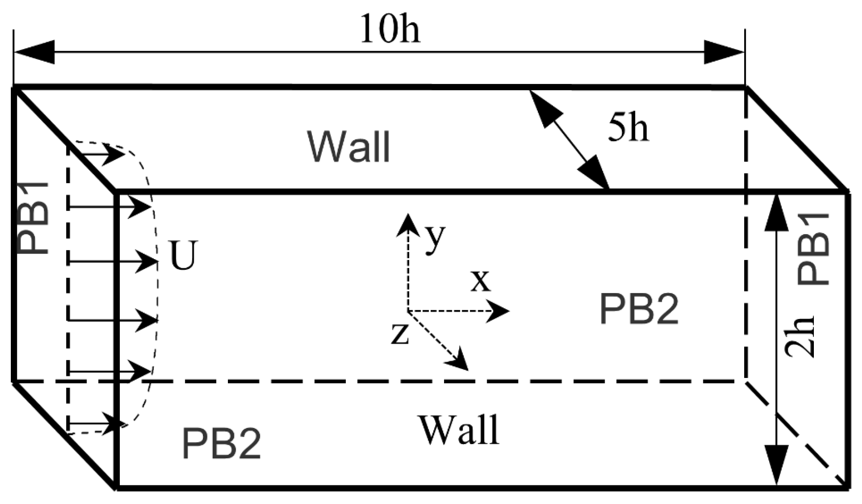
Figure 2.
Comparison of between the current work and the DNS data. The Dean curve represents the theoretical velocity of the Newtonian fluid. Virk is the fluid velocity with the maximum theoretical drag reduction.
Figure 2.
Comparison of between the current work and the DNS data. The Dean curve represents the theoretical velocity of the Newtonian fluid. Virk is the fluid velocity with the maximum theoretical drag reduction.

Figure 3.
Comparison of and between the current work and the DNS data. denotes the dimensionless turbulent kinetic energy and denotes the dimensionless wall-normal fluctuating velocity variance.
Figure 3.
Comparison of and between the current work and the DNS data. denotes the dimensionless turbulent kinetic energy and denotes the dimensionless wall-normal fluctuating velocity variance.
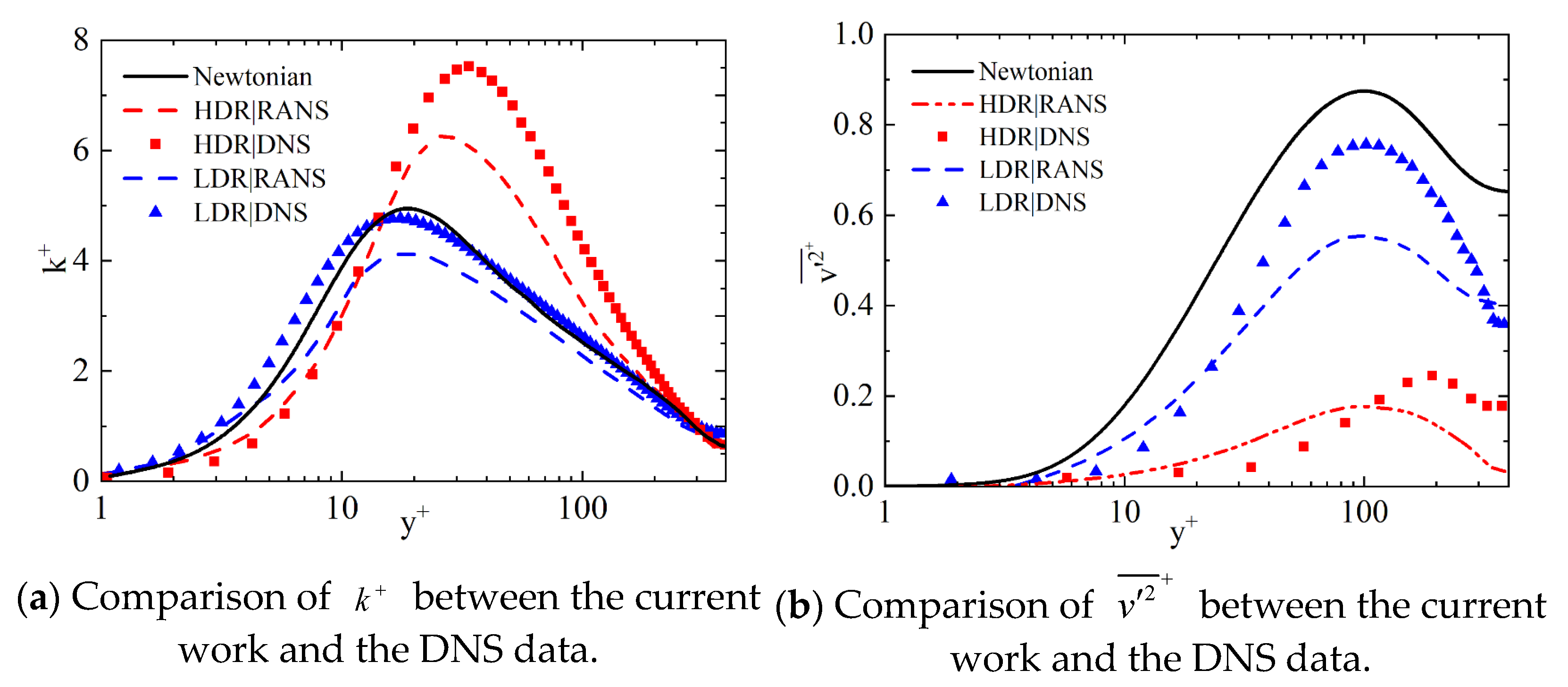
Figure 4.
Comparison of between the current work and the DNS. is the dimensionless turbulent dissipation rate.
Figure 4.
Comparison of between the current work and the DNS. is the dimensionless turbulent dissipation rate.

Figure 5.
Comparison of between the current work and the DNS data. is the components of the conformation tensor. denotes the maximum extensibility of the polymer molecule.
Figure 5.
Comparison of between the current work and the DNS data. is the components of the conformation tensor. denotes the maximum extensibility of the polymer molecule.
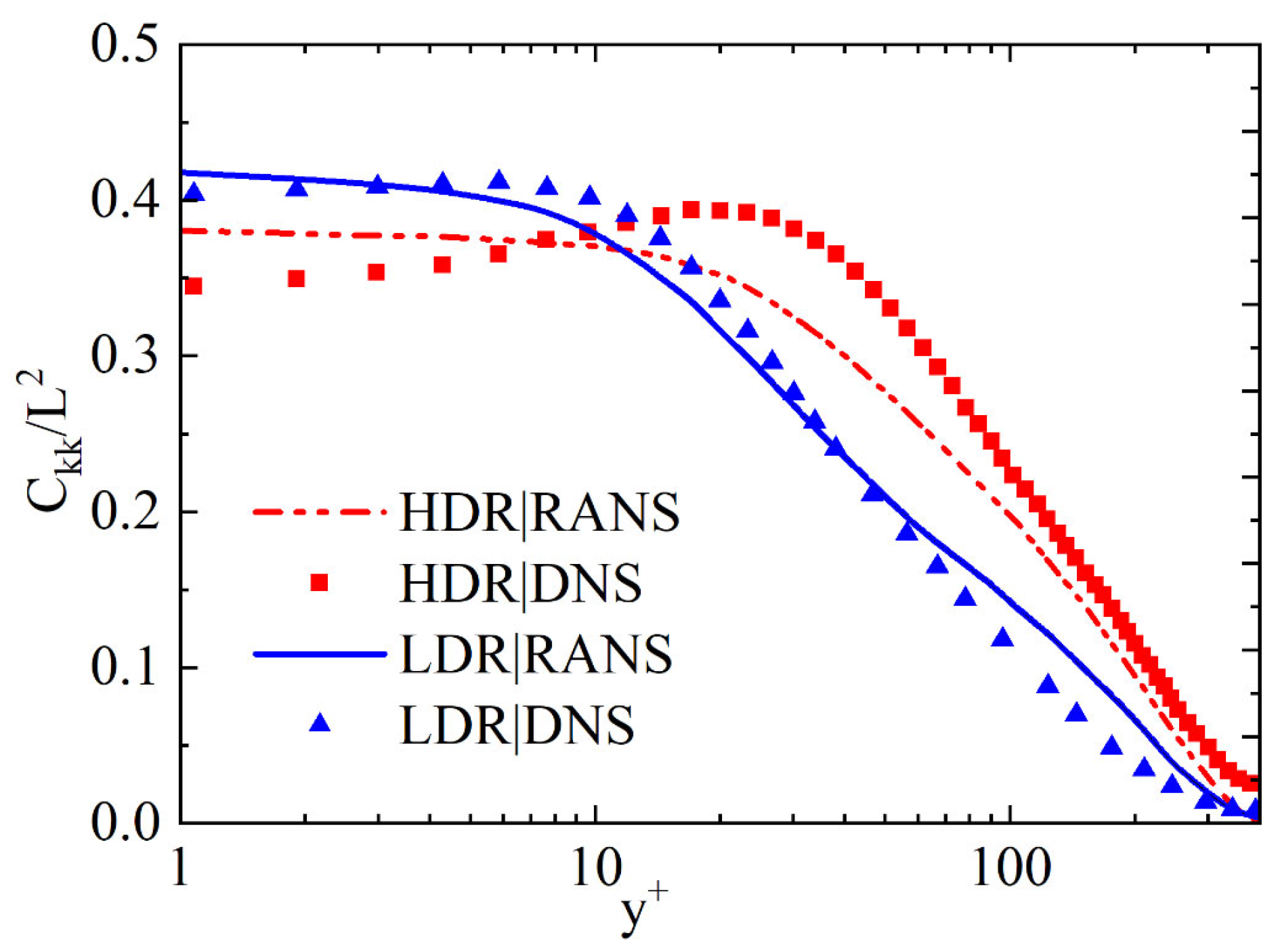
Figure 6.
Computational domain for the pipe flow. The left and right sides are the periodic boundary conditions.
Figure 6.
Computational domain for the pipe flow. The left and right sides are the periodic boundary conditions.
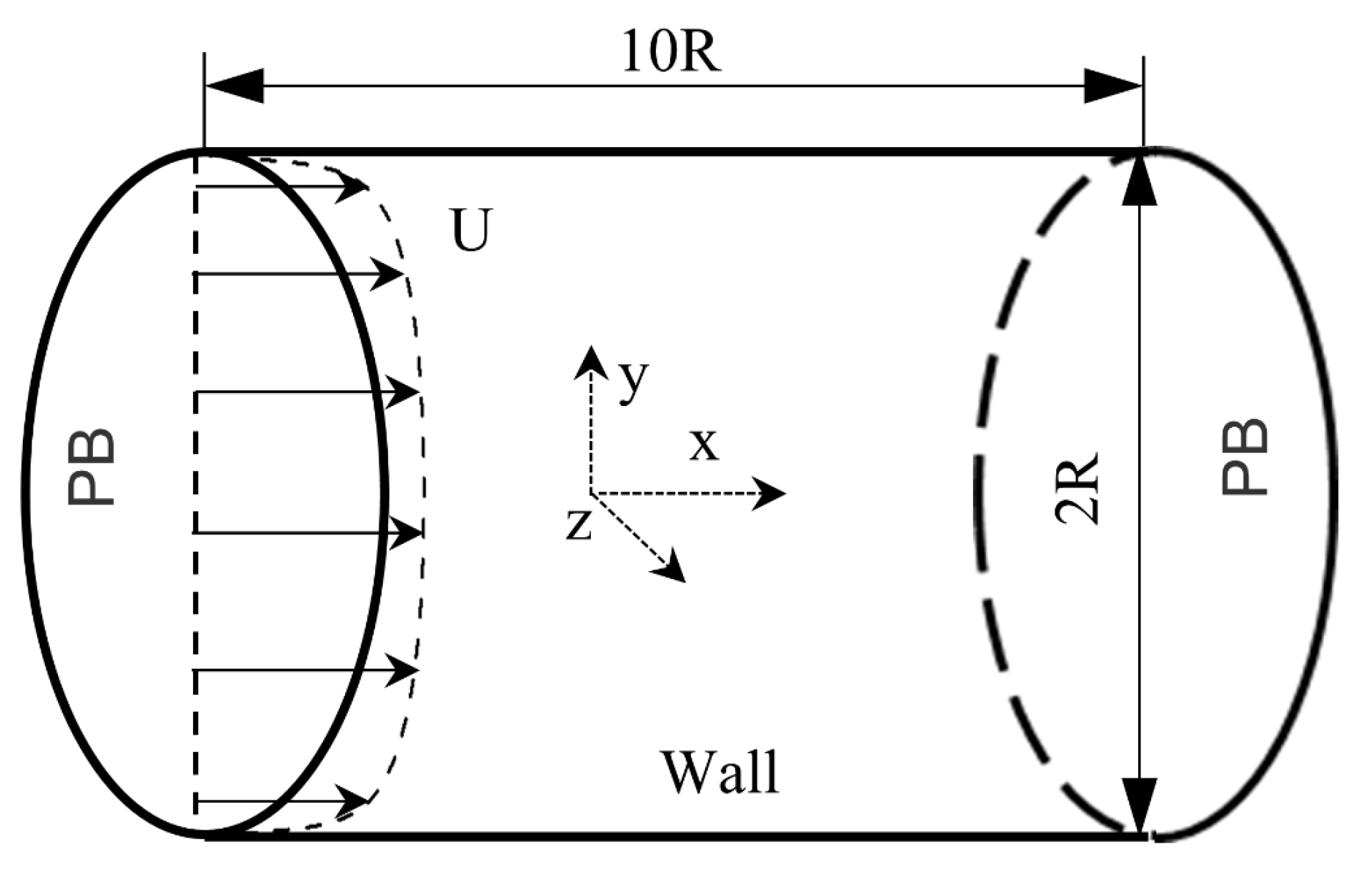
Figure 7.
Grid and grid independence verification results of pipeline flow.

Figure 8.
Drag reduction rate of different maximum extensibility of the polymer molecule (L).
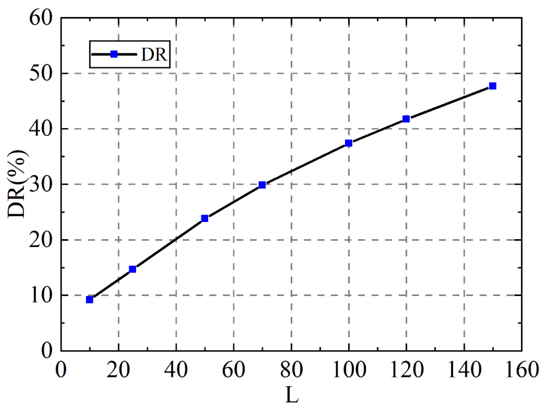
Figure 9.
Dimensionless average flow velocity () of different maximum extensibility of the polymer molecule (L).
Figure 9.
Dimensionless average flow velocity () of different maximum extensibility of the polymer molecule (L).

Figure 10.
Dimensionless turbulent kinetic energy () of different maximum extensibility of the polymer molecule (L).
Figure 10.
Dimensionless turbulent kinetic energy () of different maximum extensibility of the polymer molecule (L).
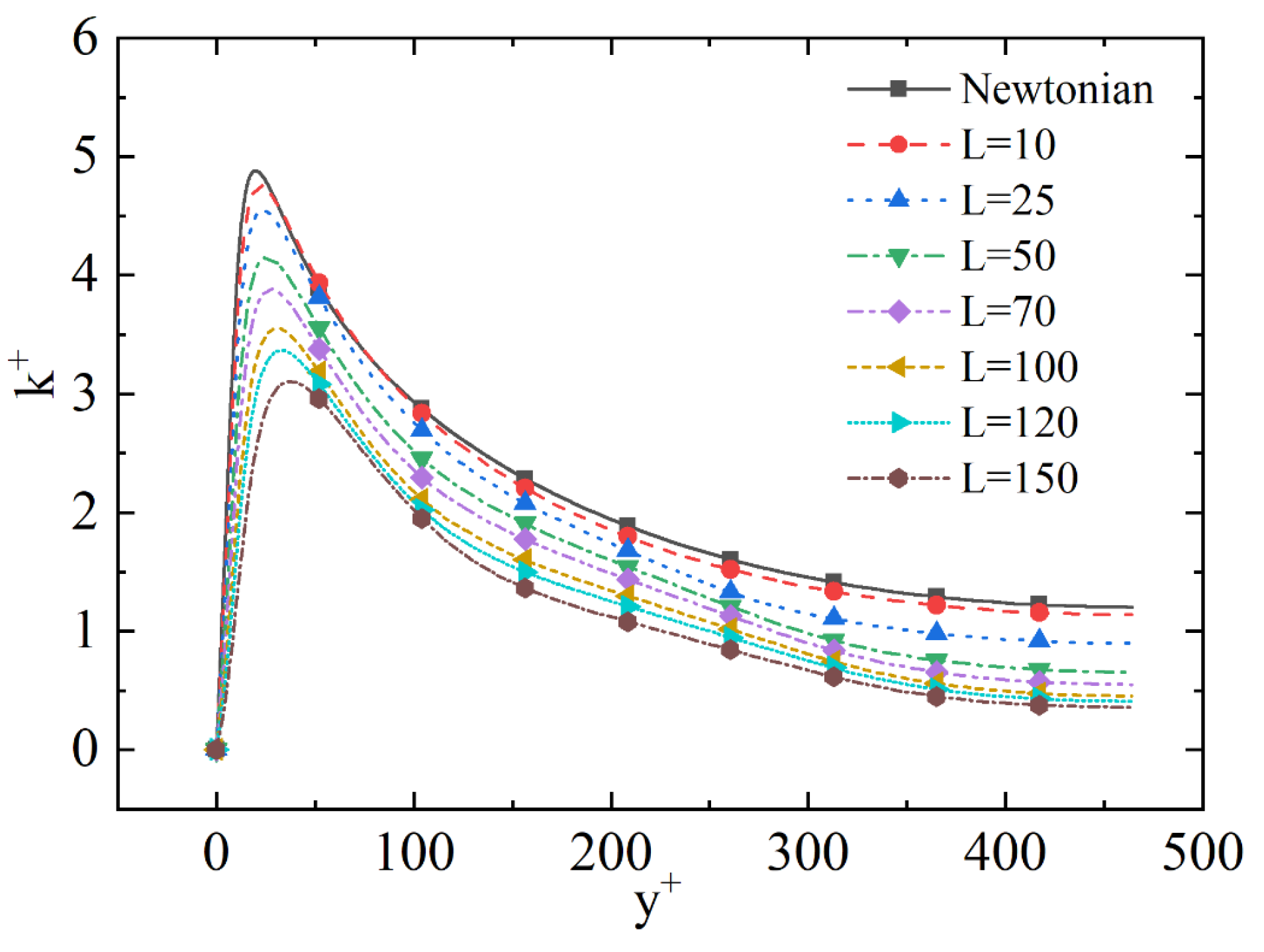
Figure 11.
Dimensionless variance of the wall−normal fluctuating velocity () of different maximum extensibility of the polymer molecule (L).
Figure 11.
Dimensionless variance of the wall−normal fluctuating velocity () of different maximum extensibility of the polymer molecule (L).
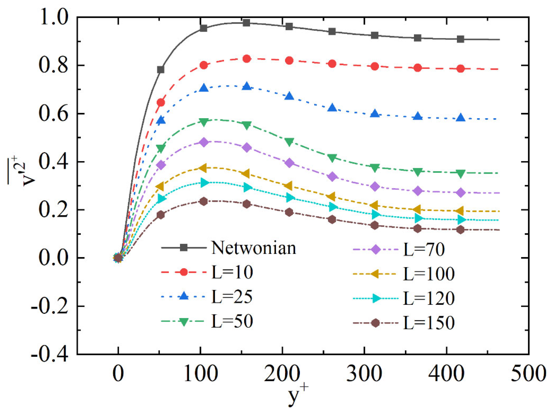
Figure 12.
Dimensionless turbulent dissipation rate (
of different maximum extensibility of the polymer molecule (L).
Figure 12.
Dimensionless turbulent dissipation rate (
of different maximum extensibility of the polymer molecule (L).

Figure 13.
Dimensionless component of the conformation tensor () of different maximum extensibility of the polymer molecule (L).
Figure 13.
Dimensionless component of the conformation tensor () of different maximum extensibility of the polymer molecule (L).
Figure 14.
Drag reduction rate of different Weissenberg numbers ().
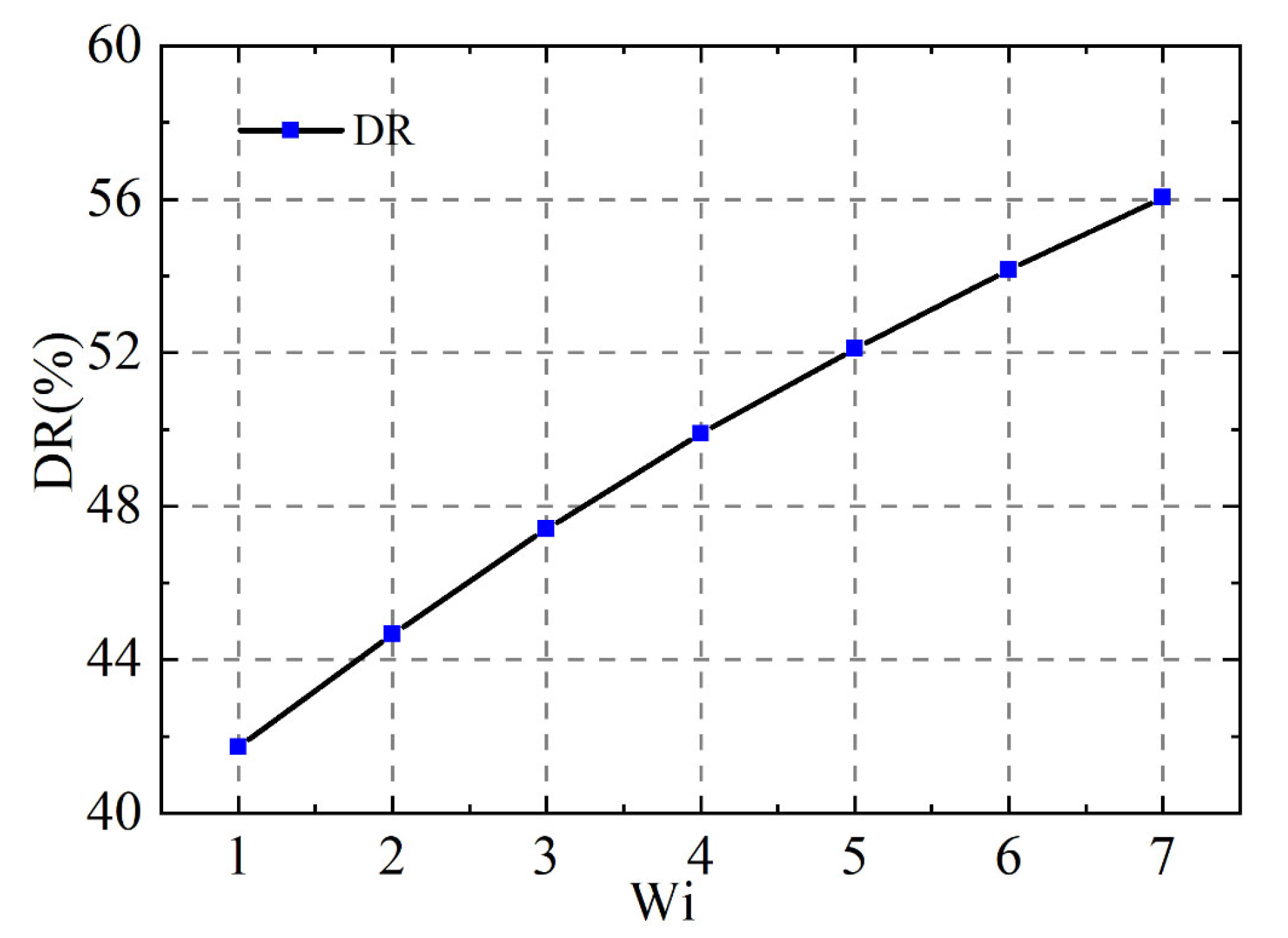
Figure 15.
Dimensionless average flow velocity () of different Weissenberg numbers ( ).
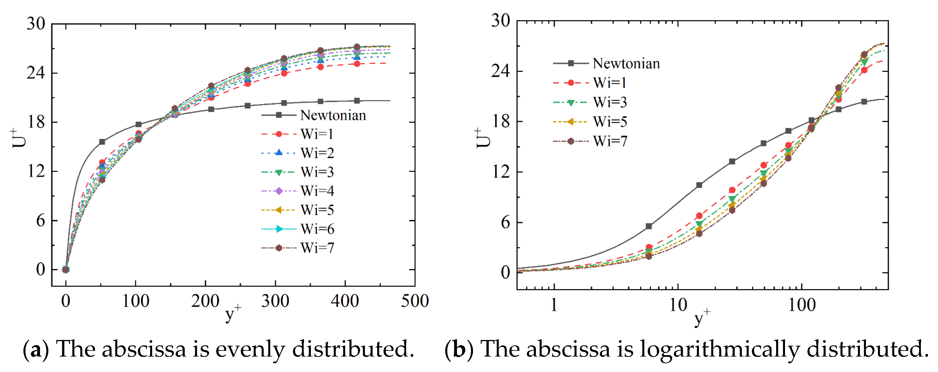
Figure 16.
Dimensionless turbulent kinetic energy () of different Weissenberg numbers ( ).

Figure 17.
Dimensionless turbulent dissipation rate () of different Weissenberg numbers ( ).
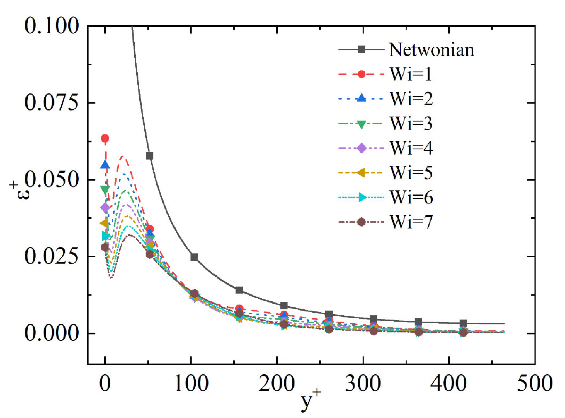
Figure 18.
Drag reduction rate of different solvent viscosity ratios ().
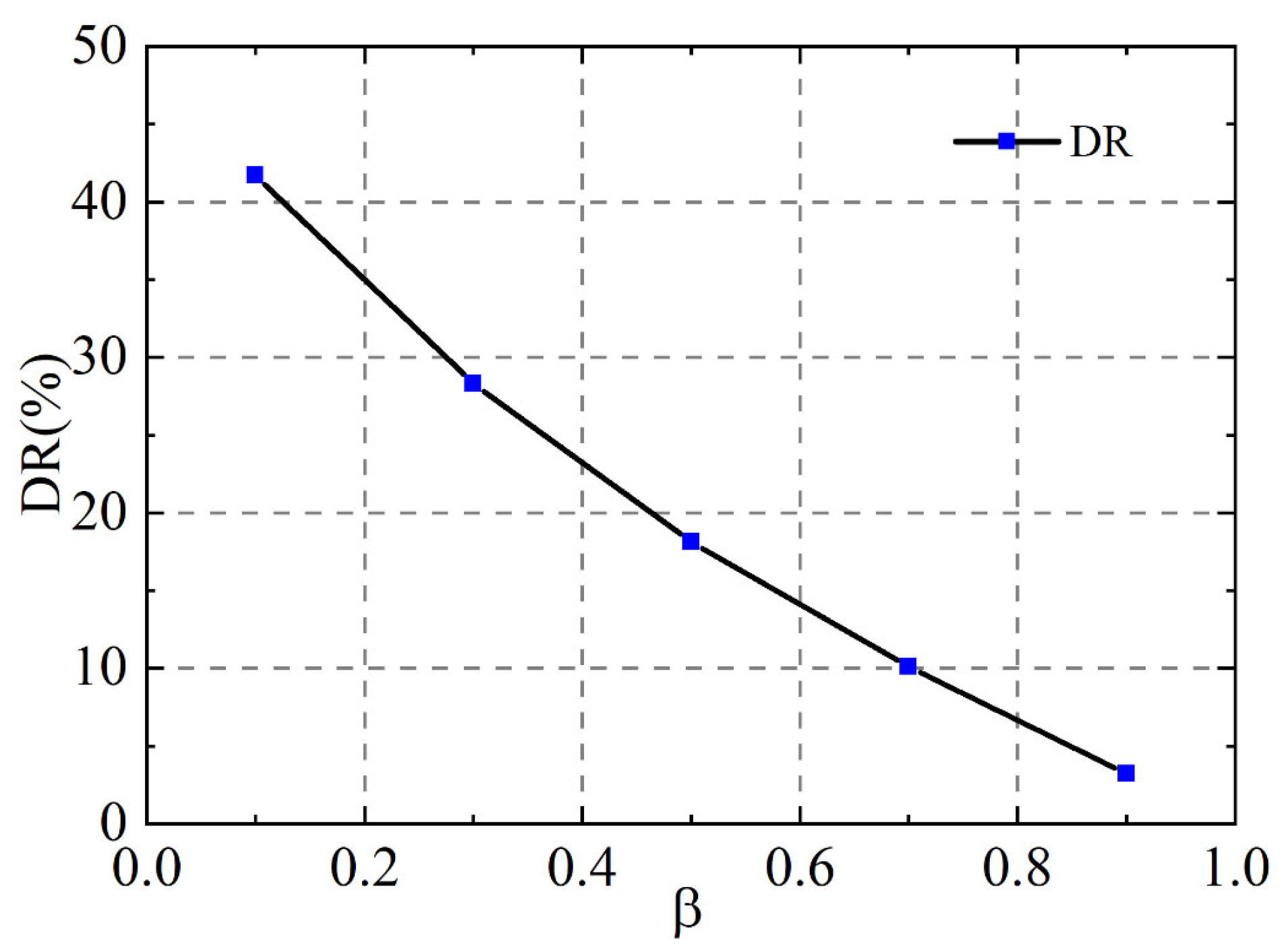
Figure 19.
Dimensionless average flow velocity () of different solvent viscosity ratios ( ).
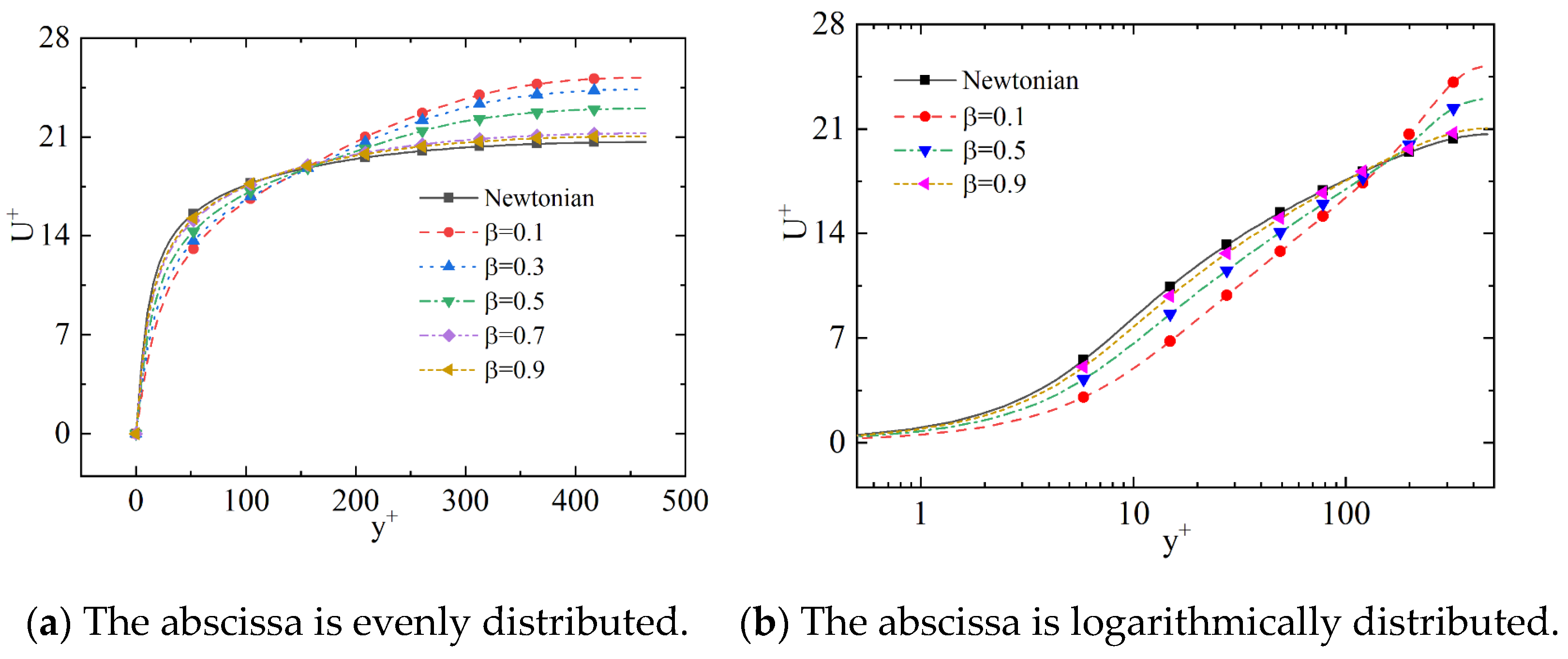
Figure 20.
Dimensionless turbulent kinetic energy () of different solvent viscosity ratios ( ).
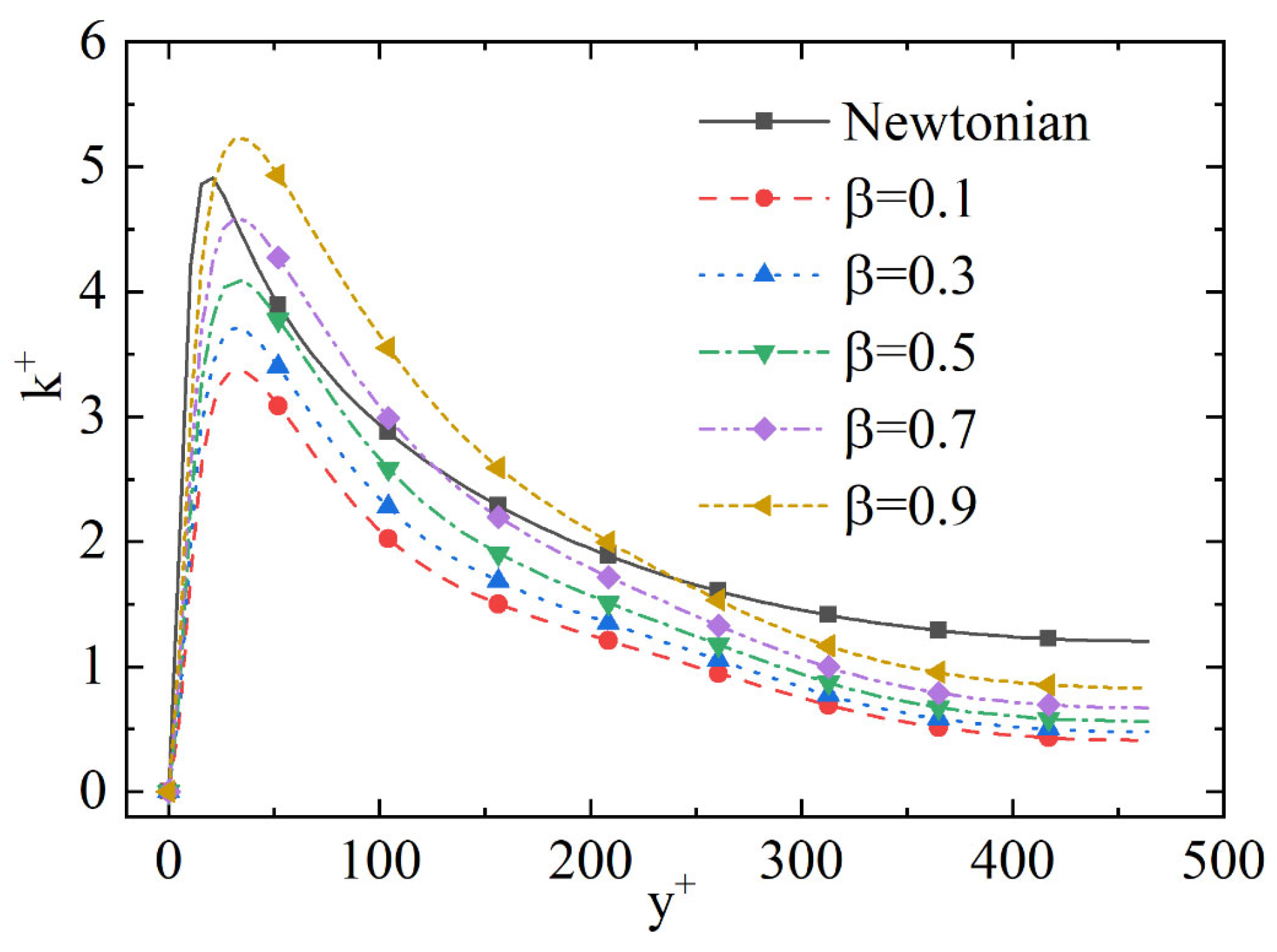
Figure 21.
Dimensionless turbulent dissipation rate () of different solvent viscosity ratios ( ).

Table 1.
Parameters of the two channel flow cases. LDR and HDR means a low and high DR rate, respectively. denotes the Reynold number. represents the Weissenberg number. represents the maximum extensibility of the polymer. represents the solvent viscosity ratio.
Table 1.
Parameters of the two channel flow cases. LDR and HDR means a low and high DR rate, respectively. denotes the Reynold number. represents the Weissenberg number. represents the maximum extensibility of the polymer. represents the solvent viscosity ratio.
| Case | DR (%) | ||||
|---|---|---|---|---|---|
| LDR | 395 | 25 | 900 | 0.9 | 18 |
| HDR | 395 | 100 | 14,400 | 0.9 | 63 |
Table 2.
Parameters for the pipe flow cases. , , and represent the Weissenberg number, maximum extensibility of the polymer molecule, and the solvent viscosity ratio, respectively.
Table 2.
Parameters for the pipe flow cases. , , and represent the Weissenberg number, maximum extensibility of the polymer molecule, and the solvent viscosity ratio, respectively.
| Case | |||
|---|---|---|---|
| A | 120 | 1 | 0.1 |
| B–G | 10, 25, 50, 70, 100, 150 | 1 | 0.1 |
| H–M | 120 | 2, 3, 4, 5, 6, 7 | 0.1 |
| N–Q | 120 | 1 | 0.3, 0.5, 0.7, 0.9 |
Disclaimer/Publisher’s Note: The statements, opinions and data contained in all publications are solely those of the individual author(s) and contributor(s) and not of MDPI and/or the editor(s). MDPI and/or the editor(s) disclaim responsibility for any injury to people or property resulting from any ideas, methods, instructions or products referred to in the content. |
© 2023 by the authors. Licensee MDPI, Basel, Switzerland. This article is an open access article distributed under the terms and conditions of the Creative Commons Attribution (CC BY) license (https://creativecommons.org/licenses/by/4.0/).
Share and Cite
MDPI and ACS Style
Li, Z.; Hu, H.; Du, P.; Xie, L.; Wen, J.; Chen, X. Reynolds-Averaged Simulation of Drag Reduction in Viscoelastic Pipe Flow with a Fixed Mass Flow Rate. J. Mar. Sci. Eng. 2023, 11, 685. https://doi.org/10.3390/jmse11040685
AMA Style
Li Z, Hu H, Du P, Xie L, Wen J, Chen X. Reynolds-Averaged Simulation of Drag Reduction in Viscoelastic Pipe Flow with a Fixed Mass Flow Rate. Journal of Marine Science and Engineering. 2023; 11(4):685. https://doi.org/10.3390/jmse11040685
Chicago/Turabian StyleLi, Zhuoyue, Haibao Hu, Peng Du, Luo Xie, Jun Wen, and Xiaopeng Chen. 2023. "Reynolds-Averaged Simulation of Drag Reduction in Viscoelastic Pipe Flow with a Fixed Mass Flow Rate" Journal of Marine Science and Engineering 11, no. 4: 685. https://doi.org/10.3390/jmse11040685
Note that from the first issue of 2016, this journal uses article numbers instead of page numbers. See further details here.