

Sea Floor Characterization by Multiples’ Amplitudes in Monochannel Surveys

National Institute of Oceanography and Applied Geophysics—OGS, 34010 Sgonico, Italy
*
Author to whom correspondence should be addressed.
J. Mar. Sci. Eng. 2023, 11(9), 1662; https://doi.org/10.3390/jmse11091662
Submission received: 13 July 2023
/
Revised: 22 August 2023
/
Accepted: 23 August 2023
/
Published: 24 August 2023
(This article belongs to the Topic Development of Monitoring, Analysis and Maintenance Technics of Infrastructures)
Abstract
:The lithological characterization of the seafloor is key information for offshore engineering, especially when it comes to pier and platform design. Undetected shallow gas pockets may cause the collapse of heavy platforms for hydrocarbon production. Unconsolidated sediments are not ideal for the basement of wind farms for electric power production. Drilling and coring can be used for local sampling, but continuous profiles or even areal coverage are far more preferable. High-resolution seismic profiles are successfully used when ports are not too busy, but otherwise, single-channel systems must be used. We show in this paper that even these simpler systems can be used to estimate parameters such as the acoustic impedance of shallow sediments directly beneath the seafloor. We exploit the amplitude decay of the multiple reflections between the seafloor and the surface, which does not depend on the source energy. If the offset between source and receiver is not too small, we can estimate the shallow P velocity and, via acoustic impedance, also the rock density.
1. Introduction
Offshore engineering requires extensive measurements of seabed properties when building pipelines, piers, or platforms, or even when laying communication cables. For example, undetected shallow gas pockets can cause the collapse of heavy platforms for hydrocarbon production. On the opposite side, muddy sediments are preferable for the deployment of communication cables, as they may sink there and be better protected from fishes and human activities. Lithological parameters such as elastic moduli and density are needed for planning foundations and excavations, especially for offshore wind farms. High-resolution seismic profiles are a viable solution for the marine environment, requiring simpler processing and a faster and cheaper acquisition than land profiles; also, multichannel surveys are now a mature technology. Advanced processing techniques such as full-waveform imaging can provide not only the above parameters, but also anisotropy (see [1,2,3], among others) and anelastic absorption [4,5,6]. However, this information relies on multichannel recording systems that are expensive and difficult to manage in busy areas such as harbors [7,8] or sensitive environments such as shallow lagoons or marine protected areas [9,10,11,12], or even in archeological applications [13,14,15,16]. In the latter cases, small boats with a short streamer are appropriate, using only one source and one receiver spaced a few meters apart [17,18,19]. In this paper, we show that even this parsimonious recording apparatus allows for the estimation of velocity and density of shallow sediments directly beneath the seafloor by exploiting the amplitude of multiple reflections. Ref. [20] showed that combining Chirp and Boomer data provides good estimates of the acoustic impedance of these sediments. Boomer sources emit an acoustic pulse from a plate floating at a depth of 10–30 cm from the sea surface. Their signal can be compared to that of airguns, but at higher frequencies and lower power. Chirp sources instead emit a longer signal, similar to the sweep of Vibroseis sources, so a cross-correlation between the source signal and the recorded signal is required to interpret and compare it to impulsive signals. The source and receiver are embedded in the same piezoelectric device, so their offset is zero, whereas it is typically between 3 and 10 m for Boomer systems. For further analysis on the processing of Chirp and Boomer data, we refer the reader to [21,22,23,24,25,26], among others.
2. Materials and Methods
The first step in characterizing the seafloor is to measure seawater depth and P velocity. These values can be obtained by inverting the travel times of direct arrivals and reflections at the seafloor or with a standard sonar and using seawater temperature [27]. The second step is to estimate the P velocity of shallow sediments, and possibly their thickness. Tomographic inversion of primary and multiple reflections can provide fair estimates for these parameters if the offset between source and receiver is not too small, e.g., 10 m [28,29]. The sediment P velocity is an important piece of information for offshore engineering, but we want to go a step further in this paper, i.e., obtain an indication of its density. To this goal, we will analyze the amplitude of the multiples to quantify the reflectivity of the seafloor, which is a function of the velocity and density contrasts between sediments and seawater. This information is also relevant for later processing steps, such as removing multiples to improve imaging of shallow sediments [30].
2.1. Amplitude of Multiple Reflections
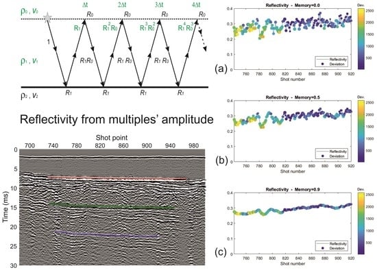
Seismic data contain information in signal amplitude (in its original waveform) or energy (in its envelope). In marine surveys, multiple reflections between the sea surface and the seafloor allow for the characterization of the shallowest formation directly beneath the seafloor. For Chirp data, the offset between source and receiver is zero, so we prefer to model the Earth only in 1D, or at most, in 1.5 D. We apply Occam’s razor principle to our estimation and avoid introducing parameters that cannot be constrained by the available data [31]. Figure 1 shows the reverberation of a unit pulse signal between the sea surface and the sea floor. For graphical convenience only, the ray paths are presented as slanted lines, whereas the intended propagation in the following mathematics is purely vertical. We have marked the measurable values in green and the values we estimate in black.
The two-way travel time for each bounce between the surface and the seafloor is t. At each reflection, the amplitude of the signal is multiplied by two factors: the air–water contact (R0) and the seafloor (R1). The accumulated amplitude variations are summarized in Table 1, assuming that there is no amplitude decay due to either anelastic absorption or geometrical spreading.
The air–water reflection coefficient R0 can be easily computed using the P velocity of air and sea water (343 and 1500 m/s, respectively) and their density (1.225 and 997 kg/m3, respectively; see also [23,27]), using the classical 1D relation for the interface between two media:
where ρi are the densities and vi are the P velocities of adjacent formations A and B. The obtained value 0.999438 for R0 is well approximated by 1, which stands for a total reflection. In practical experiments, however, the amount of energy injected downwards from the source into the seawater is not perfectly controlled because weather conditions and navigation instabilities can change at each shot point. Variations occur for the source depth, direction of the main lobe in the radiation pattern, and even waves at the sea surface. Therefore, a multiplier S must be added to the amplitude terms in Table 1, which is the same for each multiple reflection produced by the corresponding primary pulse. In principle, it can be different for each shot, but we found in our experience that this parameter is less critical than others as, for example, the offset between source and receiver [28,29]. The value S can be well approximated by the recorded amplitude of the direct arrival at each shot point.
R = (ρB vB − ρA vB)/(ρB vB + ρA vB)
Let us indicate by A1, A2, …, Aj the amplitude of the signals recorded at the sea surface at times ∆t, 2 ∆t, …, j ∆t. We can write the following linear equation system:
or, in a compact general form:
A1 = S R1
A2 = S R12 R0
A3 = S R13 R02
A4 = S R14 R03
Substituting (2) into (3), we obtain:
and rearranging, we obtain the product R0 R1:
A2 = A1 R1 R0
If we substitute (3) into (4), we obtain:
A3 = A2 R1 R0
Rearranging, we obtain again the product R0 R1:
We can proceed in the same way for any higher-order couple of multiples. Thus, the seafloor reflection coefficient can be obtained by the amplitude ratio of two consecutive multiples, for an elastic 1D Earth model:
as R0 is very close to 1. We remark that the unknown amplitude M of the source signal is irrelevant for the reflectivity calculation.
Strictly speaking, R0 approximates 1 only for conventional Chirp data, because the envelope operator applied to the original waveform converts the signal to a positive function. In this way, the polarity information is lost. For Boomer and original (non-enveloped) Chirp data, any reflection from the sea surface reverses the polarity of the signal, so that R0 actually approximates −1 and the relation (11) must be modified accordingly.
Merging Equations (8) and (10), we obtain:
Equation (12) shows that the amplitude ratio of two consecutive multiples is a constant. This property can be exploited in two ways. First, if large differences are found, the geometrical spreading compensation may need to be adjusted, e.g., by correcting for seawater velocity. Second, if the two ratios are comparable, their average could be taken to statistically consolidate this information.
Manipulating (1), we can express the acoustic impedance ρ2 v2 of the sea floor as a function of its reflectivity:
where ρ1 and v1 are density and P velocity of the sea water, while ρ2 and v2 are those ones of the seafloor sediments. Water parameters can be estimated independently, e.g., by measuring the temperature and salinity of seawater.
2.2. Spherical Divergence Correction
The above equations apply to a 1D propagation of plane waves incident perpendicularly on an interface. Chirp or Boomer experiments are better approximated by a point source emitting a signal, and seawater by a homogeneous isotropic elastic medium. Under these assumptions, the shape of the wavefront is a sphere that expands with time. Since the energy losses are negligible, the total energy of the wavefront is constant at all times. For simplicity, we choose the signal to be a spike with amplitude a(t). Due to the spherical symmetry of the propagation, this value is the same at every point of the wavefront at a given time. The energy E(t) at the travel times t1 and t2 must be the same, i.e., the surface integrals of the squared amplitude over the spherical wavefronts W1 and W2 are equal:
Simplifying (14) by 4π and taking the square root, we obtain:
r1 a(r1) = r2 a(r2)
If we set to 1 the amplitude a(r1) at the distance r1 = 1, we obtain:
a(r2) = 1/r2
We may move from the space to the time domain using the linear link between propagation time t and wavefront radius r for our simple case, obtaining:
where vsw is the P-wave velocity of the sea water. Equation (17) states that by multiplying the signal by vsw t, we compensate for the amplitude decay due to the geometrical spreading of energy over spherical wavefronts that expand in time. In this way, we reconcile the amplitude measurements in our 3D world with a simpler 1D Earth model.
a(t) = 1/(vsw t) = (vsw t)−1
The function (17) for the amplitude a(t) is valid for propagation in a homogeneous elastic medium. This assumption is quite well satisfied by seawater over a short distance. When considering deeper reflections, the seismic waves propagate through rock layers that absorb much of their energy, and thus strongly affect the signal amplitude. Compensation for this absorption is also possible for single-channel data [32,33]; however, since this propagation effect is negligible in our case [34,35,36], we omit this further correction.
To account for both geometrical spreading and reflection coefficients R0 and R1, Equation (6) must be multiplied by (17). In compact form, they can be expressed as follows:
We can compensate part of the geometrical spreading by multiplying the multiples’ amplitudes Aj in (17) by their traveltime j ∆t, obtaining:
We note that the only significant difference between Equations (6) and (19) is the additional factor 1/vsw. This relation allows us to check the accuracy of the seawater velocity vsw and possibly correct it at each shot point based on the misfit between the experimental amplitude values and those modeled by (19), where the prime index represents a multiplication by the corresponding traveltime.
2.3. Reflectivity Robustness by Physical Constraints
The measured amplitudes are normally affected by errors, due to picking errors or interfering events, especially for late or weak multiples. To obtain a robust reflectivity estimation, we may exploit the physical constraint implied by (12), which may be rewritten as:
We define an object function O(Aj) as the sum of their squared differences between the measured amplitudes and the trial amplitude values Aj′:
where v indicates a trial velocity. We limit the j index to 3, so considering the amplitudes of a primary and its first and second multiple. The actual value of the seawater velocity is implicit in the measured amplitude and need not to be measured directly in this approach: it is highlighted in (21) to remark that its value may be tuned shot by shot.
The Aj terms in (21) depend on S and R1 only, if we set R0 to be 1 in (6). Therefore, we have three unknowns S, R1 and vsw, which requires at least three measurements to be estimated: the sea floor primary and two multiple reflections. Higher-order multiples might be added to constrain the solution further, but they are mostly weak and noisy, so we ignore this option.
To validate the use of this object function, we built a simple 1D model with the three key parameters: sea water velocity vsw = 1500 m/s, reflectivity R1 = 0.4, and source amplitude S = 1. The corresponding “true” amplitudes Aj′, given by (19), were perturbed by random errors uniformly distributed in a range of 20%, allowing for noise and picking errors, to simulate the values which we can obtain experimentally.
Figure 2 shows the estimates obtained by 200 perturbations (and similar results are obtained by other perturbation numbers). The perturbations are applied as random percentage errors, up to a maximum absolute value of 20%. The larger red dot is the true solution, while the large black dot is the average of all estimates. In Figure 2a, which uses the simple object function in (21), the average and true solution are very close, despite the significant dispersion of the other dots. Indeed, experimental scientists always use redundancy of measurements to increase the accuracy of their estimates. However, this is hardly possible for monochannel data, since each shot is a single measurement that is not repeated at the same location. For Boomer profiles, we could use a short streamer with a few receivers spaced the same distance as the shot interval. This way, we could obtain at least a couple of traces at each mid-point with source and receiver positions reversed, which could be averaged to increase the signal/noise ratio. This is not possible with Chirp systems, because the source and receiver coincide. However, we obtain some redundancy in other ways, by taking advantage of the very high spatial sampling (as shooting intervals of 30 cm are common) and the normally smooth lateral variations of seawater and shallow sediments. We can mix the estimate E = (v, R1, S) = E(x) at the current position x with that one at the preceding one:
where λ is a user-defined parameter ranging from zero to one. The lower λ is, the weaker the memory of past values is. When fluctuations are small, the memory factor is not relevant, whereas when fluctuations are rapid, it is substantial in our estimates. For example, a λ value of 0.5 implies averaging over two consecutive values, i.e., smoothing by a short moving average. As λ approaches 0, this smoothing effect disappears, but so does its stabilization. Values above 0.5 can lead to undesirable artifacts, as older values would prevail over current measurements.
Em(x, λ) = E(x) (1 − λ) + E(x − ∆x) λ
Figure 2b shows that the solutions’ dispersion is much smaller when the memory parameter λ is set to 0.5. The average percentage error of reflectivity is reduced from 11.2% to 5.7% in this example.
The colors of the dots in Figure 2 represent a property of the input data that we defined in view of the ideal case in (20): it applies to noise-free data. Noise is always present in experimental data, so we expect this relationship to be violated in most cases. To quantify this deviation from the theoretical values, we defined a deviation function Dev as follows:
When the experimental values satisfy Equation (20), the deviation is zero; when is much larger or much smaller than , it approximates one. The colors in Figure 2 present the deviation of the input data used to produce the estimation of that dot. Those ones with the largest deviation (yellow color) are noisier, and are more abundant in the dots that are distant from the true solution (the big red dot).
We may expect that the memory contribution of noisy data might damage the result, instead of improving it. For this reason, we modified the Formula (22) by introduction a contribution of the deviation Dev:
Emd(x, λ) = E(x) [1 − λ (1 − Dev)] + E(x − ∆x) λ Dev
When no memory factor is applied (Figure 2c), the improvement is marginal for the velocity and even worse for the reflectivity. However, when the memory is set to 0.5 and the deviation constraint is applied, we obtain the best result for the velocity and the second best for the reflectivity.
3. Results
3.1. Application to a Synthetic Survey
In 2D marine surveys, each shot is at a different point along a profile, so we cannot improve the signal noise by averaging, but can at most rely on the usual smoothness of geologic variations. To study a more realistic case, we simulated a profile of 200 shots in a 1D Earth model consisting only of the water layer overlying some sediments (Figure 3).
Water velocity decreases linearly from 1520 to 1480 m/s, while sediment velocity decreases from 2000 to 1600 m/s. Conversely, the water density is constant and set to 1, while the sediment density varies between 1.7 and 1.6 g/cc. Thus, the lateral changes in seafloor reflectivity depend on both the variations in seawater velocity and sediment density in this example. Water depth and sediment thickness also vary laterally in a smooth way. Water density is assumed to be constant, while sediment density decreases from 1.7 to 1.6 g/cc. As for the example in Figure 2, we calculated the correct amplitudes for primary and multiples using the actual model, assuming vertical propagation in a 1D model. Then, we randomly perturbed their values, with a maximum percentage of 20%. Finally, we inverted these noisy values using a memory factor of 0.5 weighted by the deviation function (23).
Figure 4 shows two views of the three-dimensional space of solutions whose axes are seawater velocity, seafloor reflectivity, and signal amplitude at the source. The red dots indicate the true solution, while the other dots represent the estimates, colored according to their deviation. The points’ dispersion is larger in the dimension of velocity than in the others. This fact becomes clearer when plotting these estimates on a graph: the reflectivity varies considerably (Figure 5a), but follows fairly closely the trend of the true model (red line). The estimated velocity varies much more (Figure 5b) and does not fit the linear trend of the true model (red line). Even the estimated average (cyan dotted line) does not match the average of the true model (green dotted line). Despite this disappointing result, the estimated acoustic impedance (Figure 5c) is acceptable: although it still oscillates, its trend fits the true curve quite well (red line), and the fit becomes good when the estimated values are smoothed by a moving-average filter with a window of 15 elements. The estimation of the density (Figure 5d) is only possible if we know the velocity of the seafloor sediments, which cannot be estimated by the method presented here, which is based only on the amplitude of the signals. However, it can be obtained by also inverting their travel times [28,29].
Assuming that the velocity of the sediments is known, we can also calculate the density of the seafloor sediments (Figure 5d). The estimated density is again wavy (blue line), but can reflect the correct trend (red line), and if we apply the smoothing filter mentioned above, we obtain a satisfactory result (green line).
In this example, we have used extreme values for seawater velocity that cover virtually the entire range normally encountered in marine surveys. In the real world, lateral variations are much more uniform and could, in principle, be measured independently. Therefore, we performed another inversion test where we assigned the correct water velocity and inverted for the other two parameters, i.e., seafloor reflectivity and source amplitude. Figure 6 shows that there are no major differences: only in Figure 2b do the true and “modeled” velocities overlap, since we forced them coincide. From this, we can conclude that the wavy estimates of the other parameters are mainly due to noise in the signal amplitudes, rather than crosstalk between errors in the velocity estimates. Consequently, we expect that improving the signal-to-noise ratio through proper data acquisition and preprocessing is the key to reliable estimates of the other parameters discussed here.
3.2. Application to a Real Marine Survey
We tested the inversion of amplitudes for a Boomer survey acquired off Asinara Island (Sardinia, Italy). The main recording parameters are summarized in Table 2. Figure 7 shows the recording geometry, with towed source and receiver divided by a gap of about 1 m, and a distance from the GPS positioning system of about 3 m.
Figure 8 shows parts of the recording system, i.e., the energy source (top) and the Boomer plate (bottom).
The data were acquired by OGS (Italian National Institute of Oceanography and Experimental Geophysics) in the framework of a survey committed by the Asinara Island National Park [37]. One of the objectives was to monitor the occurrence and distribution of Posidonia Oceanica, an endemic seagrass of the Mediterranean Sea that provides a good habitat for fish. In the area studied, the seafloor consists of coarse-to-fine sediments, including marine and eolian sandstones. There are also some paleo-fluvial valleys with fluvial conglomerates and gravel sands [37,38].
Figure 9 displays the seismic section obtained after geometrical spreading compensation using the simple function (17) and a seawater velocity of 1500 m/s. This is a default value that we chose because no direct or indirect measurements were made during the survey. The picked seafloor (red line) is slightly inclined, with travel times decreasing from 6 to 7 ms. The shallower event at about 2 ms is the direct arrival from the source to the receiver. The first multiple (green line) is a reverberation between the sea surface and the sea floor, as is the second multiple (blue line). The small unevenness of the seafloor near the 870 shot point facilitates the detection of the multiples from other primaries or multiples, as it is clearly visible in the picked events. Another positive control for the reliability of the picking is the polarity reversal that occurs in both multiples.
Since we need at least two multiples for our inversion, we limited our analysis to the shot points from 742 to 920 because the signals outside this range were overwhelmed by noise, diffractions, and other interfering events. Figure 10 shows the estimates obtained with different memory coefficients: from 0, i.e., no memory, to an intermediate value of 0.5, and to 0.9, corresponding to a long smoothing window. Regardless of which memory factor is used, the trend remains unchanged, i.e., it increases slightly from left to right. The colors of the dots depict the deviation of the experimental data from the optimal fit estimated in each shot using definition (23). The fit is very good (bluish values) in the center and right, becoming worse on the left. This slight change could be due to the presence of more diffractions and shallow reflections between the shot points 740 and 800 (Figure 9).
Figure 11 shows the reflectivity obtained by keeping fixed the memory coefficient at 0.9 but assuming different velocities for the sediments on the seafloor, i.e., 1800, 2000, and 2200 m/s. The reflectivity does not change, and so does the associated acoustic impedance. For their product to remain constant, an increase in velocity leads to a decrease in density. Thus, we need an accurate, independent estimate of sediment velocity to even approximate density.
4. Discussion and Conclusions
We have presented a new method for estimating the seafloor reflectivity through single-channel systems by exploiting the amplitude of the multiples. The method works quite well with synthetic data, especially when the signal-to-noise ratio is favorable. In this case, the reliability of the estimation is satisfactory. With real data, control over the actual signal-to-noise ratio is difficult to assess. We can only compare our estimates of P velocity and density with the typical values of the expected rocks in the area or, if available, with core measurements for calibration. In this way, we can detect and localize lateral variations in lithology that provide a semi-quantitative characterization of shallow marine sediments.
Although the problem is mathematically simple, experimental errors in the data can affect the stability of the estimate. For this reason, we defined a new algorithm that stabilizes the results by imposing physical and geological constraints.
The reflectivity of the seafloor directly provides the acoustic impedance of the shallow sediments, and thus also contributes to a possible estimate of their density. As a byproduct of the multiples’ picking, we can also invert their travel times and estimate their P velocity. We note that the latter estimates may be subject to considerable uncertainty, depending on data quality and the offset between source and receiver. If such a velocity is not available or not reliable, we still obtain a fair estimate of the acoustic impedance.
Reflectivity and impedance can characterize the seafloor for offshore engineering applications and potentially reveal lateral variations in seafloor lithology. For example, shallow gas pockets can be detected by lower P velocity and density, and by an increase in reflectivity. The main advantage of high-resolution profiling is its low cost and potential significant coverage, even in busy areas such as ports or in sensitive environments such as lagoons.
Author Contributions
Conceptualization, A.V. and L.B.; methodology, A.V. and L.B.; software, A.V.; validation, A.V. and L.B.; formal analysis, A.V. and L.B.; investigation, A.V. and L.B.; resources, L.B.; data curation, L.B.; writing—original draft preparation, A.V.; writing—review and editing, A.V. and L.B.; visualization, A.V. and L.B.; supervision, L.B.; project administration, L.B.; funding acquisition, L.B. All authors have read and agreed to the published version of the manuscript.
Funding
This research received no external funding.
Institutional Review Board Statement
Not applicable.
Informed Consent Statement
Not applicable.
Data Availability Statement
The experimental data may be provided upon request to Luca Baradello ([email protected]), while the synthetic data and the computer codes may be provided upon request to Aldo Vesnaver ([email protected]). The codes may not be used for commercial purposes.
Acknowledgments
The marine seismic survey was acquired by OGS, committed by the Asinara Island National Park to conduct a series of geophysical surveys both offshore and onshore in the area of the Asinara Island.
Conflicts of Interest
The authors declare no conflict of interest.
References
- Alkhalifah, T.A. Full Waveform Inversion in an Anisotropic World; Education Tour Series; EAGE: Houten, The Netherlands, 2014; 197p, ISBN 9789462822023. [Google Scholar]
- Owusu, J.C.; Podgornova, O.; Charara, M.; Leaney, S.; Campbell, A.; Ali, S.; Borodin, I.; Nutt, L.; Menkiti, H. Anisotropic elastic full-waveform inversion of walkaway vertical seismic profiling data from the Arabian Gulf. Geophys. Prospect. 2016, 64, 38–53. [Google Scholar] [CrossRef]
- Huang, X.; Solberg Eikrem, K.; Jakobsen, M.; Nævdal, G. Bayesian full-waveform inversion in anisotropic elastic media using the iterated extended Kalman filter. Geophysics 2020, 85, C125–C139. [Google Scholar] [CrossRef]
- Askan, A.; Akcelik, V.; Bielak, J.; Ghattas, O. Full waveform inversion for seismic velocity and anelastic losses in heterogeneous structures. Bull. Seismol. Soc. Am. 2007, 97, 1990–2008. [Google Scholar] [CrossRef]
- Komatitsch, D.; Xie, Z.; Bozdağ, E.; Sales de Andrade, E.; Peter, D.; Liu, Q.; Tromp, J. Anelastic sensitivity kernels with parsimonious storage for adjoint tomography and full waveform inversion. Geophys. J. Int. 2016, 206, 1467–1478. [Google Scholar] [CrossRef]
- Vesnaver, A.; Lin, R. Broadband Q-factor tomography for reservoir monitoring. J. Appl. Geophys. 2019, 165, 1–15. [Google Scholar] [CrossRef]
- Maurenbrecher, P.M.; Wever, T. H-Sense’: Harbour sediment mapping using Chirp reflection surveys in Norway and Sweden. Expanded Abstract. In Proceedings of the 4th EEGS Meeting, Barcelona, Spain, 14–17 September 1998. cp-43-00065. [Google Scholar] [CrossRef]
- Barsottelli-Botelho, M.A.; Mesquita, L. Using GPR and high frequency seismic to locate under water buried pipes. Extended Abstracts. In Proceedings of the Near Surface Geoscience Conference, Turin, Italy, 6–10 September 2015. We21P104. [Google Scholar] [CrossRef]
- Richardson, W.J.; Greene, C.R.; Malme, C.I.; Thomson, D.H. Marine Mammals and Noise; Academic Press: San Diego, CA, USA, 1998; ISBN 9780080573038. [Google Scholar]
- Gordon, J.; Gillespie, D.; Potter, J.; Frantzis, A.; Simmonds, M.P.; Swift, R.; Thompson, D. A review of the effects of seismic surveys on marine mammals. Mar. Technol. Soc. J. 2003, 37, 16–34. [Google Scholar] [CrossRef]
- Baradello, L.; Carcione, J.M. Optimal seismic-data acquisition in very shallow waters: Surveys in the Venice lagoon. Geophysics 2008, 73, Q59–Q63. [Google Scholar] [CrossRef]
- Tosi, L.; Rizzetto, F.; Zecchin, M.; Brancolini, G.; Baradello, L. Morphostratigraphic framework of the Venice Lagoon (Italy) by very shallow water VHRS surveys: Evidence of radical changes triggered by human-induced river diversions. Geophys. Res. Lett. 2009, 36, 1–5. [Google Scholar] [CrossRef]
- Quinn, R.; Bull, J.M.; Dix, J.K. Imaging wooden artefacts using Chirp sources. Archaeol. Prospect. 1997, 4, 25–35. [Google Scholar] [CrossRef]
- Quinn, R.; Bull, J.M.; Dix, J.K. Optimal processing of marine high resolution seismic reflection (Chirp) data. Mar. Geophys. Res. 1998, 20, 13–20. [Google Scholar] [CrossRef]
- Plets, R.M.K.; Dix, J.K.; Best, A.I. Mapping of the buried Yarmouth roads wreck, isle of Wight, UK, using a Chirp sub-bottom profiler. Int. J. Naut. Archaeol. 2008, 37, 360–373. [Google Scholar] [CrossRef]
- Kim, Y.J.; Koo, N.H.; Cheong, S.H.; Kim, J.K.; Seo, K.S.; Hwang, K.D.; Kim, C.S.; Lee, H.Y.; Kim, W.S. A case study of 3D Chirp sub-bottom profiles survey at ancient wooden shipwreck site in Korea. Expanded Abstracts. In Proceedings of the Near Surface Geoscience Conference, Barcelona, Spain, 4–8 September 2016; pp. 1–5. [Google Scholar] [CrossRef]
- Gutowski, M.; Bull, J.; Henstock, T.; Dix, J.K.; Hogarth, P.; Leighton, T.; White, P. Chirp sub-bottom profiler source signature design and field testing. Mar. Geophys. Res. 2002, 23, 481–492. [Google Scholar] [CrossRef]
- Müller, C.; Milkereit, B.; Bohlen, T.; Theilen, F. Towards high-resolution 3D marine seismic surveying using Boomer sources. Geophys. Prospect. 2002, 50, 517–526. [Google Scholar] [CrossRef]
- Müller, C.; Woelz, S.; Ersoy, Y.; Boyce, J.; Jokisch, T.; Wendt, G.; Rabbel, W. Ultra-high-resolution 2D-3D seismic investigation of the Liman Tepe/Karantina Island archeological site (Urla/Turkey). J. Appl. Geophys. 2009, 68, 124–134. [Google Scholar] [CrossRef]
- Vardy, M.E. Deriving shallow-water sediment properties using post-stack acoustic impedance inversion. Near Surf. Geophys. 2015, 13, 143–154. [Google Scholar] [CrossRef]
- Schock, S.G.; LeBlanc, L.R.; Mayer, L.A. Chirp sub-bottom profiler for quantitative sediments analysis. Geophysics 1989, 54, 445–450. [Google Scholar] [CrossRef]
- Baradello, L. An improved processing sequence for uncorrelated Chirp sonar data. Mar. Geophys. Res. 2014, 35, 337–344. [Google Scholar] [CrossRef]
- Vardy, M.E. Remote characterization of shallow marine sediments—Current status and future questions. Extended Abstracts. In Proceedings of the Near Surface Geoscience Conference, Barcelona, Spain, 4–8 September 2016. MoASM05. [Google Scholar] [CrossRef]
- Faggetter, M.; Vardy, M.; Dix, J.; Bull, J.; Henstock, T. Time-lapse imaging of the shallow subsurface at decimetre scale resolution. Extended Abstracts. In Proceedings of the EAGE Annual Meeting, London, UK, 3–6 June 2019. WS02_11. [Google Scholar] [CrossRef]
- Boldreel, L.O.; Grøn, O.; Cvikel, D. Synthetic 3D Recording of a shipwreck embedded in seafloor sediments: Distinguishing internal details. Heritage 2021, 4, 541–553. [Google Scholar] [CrossRef]
- Kim, S.B.; Park, H.L. Optimizing source wavelets extracted from the Chirp sub-bottom profiler using an adaptive filter with machine learning. J. Mar. Sci. Eng. 2022, 10, 449. [Google Scholar] [CrossRef]
- Mackenzie, K.V. Nine-term equation for sound speed in the oceans. J. Acoust. Soc. Am. 1981, 70, 807–812. [Google Scholar] [CrossRef]
- Vesnaver, A.; Baradello, L. Shallow velocity estimation by multiples for monochannel Boomer surveys. Appl. Sci. 2022, 12, 3046. [Google Scholar] [CrossRef]
- Vesnaver, A.; Baradello, L. Tomographic joint inversion of direct arrivals, primaries and multiples for monochannel marine surveys. Geosciences 2022, 12, 219. [Google Scholar] [CrossRef]
- Schwardt, M.; Wilken, D.; Rabbel, W. Attenuation of seismic multiples in very shallow water: An application in archaeological prospection using data driven approaches. Remote Sens. 2021, 13, 1871. [Google Scholar] [CrossRef]
- Constable, S.C.; Parker, R.L.; Constable, C.G. Occam’s inversion: A practical algorithm for generating smooth models from electromagnetic sounding data. Geophysics 1987, 52, 289–300. [Google Scholar] [CrossRef]
- Claerbout, J. Imaging the Earth’s Interior; Blackwell: Oxford, UK, 1985; pp. 233–234. [Google Scholar]
- Denich, E.; Vesnaver, A.; Baradello, L. Amplitude recovery and deconvolution of Chirp and Boomer data for marine geology and offshore engineering. Energies 2021, 14, 5704. [Google Scholar] [CrossRef]
- Francois, R.E.; Garrison, G.R. Sound absorption based on ocean measurements: Part I:Pure water and magnesium sulfate contributions. J. Acoust. Soc. Am. 1982, 72, 896–907. [Google Scholar] [CrossRef]
- Francois, R.E.; Garrison, G.R. Sound absorption based on ocean measurements: Part II:Boric acid contribution and equation for total absorption. J. Acoust. Soc. Am. 1982, 72, 1879–1890. [Google Scholar] [CrossRef]
- Ainslie, M.A.; McColm, J.G. A simplified formula for viscous and chemical absorption in sea water. J. Acoust. Soc. Am. 1998, 103, 1671–1672. [Google Scholar] [CrossRef]
- Romeo, R.; Baradello, L.; Blanos, R.; Congiatu, P.P.; Cotterle, D.; Ciriaco, S.; Donda, F.; Deponte, M.; Gazale, V.; Gordini, E.; et al. Shallow geophysics of the Asinara Island Marine Reserve Area (NW Sardinia, Italy). J. Maps 2019, 15, 759–772. [Google Scholar] [CrossRef]
- Andreucci, S.; Pascucci, V.; Clemmensen, L. Upper Pleistocene coastal deposits of West Sardinia: A record of sea-level and climate change. GeoActa 2006, 5, 79–96. [Google Scholar]
Figure 1.
Amplitude of a unit impulse in a reverberation between sea floor and surface. In green color are presented the measured parameters; in italic black fonts are those ones being calculated.
Figure 1.
Amplitude of a unit impulse in a reverberation between sea floor and surface. In green color are presented the measured parameters; in italic black fonts are those ones being calculated.

Figure 2.
Estimated values for sea water velocity, sea floor reflectivity, and source amplitude, using different memory factors and deviation weights: (a) no memory nor deviation; (b) memory = 0.5, no deviation; (c) no memory, with deviation; (d) memory = 0.5, with deviation.
Figure 2.
Estimated values for sea water velocity, sea floor reflectivity, and source amplitude, using different memory factors and deviation weights: (a) no memory nor deviation; (b) memory = 0.5, no deviation; (c) no memory, with deviation; (d) memory = 0.5, with deviation.
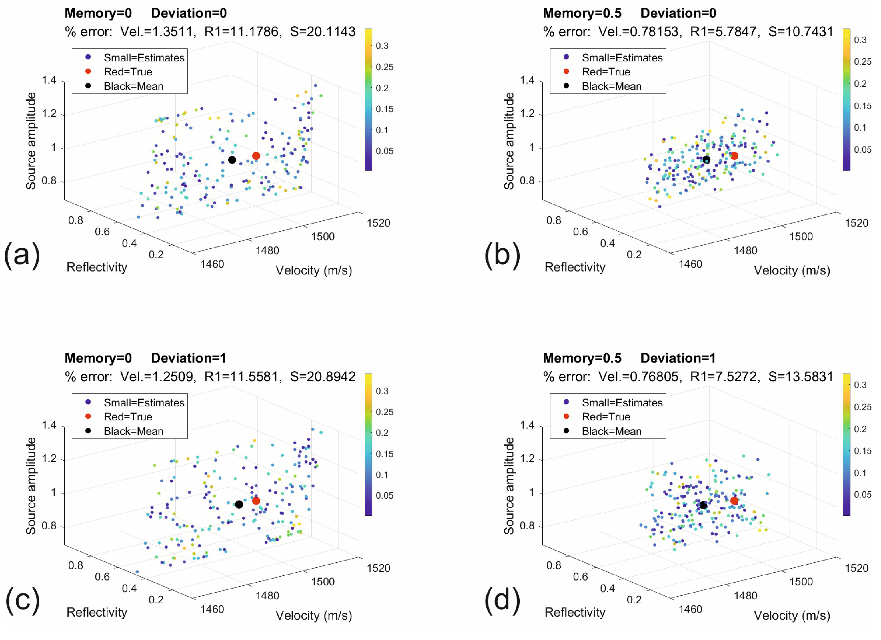
Figure 3.
Synthetic Earth model composed of a water layer overlying some sediments: P velocity (a) and density (b).
Figure 3.
Synthetic Earth model composed of a water layer overlying some sediments: P velocity (a) and density (b).
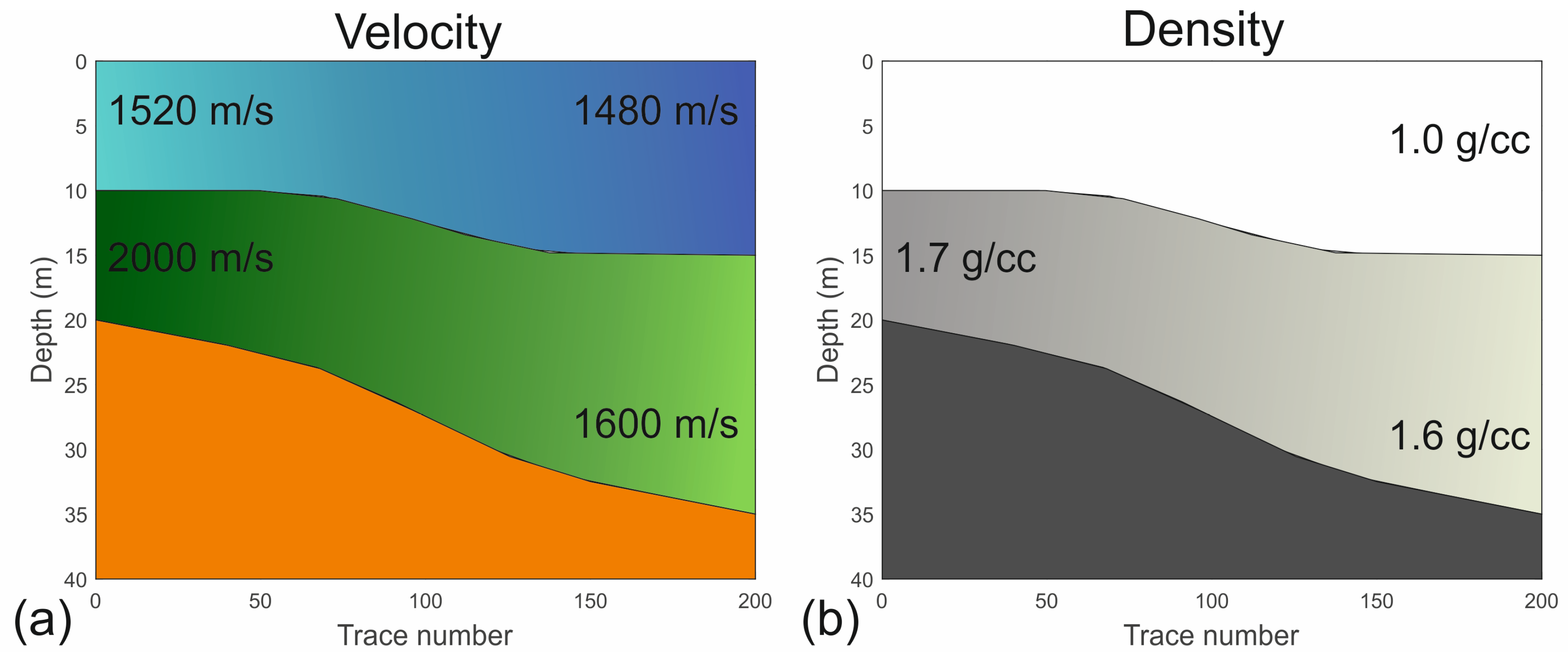
Figure 4.
Two views of the 3D space of solutions obtained by inverting a profile over the model in Figure 3. The red dots represent the true solution, while the others are the estimated solutions, color-coded according to the deviation of the amplitudes used for the inversion at that point. Dark blue color represents no deviation, while yellow is associated with a high deviation, which indicates mostly noisier amplitudes. The color bar on the right side quantifies visually the deviation of each point in the plot.
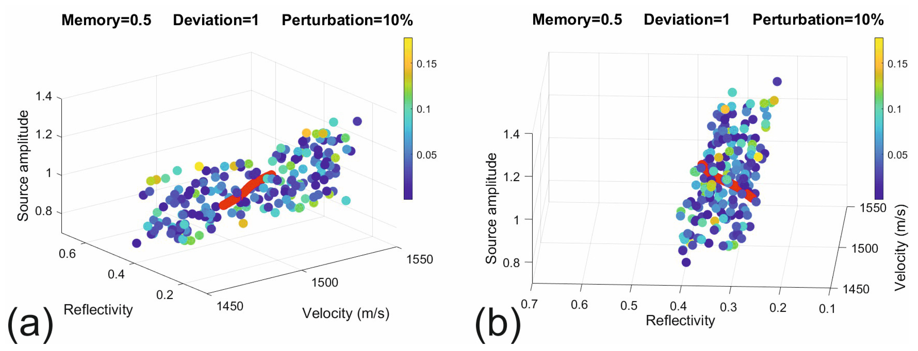
Figure 5.
Estimated model parameters (blue line) and actual ones of the Earth model (red line): reflectivity (a), sea water velocity (b), acoustic impedance of the sediments (c), and their density (d). The green lines in (c,d) represent the smoothed curves obtained by applying a 15-element moving-average filter.
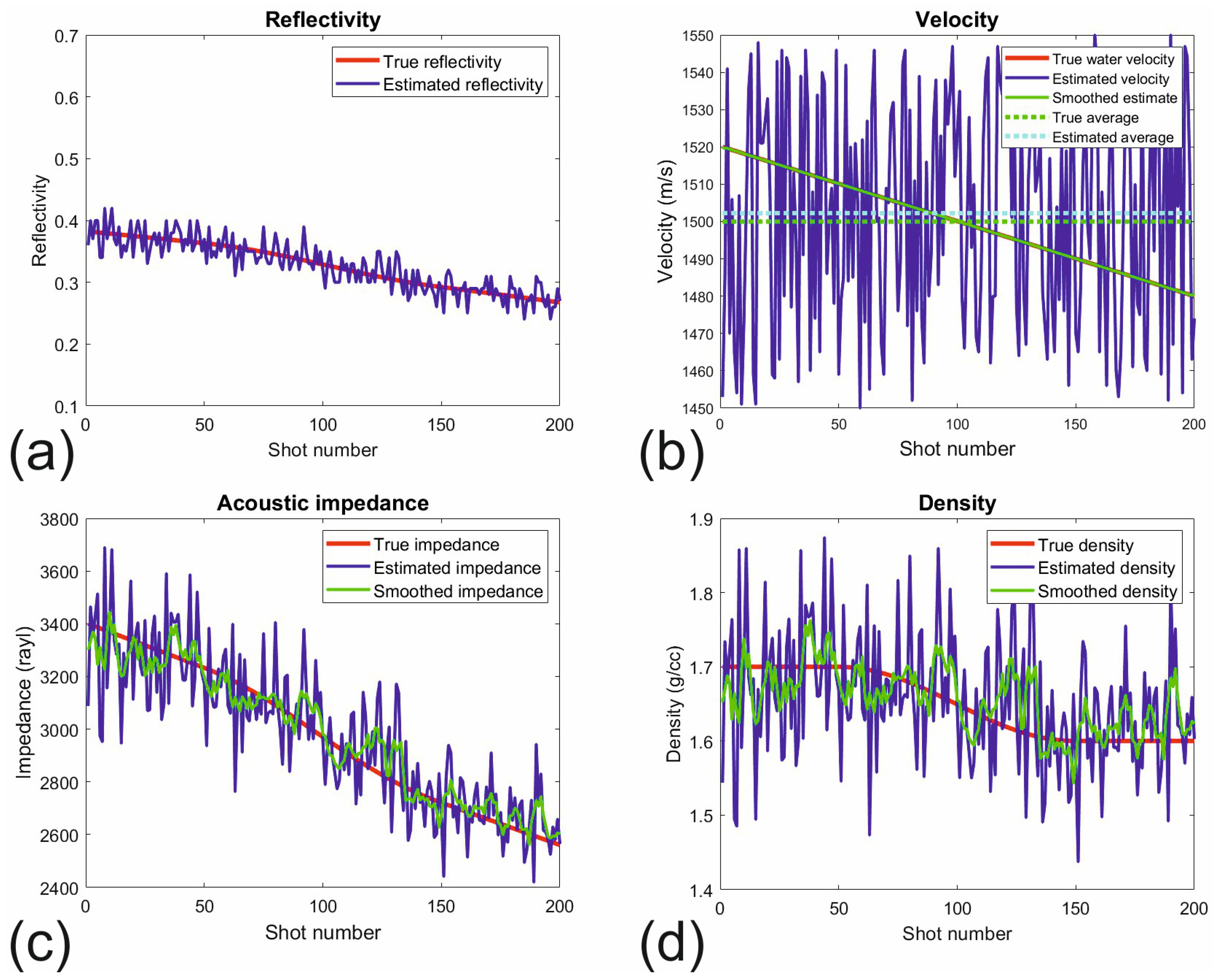
Figure 6.
Estimated model parameters (blue line) and actual ones of the Earth model (red line), obtained by using the true velocity instead of the estimated one: reflectivity (a), sea water velocity (b), acoustic impedance of the sediments (c), and their density (d). The green lines in (c,d) represent the smoothed curves obtained by applying a 15-element moving-average filter.

Figure 7.
Recording geometry for the Boomer survey.
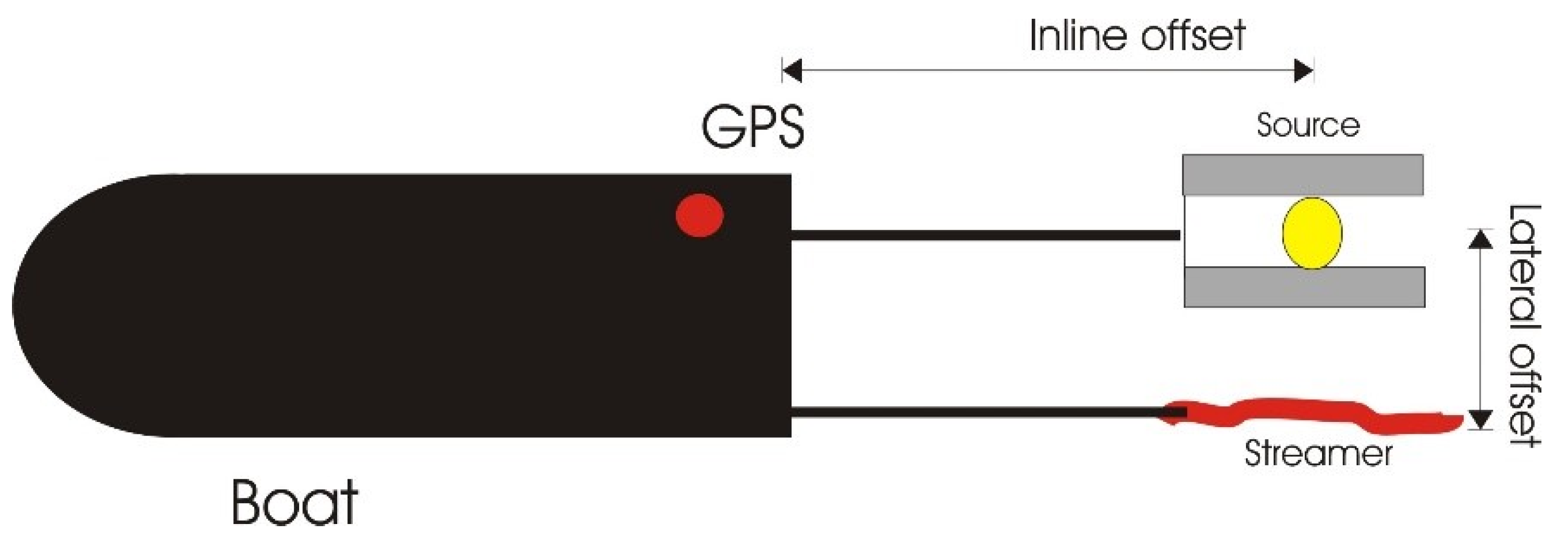
Figure 8.
Parts of the recording system used for the survey: energy source (top) and Boomer plate (bottom).
Figure 8.
Parts of the recording system used for the survey: energy source (top) and Boomer plate (bottom).
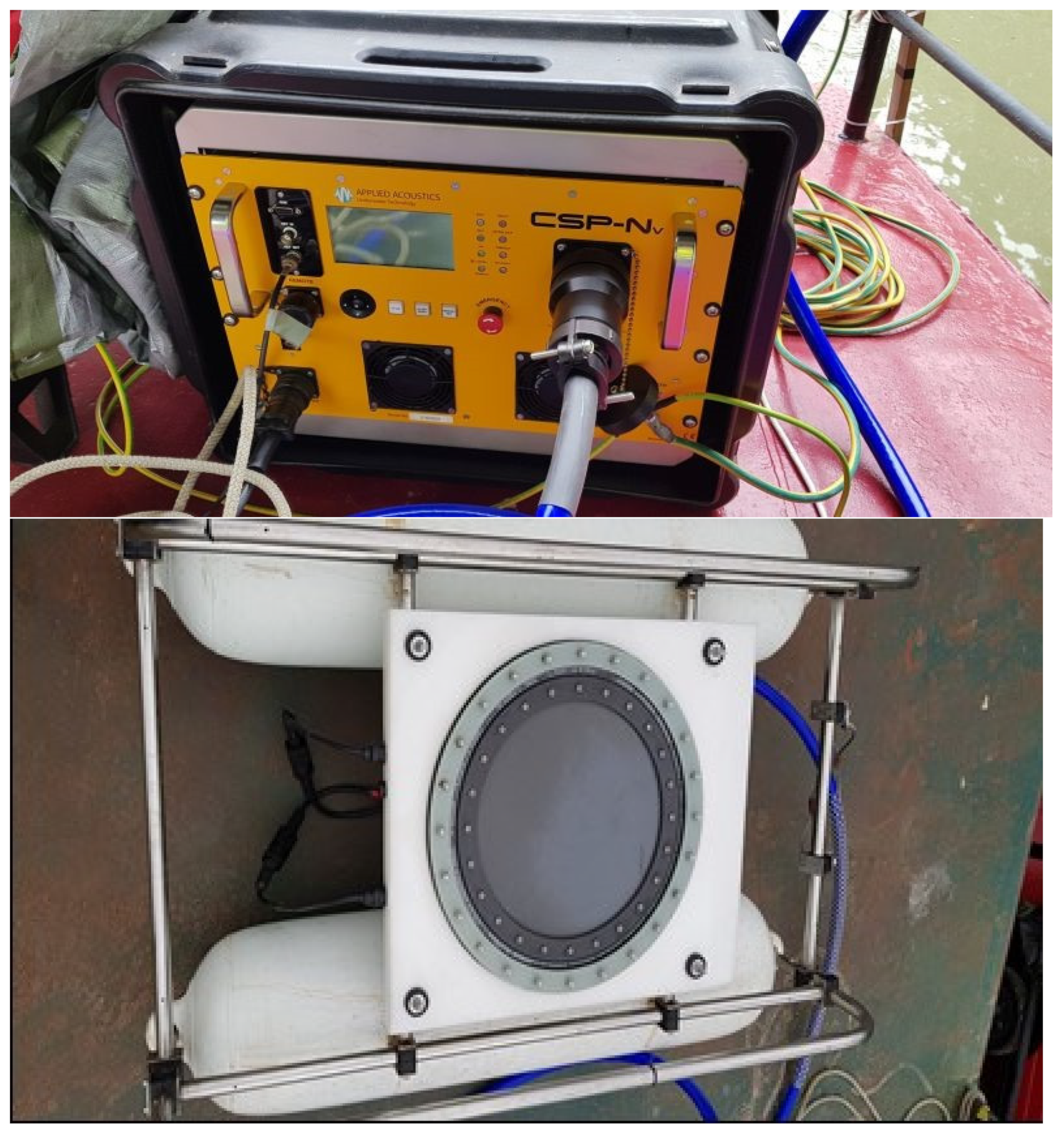
Figure 9.
Seismic section acquired by a Boomer system offshore the Asinara Island. We picked the sea floor (red line), as well as its first (green line) and second multiple (blue line), reverberating between the sea floor and its surface.
Figure 9.
Seismic section acquired by a Boomer system offshore the Asinara Island. We picked the sea floor (red line), as well as its first (green line) and second multiple (blue line), reverberating between the sea floor and its surface.
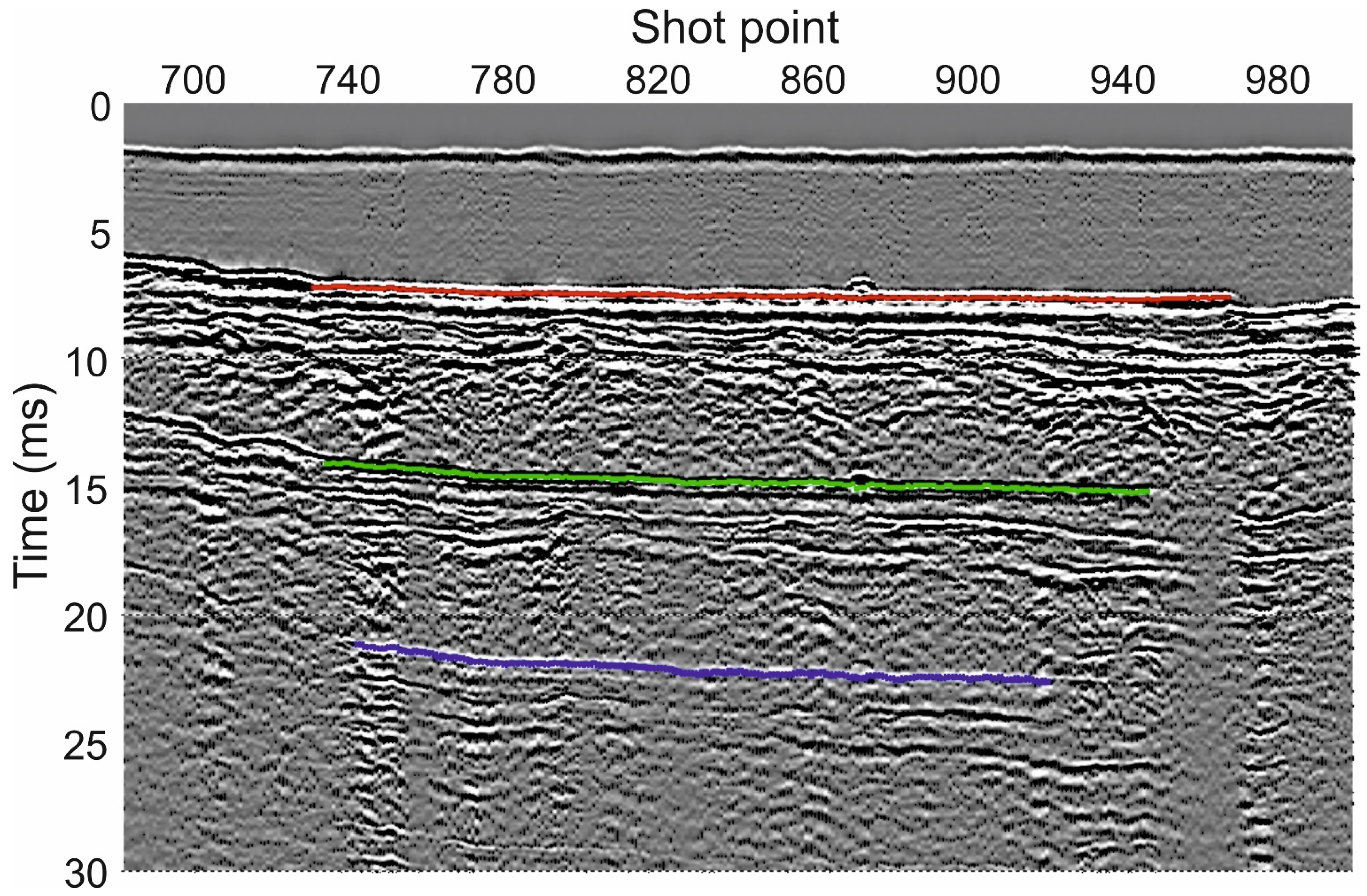
Figure 10.
Estimated reflectivity for the seafloor picked in Figure 7 (red line) using also the amplitudes of the multiples (green and blue lines). The dispersion of the estimated values at each trace decreases when the memory factor increases from 0 (A) to 0.5 (B) and to 0.9 (C). The deviation of the experimental points from the estimated fit is color-coded in the circle from blue (no deviation) to yellow (maximum deviation).
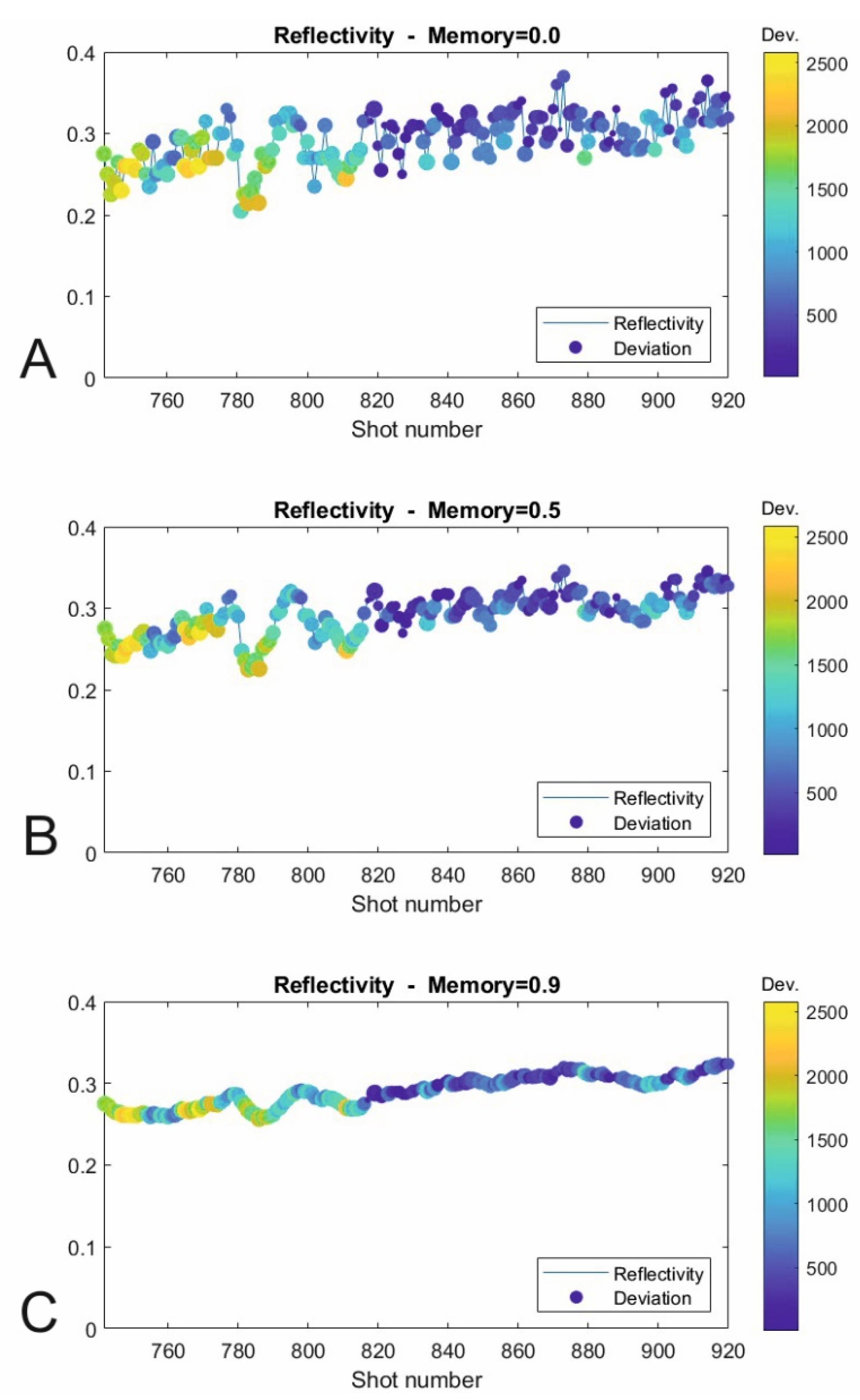
Figure 11.
Estimated density (yellow line) based on the reflectivity as computed in Figure 8, assuming three different velocities for the shallow sediments: 1800 m/s (A), 2000 m/s (B), and 2200 m/s (C). The differences among the three cases are small.
Figure 11.
Estimated density (yellow line) based on the reflectivity as computed in Figure 8, assuming three different velocities for the shallow sediments: 1800 m/s (A), 2000 m/s (B), and 2200 m/s (C). The differences among the three cases are small.


Table 1.
Amplitude of multiples with several bounces between sea floor and surface.
| Two-way time | 0 | ∆t | 2 ∆t | 3 ∆t | 4 ∆t |
| Amplitude | 1 | R1 | R12 R0 | R13 R02 | R14 R03 |
| Multiple order | 0 | 1 | 2 | 3 | 4 |
Table 2.
Main recording parameters for the marine survey off Asinara Island.
| Source type | Boomer, model AAE301 |
| Manufacturer | Applied Acoustics Engineering |
| Recording system | SB-logger |
| Frequency range | 0.4–6 kHz |
| In-line offset source-receiver | About 3 m |
| Lateral offset source-receiver | About 1 m |
| Navigation speed | 3.5–4 knots |
| Recorded shots | 300 |
| Shooting interval | 3 per second |
| Distance between shots | 0.6–0.7 m |
| Sampling interval | 50 microseconds |
| Recording duration | 200 milliseconds |
Disclaimer/Publisher’s Note: The statements, opinions and data contained in all publications are solely those of the individual author(s) and contributor(s) and not of MDPI and/or the editor(s). MDPI and/or the editor(s) disclaim responsibility for any injury to people or property resulting from any ideas, methods, instructions or products referred to in the content. |
© 2023 by the authors. Licensee MDPI, Basel, Switzerland. This article is an open access article distributed under the terms and conditions of the Creative Commons Attribution (CC BY) license (https://creativecommons.org/licenses/by/4.0/).
Share and Cite
MDPI and ACS Style
Vesnaver, A.; Baradello, L. Sea Floor Characterization by Multiples’ Amplitudes in Monochannel Surveys. J. Mar. Sci. Eng. 2023, 11, 1662. https://doi.org/10.3390/jmse11091662
AMA Style
Vesnaver A, Baradello L. Sea Floor Characterization by Multiples’ Amplitudes in Monochannel Surveys. Journal of Marine Science and Engineering. 2023; 11(9):1662. https://doi.org/10.3390/jmse11091662
Chicago/Turabian StyleVesnaver, Aldo, and Luca Baradello. 2023. "Sea Floor Characterization by Multiples’ Amplitudes in Monochannel Surveys" Journal of Marine Science and Engineering 11, no. 9: 1662. https://doi.org/10.3390/jmse11091662
Note that from the first issue of 2016, this journal uses article numbers instead of page numbers. See further details here.