
Laboratory Investigations of Iceberg Melting under Wave Conditions in Sea Water


Arctic Technology Department, The University Centre in Svalbard, 9171 Svalbard, Norway
*
Author to whom correspondence should be addressed.
J. Mar. Sci. Eng. 2024, 12(3), 501; https://doi.org/10.3390/jmse12030501
Submission received: 19 February 2024
/
Revised: 11 March 2024
/
Accepted: 13 March 2024
/
Published: 18 March 2024
(This article belongs to the Special Issue Recent Research on the Measurement and Modeling of Sea Ice)
Abstract
:Changes in the masses of icebergs due to deterioration processes affect the drift of icebergs and should be taken into account when assessing iceberg risks in the areas of offshore development. In 2022 and 2023, eight laboratory experiments were carried out in the wave tank of the University Centre in Svalbard to study the melting of icebergs in sea water under calm and rough conditions. In the experiments, the water temperatures varied from to . Cylindrical iceberg models were made from columnar ice cores with a diameter of 24 cm. In one experiment, the iceberg model was protected on the sides with plastic fencing to investigate the iceberg’s protection from melting when towed to deliver fresh water. The iceberg masses, water temperatures, and ice temperatures were measured in the experiments. The water velocity near the iceberg models was measured with an acoustic Doppler velocimeter. During the experiments, time-lapse cameras were used to describe the shapes and measure the vertical dimensions of the icebergs. Using experimental data, we calculated the horizontal dimensions of icebergs, latent heat fluxes, conductive heat fluxes inside the iceberg models, and turbulent heat fluxes in water as a function of time. We discovered the influence of surface waves and water mixing on the melt rates and found a significant reduction in the melt rates due to the lateral protection of the iceberg model using a plastic barrier. Based on the experimental data obtained, the ratio of the rates of lateral and bottom melting of the icebergs and lateral melting of the icebergs under wave conditions was parametrized depending on the wave frequency.
1. Introduction
In the Barents Sea, icebergs are formed as a result of the calving of outflow glaciers of Spitsbergen, Franz Josef Land, and Novaya Zemlya [1,2,3]. The rate of iceberg formation and the sizes of icebergs are determined by the thickness and dynamics of the glaciers, as well as the seabed bathymetry calving areas [4]. The average sizes of icebergs in the Barents Sea were characterized by a height above sea level of 11 m, a length at the water level of 140 m, a width at the water level of 70 m, and a draft of 50 m. The average mass of an iceberg was estimated at 927 thousand tons [5]. The general direction of the iceberg drift corresponds to the direction of the surface currents. This means that most of the icebergs formed by the outflow glaciers of Spitsbergen and Franz Josef Land drift southwest following the East Spitsbergen Current, and some icebergs may drift into the central regions of the Barents Sea under the influence of wind, waves, and drift ice.
The actual trajectories of drifting ice and icebergs in the Barents Sea have a complex shape, with numerous loops and corner points due to the combined influence of inertial forces, tidal currents, and winds [6]. Iceberg trajectories were reconstructed using geolocation data transmitted by buoys installed on icebergs [7,8,9]. Typically, the lifetime of a buoy on an iceberg in the Barents Sea does not exceed one month. To a certain extent, this is due to deterioration of icebergs, affecting the positions of the buoys on icebergs. The deterioration of icebergs leads to a decrease in their mass and changes in the shape and position of the icebergs. These processes change the balance of inertial and drag forces acting on icebergs, and in turn, affect the drift of icebergs.
Estimates of the appearances of icebergs in various regions of the Arctic and Antarctic are necessary for climate modeling [10], freshwater supply [11], offshore development [12], and shipping [12,13]. Numerical simulations of iceberg drift have been performed to calculate the probability of iceberg appearances in specific regions [14,15,16,17,18,19]. The research was based on a numerical analysis of momentum balance equations describing the drift of icebergs. Changes in the masses of icebergs due to deterioration processes affected the drift of icebergs.
Several physical processes contributing to the deterioration of icebergs have been considered in the scientific literature, including the bending failure of icebergs [20,21], surface [22], bottom [23], and lateral [24] melting of icebergs, and wave erosion [25,26]. Bending failure is the most important factor influencing the splitting of large tabular icebergs calved from glaciers of the Antarctic and Greenland into smaller patterns. The size of icebergs in the Barents Sea is much smaller than in Antarctica or near Greenland. Therefore, we hypothesize that bending failure is a relatively rare phenomenon, and the main physical mechanism of iceberg deterioration in the Barents Sea is attributed to melting.
Crawford et al. [22] studied the surface ablation of an ice island that broke away on 5 August 2010 from the Petermann Glacier in northwest Greenland (81° N, 61° W). The estimated surface ablation rate was approximately 1 m per month (August 2011) or 1.4 mm/h. The rate of surface ablation of the glaciers in this region is approximately the same. Similar estimates were obtained for Spitsbergen glaciers [27].
The bottom melting of icebergs was studied to estimate the potential loss of ice mass when icebergs are towed from Antarctica to provide a source of fresh water in arid regions [23]. Using the theory of a turbulent boundary layer in the water flow near a semi-infinite plate, the rate of bottom melting was estimated [28]. The melting rate was obtained as proportional to , where and are the velocities of the iceberg and water, and is the difference in the water and ice temperatures. The use of this formula causes problems when the iceberg drifts with surrounding water. In this case, is determined by the movement of melt water in the boundary layer and must be found from the solution of the boundary layer problem. The rocking of icebergs caused by waves also affects the movement of water relative to the surface of the icebergs.
Russell-Head [29] investigated the melting of iceberg models in calm water of different temperatures and salinities. Most of the experiments were carried out at water temperatures above 3 °C. The effect of salinity on the melt rate was found to be negligible for icebergs floating in water with a salinity ranging from 17.5 ppt and 35 ppt. Daley and Vetch [13] studied the melting of iceberg models in calm water and under rough conditions. The water temperature was 15–16 °C. It has been found that the rate of the mass loss of icebergs in calm water and in rough water conditions is the same. The empirical formulas of El-Tahan et al. [26] were derived from observations of large icebergs in Antarctica.
Josberger [30] and White et al. [25] studied the effect of notch formation in the iceberg wall at the waterline caused by waves. Josberger [30] conducted the only wave erosion experiment with a wave height of 5 cm and a wave period of 0.4 s in water with a temperature of 4 °C. White et al. [25] reported the results of two experiments on melting, floating ice blocks in a circular wave tank filled with water with a temperature of 13.5 °C. Using the Reynolds analogy, White et al. [25] derived a formula that describes the melting rate at the waterline depending on the wave height, wave period, and temperatures of water and ice. White et al. [25] reported the formation of ripples on the surface of submerged ice. Josberger and Martin [31] described the formation of cusps on a vertical ice wall melting in salt water with a temperature above 25 °C. A scallop-shaped structure was observed on the bottom surface of floating ice and on the surfaces of icebergs under natural conditions [32] and in laboratory experiments [33].
This paper describes the results of laboratory experiments on the melting of iceberg models floating in sea water under rough conditions. In accordance with the geometrical similarity, the sizes of the iceberg models and wave frequencies correspond to the sizes of icebergs and the frequencies of swell and wind waves in the Barents Sea. The experiments were carried out in a cold laboratory at the University Centre in Svalbard, with water temperatures below 2 °C. This paper consists of an Introduction (Section 1) and six sections describing the organization of the experiments (Section 2), geometrical and physical scaling (Section 3), data processing (Section 4), obtained results (Section 5), the Discussion (Section 6), and Conclusions (Section 7). Section 5 includes five subsections describing the data obtained on the evolution of icebergs masses and shapes, ice and water temperatures, and heat fluxes in water and ice.
2. Laboratory Experiment
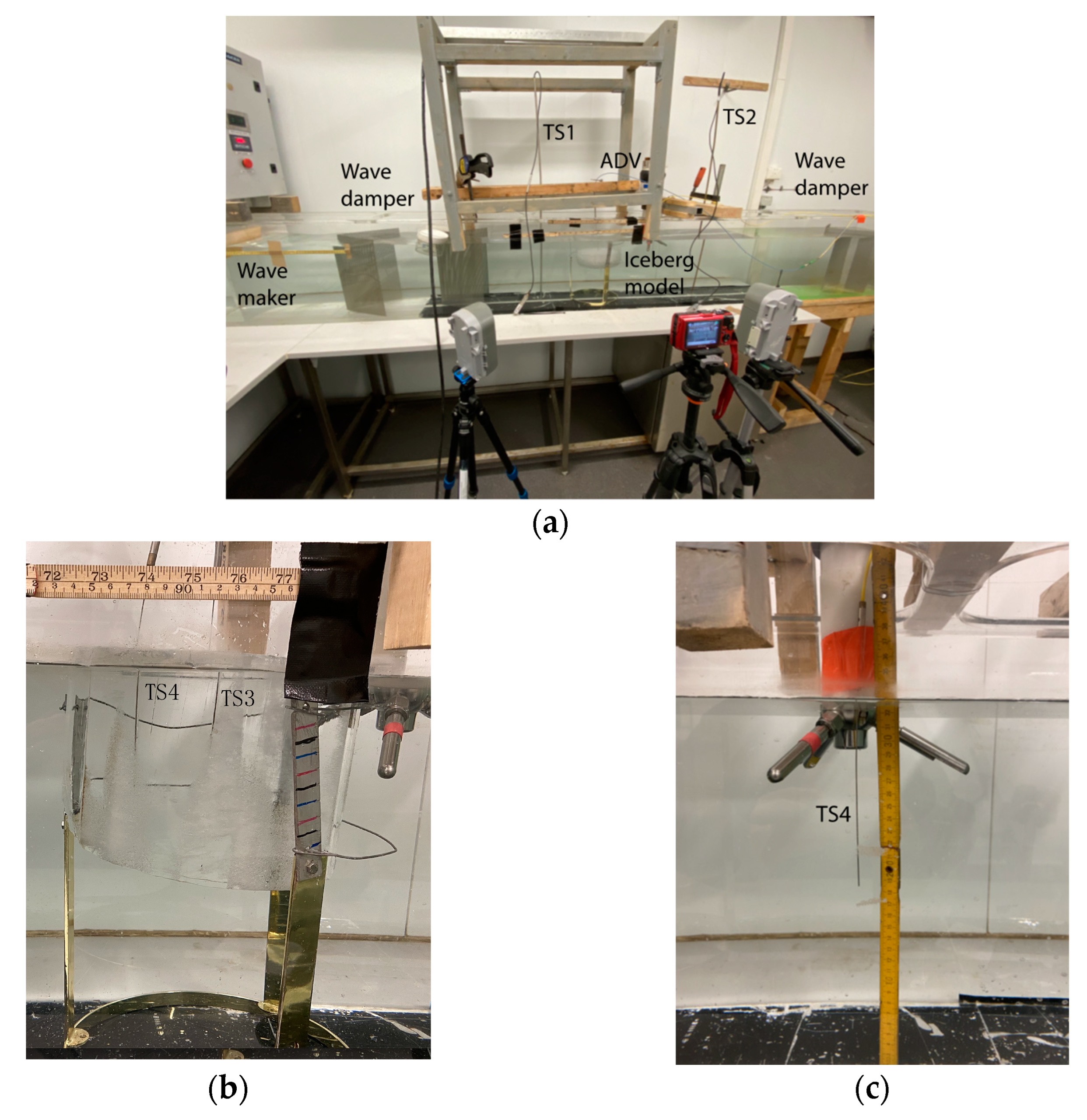
Eight laboratory experiments (1–8) were carried out in the cold laboratory of the University Centre in Svalbard in December 2022 and February 2023. Figure 1 shows the organization of the experiments and installation of equipment. The experiments were carried out in an acrylic wave tank that was 3.5 m long and 30 cm wide and was filled with sea water with a salinity of 33.5 ppt. The water depth in the tank was 32 cm. Blocks of columnar freshwater ice of a cylindrical shape were made from the ice cores of lake ice to model icebergs. The height and diameter of the ice blocks were about 15 cm and 24 cm, respectively. The surfaces of some iceberg models were chipped. The iceberg models were placed inside a metal-wire frame that prevented them from drifting along the tank, but did not limit their heave, roll, pitch, and yaw within the frame. Vertical frame elements were marked to measure the vertical dimensions of floating icebergs using video recordings and photographs, which were taken during the experiments. Horizontal and vertical length scales were also glued to the tank wall.
To create waves in the tank, a wedge-shaped wavemaker was used, crossing the water surface, and cyclically moving in the vertical direction. The frequency of movement of the wavemaker varied in the range of 1–3 Hz. Wave dampers (perforated metal plates and floating plastic boxes filled with water) were used to reduce the amplitude of waves near the iceberg and reduce the amplitude of waves reflected from the tank wall. The amplitude, frequency, and wavelength were measured using video camera recordings.
The water temperature was measured using two temperature strings, TS1 and TS2 Geoprecision (Ettlingen, Germany), installed vertically in the wave tank in the front and behind the iceberg model for experiments 1–4. For experiments 5–8, only temperature string TS1 was installed. Temperature measurements were carried out with a spatial resolution of 5 cm and a temporal resolution of 1 min (Figure 1a). The accuracy and resolution of TS1 and TS2 were 0.1 °C and 0.01 °C, respectively.
For experiments 1–4, a fiber optic temperature string (FBG sensors), TS3 (AOS GmBh, Dresden, Germany), was installed at the middles of icebergs to measure the vertical profile of the ice temperature (Figure 1b). A similar temperature string, TS4, was installed, along with an acoustic Doppler velocimeter (Sontek ADV Hydra 5 MHz, San Diego, CA, USA) to measure the temperature and calculate the turbulent heat flux (Figure 1c). The sampling interval was programmed to 1 Hz for ice temperature measurements and 200 Hz for heat flux calculations.
FBG sensors provide measurements with a formal resolution of 0.012 °C. The AOS GmBh limits the accuracy and resolution of the temperature measurements with FBG sensors to 0.4 °C and 0.08 °C, respectively, due to system noise and environmental influences. The length of the fiber Bragg grating, with 20,000 cells representing each FBG sensor, is 1 cm. It is burned by two interfering laser beams in an optical fiber with a diameter of . An optical fiber with 12 FBG sensors is placed in a metal tube with a diameter of 1 mm. The thermal inertia of FBG sensors is very small compared to other types of temperature sensors. FBG sensors were calibrated in a mixture of ice and fresh water with a stable temperature of 0 °C. The moving average procedure was applied to the row data to exclude a noise caused by the short response time of FBG sensors.
For experiments 5–8, the temperature string TS3 was installed in the middles of icebergs, and the temperature string TS4 was installed at a distance of 7–8 cm from TS3 at the walls of the icebergs (Figure 1b and Figure 2a). The distance between points A1 and B1 as well as points A2 and B2 in Figure 2a was 7–8 cm. Temperature strings were placed in vertical holes with a diameter of 2.5 mm and a length of 10 cm and drilled into the iceberg: the lengths of the segments (A1, A2) and (B1, B2) in Figure 2a were equal to 10 cm. Segments (A1, A2) and (B1, B2) each included 8 temperature sensors. Four temperature sensors were in the air at 1, 2, 3, and 4 cm distances above the surfaces of the icebergs. Temperature sensor 1 measured the temperature 8 cm below the iceberg’s surface, and temperature sensor 12 measured the temperature 4 cm above the iceberg’s surface. The positions of the temperature sensors are indicated by the horizontal strips in Figure 2a.
The ADV sampling rate was programmed to 25 Hz. The measurements were carried out in bursts with a 20 min burst interval. In each burst, the ADV collected 20,000 water velocity samples over 800 s. Figure 2b shows the sampling locations of the ADV and TS4 relative to the iceberg model. The velocity range index ADV was assigned a value 0, corresponding to a velocity range of cm/s. The probe accuracy is of the measured speed of mm/s. ADV seeding material was added to the water to ensure that the correlation of the recorded data was greater than 70%. ADV measurements were carried out in intervals of turbulent measurements (ITMs). During these intervals, TS4 sampled at a 200 kHz frequency, and TS3 did not operate.
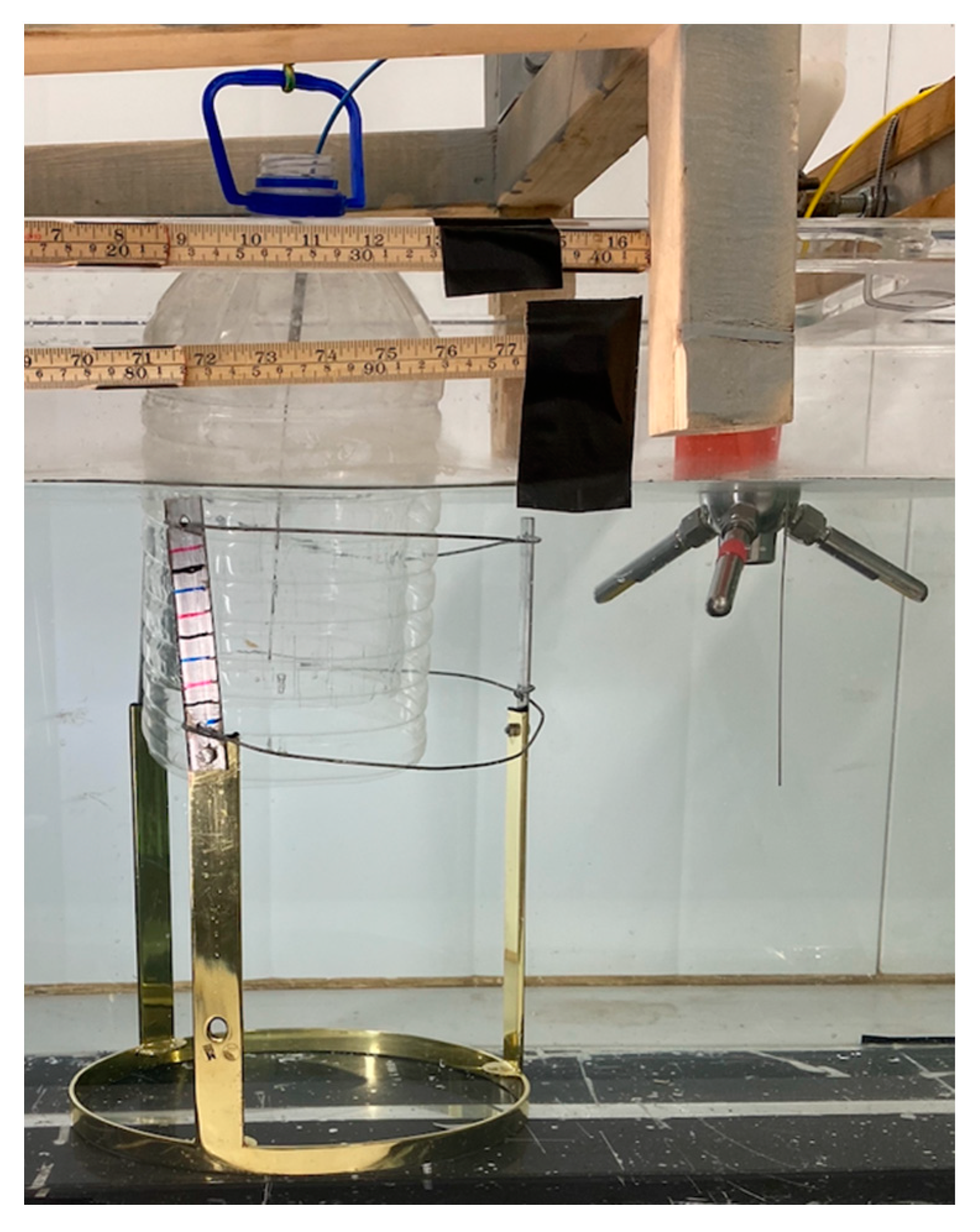
The experiment durations (ED), wave amplitudes (), and wave frequencies () are given in Table 1. The wave amplitude was measured from video recordings at a distance of 20 cm from the icebergs. At the water–ice boundary, the amplitudes of water movement were greater. The values in Table 1 indicate representative wave amplitudes in the tests. Experiment 4 was conducted using an iceberg model that was protected on the sides by a plastic barrier made from a plastic bottle (Figure 3). The bottom of the bottle was cut off, and the iceberg was in direct contact with the sea water below. The space between the ice and the wall of the bottle, which was 1–2 cm wide, was also filled with a mixture of sea water and melt water. The purpose of the experiment was to investigate a way to reduce the melting of icebergs during towing [11].
3. Scaling
The diameter of an iceberg is considered as a representative horizontal scale. The geometric scaling factor is the ratio of the natural-scale iceberg diameter () to the model-scale iceberg diameter (). The eigen frequency of the heave oscillations of a cylindrical iceberg is calculated using the formula
where and are the water and ice densities, and are the vertical dimension and the radius of the iceberg, is the gravity acceleration, and is the added mass coefficient [34,35]. Assuming kg/m3, kg/m3, cm, and cm, we find rad/s, and the period of natural oscillation is s. It is very close to the period 0.96 s for heave oscillations of iceberg models measured in the experiments.
We assume that the scaling factor changes in the range . This corresponds to the vertical dimensions of full-scale icebergs (from 12 m to 60 m), with the vertical height for an iceberg model of 15 cm. Accordingly, the radii of full-scale icebergs vary in the range from 10 m to 50 m, when the radius of an iceberg model is 12 cm. The full-scale dimensions correspond to the typical sizes of icebergs in the Barents Sea.
From (1), it follows that the eigen frequency of the heave oscillations of the full-scale cylindrical iceberg is calculated using the formula
The wave length is calculated from the dispersion equation
where the wave number is , and is the water depth. The wave frequency in the experiments changed according to Table 1, in the range rad/s. The wave frequencies were higher than the eigen frequencies of the iceberg models in the experiments. Assuming m, we find that the wave numbers were in the range m−1 (Table 1), and the wave lengths were in the range cm. The wave numbers satisfied the inequality > 2, allowing us to assume . Thus, the deep water approximation is valid for describing waves in the experiments.
The frequency of waves and the period of waves at the full scale and the model scale are related by the formulas
Figure 4 shows the full-scale periods and amplitudes of waves calculated with the model wave periods measured in the experiments versus the geometrical scaling factor (Table 1). Full-scale periods varying from 4 s to 15 s correspond to periods of wind waves and swell. Full-scale amplitudes are within the typical values of swell and wind wave amplitudes in the Barents Sea [15].
The time for temperature equalization in an ice body with fixed boundaries is determined using the formula
where kJ/(kg ) is the specific heat capacity of ice, W/(m ) is the thermal conductivity of ice, is the body diameter, and is a dimensionless coefficient depending on the body shape and boundary conditions [36]. The coefficient when the body is a cube with side and a fixed temperature on the faces. The full-scale time of temperature equalization is calculated with the formula .
The representative iceberg melting time () spent for the melting of 10% of the iceberg mass is calculated using the formula
From the energy balance, it follows with
where kJ/kg is the latent heat from ice fusion, is the mean heat flux to the ice–water interface, and is the area of the submerged surface of the iceberg. The heat flux is the sum of the heat fluxes from water and from ice to the interface. Assuming that the full-scale mass and area of the submerged surface of the iceberg are scaled to the model quantities as and , we found , where is the heat flux scale factor.
The conductive horizontal heat flux from the iceberg to the ice–water interface is estimated with the formula
where is the interface temperature, and is the ice temperature in the iceberg center. The inequality is valid for on a laboratory scale. Assuming similar values of in the laboratory experiment and in the full-scale study we found that . In the full-scale study , and the inequality is valid in any time if .
The temperature can be higher than the freezing point of the ambient sea water, since the salinity of the melt water is less than the salinity of the ambient water. Neshyba and Josberger [36] considered the thermal driving for the melting of a vertical ice wall using
where is the ambient water temperature.
The heat flux to the iceberg surface depends on the type of water movement near the iceberg surface [31]. In stagnant water, the convective flow near a vertical ice wall is laminar near the bottom edge of the wall and becomes turbulent at a distance of 20 cm from the edge. Neshyba and Josberger [24] estimated the average melting rate over the wall height using the formula
where is the wall height above the transition point from the laminar to turbulent boundary layer. The term sets the heat flux scale factor as .
Wells and Worster [37] and Kerr and McConnochie [38] considered the dissolution and melting of a vertical ice wall caused by the influence of salt water. Dissolution is characterized by a discontinuity of salinity at the ice–water interface. In our experiments, the ice salinity was zero, and the ice temperature was below zero even after temperature equalization. It indicates a nonzero water salinity at the interface. Therefore, in our experiments, the ice surface dissolved. Thermal driving for the dissolution of the vertical wall equals the difference between the salinities of the ambient water () and the water at the interface ():
The salinities of the ambient water () and the water at the interface () are expressed by the formulas [39]
The salinity of the ambient water in the experiments was ppt, and the freezing point was .
The seawater density is expressed by the formula [37]
where is the ambient water density. Formula (13) captures the dominant buoyancy driving the flow for ice and seawater systems.
A self-similar solution describing the dissolution of the vertical ice wall in a laminar flow leads to the melting rate [38]
where m2/s is the compositional diffusivity, and m2/s is the kinematic viscosity of the sea water. Using Formula (12), we modify Formula (14) to
where thermal driving is
Assuming , we find m5/4/(day 5/4). The heat flux scale coefficient equals .
Kerr and McConnochie [38] adopted the formula , derived for a turbulent thermal boundary layer with , to describe dissolution [40]. The dissolution rate was calculated with the formula
Using Formulas (12) and (13), we modify Formula (17) to
Assuming , we estimate m/(day 4/3). Formulas (17) and (18) do not support any scale effect, and .
White et al. [25] used Reynolds analogy-derived formulas to determine the melting rate caused by the wave erosion of fixed iceberg at the waterline:
where and are, respectively, the wave amplitude and wave frequency, is the wave’s Reynolds number, and is roughness height. Formulas (19) and (20) are valid, respectively, for the smooth () and rough () surfaces of ice.
The heat flux scale coefficient equals according to Formula (19), and according to Formula (20), if the ratio is the same in the full and model scales. Formulas (10), (14) and (15) support a decreasing dissolution rate with an increasing geometrical scale , while Formulas (19) and (20) predict an increasing wave-induced melting rate with an increasing geometrical scale .
We assume the pitch and heave motions of floating icebergs caused by waves with amplitudes similar to the wave amplitudes. In this case, Formulas (19) and (20) are modified in the following way:
where the first summand describes the melting rate caused by the pitch and heave of the iceberg, and the second summand describes the melting rate due to the wave action itself. Empirical coefficients describe the dependence of the pitch and heave velocity amplitudes on the wave amplitude and frequency. Symbol 〈 〉 means the averaging over the iceberg draft , which is calculated using the formula
where the factor describes the dependence of the wave-induced water velocities on the depth in deep water ( 2).
The calculation of integral (22) leads to the formulas
Coefficients and reach a maximal value of 1.0 at , and monotonically approach 0 at . Finally, the wave-induced melting rate of a floating iceberg is expressed by the formula
with the wave correction factor depending on the wave amplitude, wave frequency, and parameters characterizing the response of the iceberg on the wave action.
4. Data Processing
4.1. Iceberg Dimensions
An accurate reconstruction of the 3D shape of icebergs was not possible with time-lapse images. Therefore, we approximated the icebergs using cylinders of an equivalent mass. The iceberg mass was measured during the experiments. Time-lapse images were used to measure the vertical dimension of the iceberg, , during the experiments. Markers placed over each centimeter on the metal frame were well visible on the images (Figure 1). Finally, the iceberg radius was calculated using the formula
4.2. Turbulence Measurements
The turbulent heat flux , kinetic energy of velocity fluctuations (), and standard deviation () of temperature fluctuations () were calculated using the formulas
where is the water velocity measured using the ADV in the point shown in Figure 2, is the water temperature measured using the temperature sensor of the TS4 string closest to the point of the velocity measurement, and are the mean values averaged over an 800 s interval, and are the fluctuations in the velocity and temperature, and kJ/(kg ) is the specific heat capacity of water. High frequency measurements of the water temperature and velocity were carried out in turbulent measurement intervals (ITMs), which are specified further.
4.3. Heat Fluxes to Iceberg Surfaces
Heat fluxes to the unit areas of the submerged surface and bottom surface of a cylindrical iceberg are calculated with the formulas
The area of the submerged surface of a cylindrical iceberg is equal to the sum of the areas of the lateral and bottom surfaces of the iceberg
Here, and are, respectively, the areas of the lateral and bottom surfaces of the iceberg.
The heat flux to the lateral surface of a cylindrical iceberg () is calculated as follows:
Furthermore, the heat fluxes , , and are called the latent heat fluxes.
5. Results
5.1. Water Temperature
The water temperature in the experiments changed because of the convection of water in the tank and changes in the air temperature. Figure 5 shows the depth-averaged water temperatures versus the time in different experiments. In experiments 1–4, temperature fluctuations of about 1 °C were recorded. In experiments 5–8, temperatures fluctuations were smaller, but the durations of the experiments were shorter. The mean water temperatures for the experiments are given in Table 2. The mean water temperatures measured using TS1 and TS2 in experiments 1–4 are shown over a forward slash in Table 2. There is temperature gradient along the tank of about 0.4 °C per 1 m, supported by the air temperature gradient in the room.
5.2. Icebergs Masses and Shapes
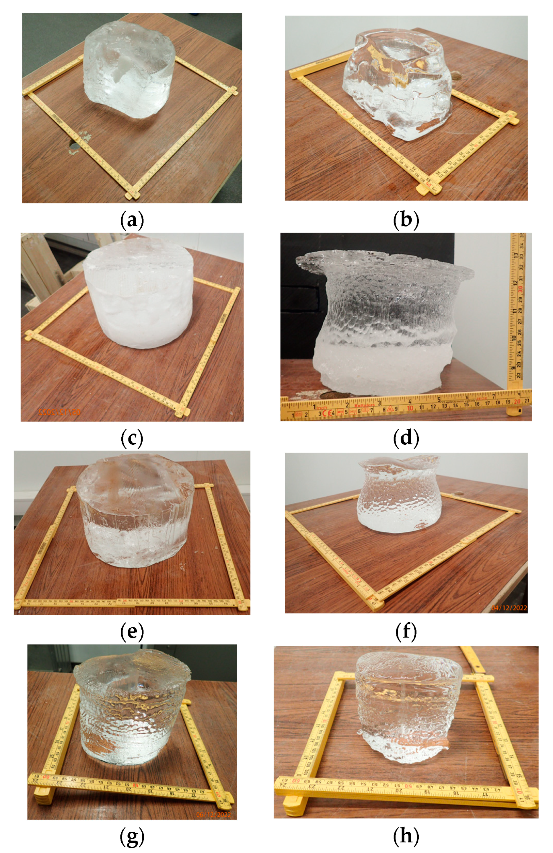
Photographs of the iceberg models before and after experiments 1–4 are shown in Figure 6. In experiment 1, the iceberg model melted in calm water. In experiment 1, the iceberg’s surface remained smooth, but the iceberg’s lateral surface became conical and tapered with time (Figure 6a,b). In all experiments with waves (2–8), we observed the formation of scallops on the submerged surfaces of the icebergs (Figure 6d,f,h). In experiments 2, 3 (Figure 6d,f), and 5–8, the scallops were distributed evenly over the icebergs’ surfaces and had similar dimensions in different directions. In experiment 4, the scallops were slightly elongated in the horizontal direction and grouped in horizontal chains (Figure 6g,h).
The wave-induced motion of the water attenuated at a depth of . This depth was less than 5 cm in experiments 2–4 and increased to 13 cm in experiment 8. In experiment 4, the iceberg surface was protected from the direct wave action by a plastic barrier made from a plastic bottle. The barrier damped the pitch and roll motions of the iceberg more strongly than the heave and yaw motions. Therefore, we assume that the formation of scallops in experiments 2, 3, and 5–8 was caused by the direct wave action as well as by the heave, pitch, roll, and yaw motions of the icebergs relative to the water. In experiment 4, only the heave and yaw of the iceberg affected the scallop formation.
Thin sections of the iceberg surfaces in experiments 3 and 5 are shown in Figure 7. The length of the yellow strip is 5 cm. The representative diameter of the scallops (roughness length ) was about 1 cm, and representative height of scallops (roughness height ) was about 1 mm. According to video recordings, the amplitudes of the iceberg movements () caused by waves were similar to the amplitudes of waves, and the periods of iceberg movements were similar to the periods of waves (Table 1). Thus, the roughness parameter used by White et al. [25] should be replaced with . Assuming mm and mm, we find . Therefore, the iceberg surface should be considered as a rough surface in the experiments.
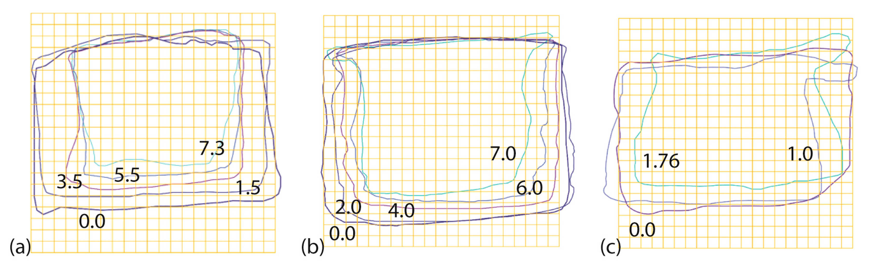
Figure 8 shows the shapes of the vertical cross-sections of the icebergs in experiments 1–3 reconstructed from time-lapse photographs. Time-lapse images were used to reveal the shape changes and particular form appearances. For the measurement of the height, keeping in mind the refraction of light in the water body, we made corrections by measuring the initial and final parameters of the samples on the table/air. The tilt angles of the icebergs in the photographs were determined by the position of the temperature string TS3. The icebergs were then rotated through this angle to compare their shapes at different times. All contours in Figure 8 correspond to the vertical position of TS3. Different contours may correspond to different cross-sections due to the yaw of icebergs. Therefore, it is possible to obtain the vertical dimensions of icebergs versus the time from the contours, but determining the horizontal dimensions of icebergs versus the time from the contours is impossible. It can be seen that the cylindrical approximation of the iceberg shape is reasonable through the experiments.
We did not observe the collapse of the ice caps hanging above the water surface. From Figure 8b,c, it is clear that the volumes of the caps were significantly less than the volume of ice that melted during the experiments. Similar ice caps formed in experiments 5–8 but did not appear in experiments 1 and 4. Directly below the caps, the diameters of the icebergs were smaller than those in bigger depths. Furthermore, this part of the iceberg is called the iceberg waist.
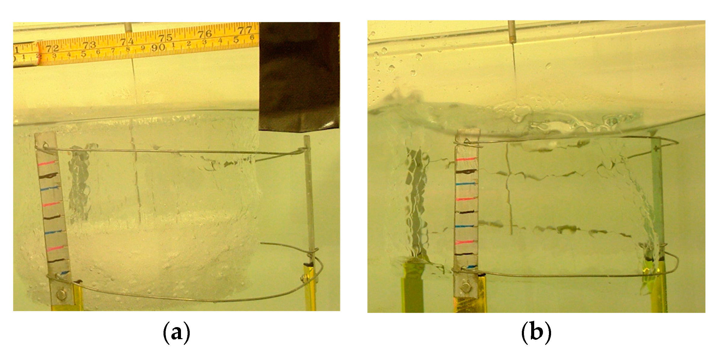
The photographs in Figure 9 illustrate the interactions of waves with icebergs. In experiment 2, the amplitude of the incoming wave was 2 mm at a 20 cm distance from the iceberg. Near the iceberg, the amplitudes of water surface elevation were higher, but water did not appear at the iceberg surface (Figure 9a). A similar type of wave–iceberg interaction occurred in experiments 4–8. In experiment 3, the amplitude of the incoming wave was 7 mm at a 20 cm distance from the iceberg; during the experiment, the wave was systematically observed to roll over the surface of the iceberg (Figure 9b). This significantly affected the shape of the iceberg and increased its melting in the vertical direction.
The iceberg masses and heights measured in experiments 1–8 are given in Table 3 and in Figure 10 versus the time. In all experiments, the masses and heights of the icebergs decreased, and their dependencies on the time were close to linear:
The values of the rates and of the iceberg masses and heights are given in Table 4. Figure 10 shows the dependencies of iceberg radiuses calculated from the equation
The mean rates of the iceberg radiuses are given in Table 4.
5.3. Ice Temperature
Figure 11 shows the ice and air temperatures measured using temperature string TS3, which was installed in the middles of the icebergs in experiments 1, 2, and 4 (Figure 1b and Figure 2a). The temperature data from experiment 3 are not shown, because the temperature was affected by the waves rolling over the iceberg surface. Lines 1, 3, 5, and 7 in Figure 11a,c,e correspond to the temperature sensors 1, 3, 5, and 7 in Figure 2a and show the ice temperature versus time, respectively, at depths of 8 cm, 6 cm, 4 cm, and 2 cm from the iceberg surface. Lines 12 show the air temperatures at a height of 4 cm above the surface of the icebergs. Figure 11b,d,f show the vertical temperature profiles of the ice and air at selected times, indicated in the figures in hours from the start of the experiments. Roman numerals I, II, etc., mark intervals of turbulent measurements (ITMs). Vertical shifts in the temperature records over the ITMs are attributed to the removal of icebergs from the tank to measure their weights.
Figure 12 shows the ice and air temperatures measured using the temperature strings TS3 and TS4, which were installed in the middles and near the side surfaces of icebergs in experiments 5–8 (Figure 1b and Figure 2a). The lines in Figure 12a,c,e,g show the ice temperatures as a function of time. A color legend for Figure 12a,c,e,g is shown in Figure 11a. Figure 12b,d,f,h show the vertical profiles of the temperature of the ice and air at selected times, specified in the figures in hours from the beginning of the experiments. The vertical locations of the temperature measurements with respect to the iceberg surface are the same as in Figure 11.
In the first half of experiments 1 and 2, the air temperature rose to , and in the second half of the experiments, it dropped below and was lower than the water temperature. This caused the surface to cool and mix sea water throughout the water column, as colder sea water has a higher density. Negative vertical temperature gradients at the ends of experiments 1 and 2, shown in Figure 11b,d, are explained by the surface cooling. Figure 12b,d,f,h show that the air temperature in experiments 5–8 was always higher than the water temperature. Table 4 shows that ratio was equal to 0.98 in experiment 2 and ranged from 1.75 to 2.8 in experiments 5–8. Thus, the rates of the lateral and bottom melting of icebergs in experiment 2 were the same, and in experiments 5–8, the lateral melting was more than twice as strong as the bottom melting. The wave amplitudes and water temperatures were similar in these tests (Figure 5, Table 2). The wave frequency was higher in experiment 2 (2.3 Hz) than in experiments 5–8 (from 2 Hz to 1.35 Hz) (Table 1). The shorter wavelength in experiment 2 increased the lateral melting, but this effect was weaker than the increase in bottom melting caused by water mixing.
The duration of experiment 4 with a protected iceberg, 16.8 h, was longer than the other experiments. Air temperature fluctuations, shown by the blue line in Figure 11e, are explained by the cyclic operation of cooling fans in the room. The air temperature oscillations are not noticeable in ice temperatures records due to their relatively short period. Figure 11e,f show a gradual increase in the ice temperature towards the end of the experiment. This is explained by the decrease in the salinity of the melt water accumulated between the iceberg surface and plastic barrier over time.
The time of temperature equalization calculated from Formula (5), with cm, is equal to h. Formula (5) was derived for a cube with fixed faces and a fixed temperature at the faces. In our experiments, the size and temperature of the icebergs at the ice–water interface varied over time and space. The solid lines in Figure 12a,c,e,g indicate a stabilization of the temperature measured using TS3 within approximately h after the start of the experiments. The dashed lines indicate a stabilization of the temperature measured using TS4 within approximately h after the start of the experiments. The difference between the temperatures measured using sensor 1 of TS3 and sensor 1 of TS4 varied from to from the beginning to the end of the experiments. The time of temperature equalization was around 1.5 h.
5.4. Turbulent Heat Fluxes
The turbulent heat fluxes (), kinetic energies of fluctuations (), and standard deviations of the temperature fluctuations () calculated using Formula (24) are given in Table 5. Note, that the measurements were performed at an 18 cm distance from icebergs at an 18 cm depth (Figure 2b). The measurement point (sampling volume in Figure 2b) lies outside the boundary layer with rising meltwater adjacent to the iceberg surface.
Table 5 shows the highest heat flux in experiment 2 at ITM 4. The blue line in Figure 11c shows that air temperature in the room dropped to negative values at h in this experiment. Ice temperature profiles plotted at 4 h and 6 h in Figure 11d show that the temperatures near the top surface of the iceberg were lower than the temperatures in the center of the iceberg. The surface cooling also affected the mixing of sea water and increased the heat flux from water to the air. An increase in the heat flux at ITM 4 correlates with an increase in the energy of fluctuations . From Table 5, it can be seen that an increase in the amplitude of the waves in experiment 3 affected the increase in the heat flux. This correlates with an increase in the temperature standard deviations caused by the participation of melt water in larger-scale water movements in the tank.
5.5. Latent Heat Fluxes to Ice Surface and Conductive Heat Fluxes Inside Icebergs
Latent heat fluxes to icebergs, calculated using Formulas (25)–(27) and Table 3 and Table 4, are shown in Table 6. All heat fluxes had a very weak dependence on the time, with deviations of less than 1 W/m2 from the values given in Table 6. Smallest heat fluxes were calculated in experiment 4 for a protected iceberg. The second smallest heat flux, , was found in experiment 1 for an iceberg floating in calm water. The highest heat fluxes were found in experiment 3, which had the largest wave amplitudes. The average value and standard deviation of heat fluxes in experiments 5–8 were 480 W/m2 and 66 W/m2, respectively. In experiment 2, the heat flux was smaller than in experiments 5–8. It can be attributed to the mixing and cooling of sea water in experiment 2.
The horizontal and vertical conductive heat fluxes inside icebergs are estimated with the formulas
where is the difference in temperatures measured using sensors of TS3 and TS4 at the same depth, cm is the distance between the temperature strings TS3 and TS4, is the difference in temperatures measured using sensors and of TS3 or TS4, and cm is the distance between the sensors and ().
Figure 12 shows that at the beginning of experiments 5–8, and it dropped, respectively, to at the end of the experiments. The maximal ice temperature gradients in the vertical direction were measured using sensors 7 and 8 near the iceberg surfaces. Figure 12 shows that at the beginning of experiments 5–8, and by the end of the experiments, it decreased to . The horizontal conductive heat flux was W/m2 at the beginning of experiments 5–8, and by the end of the experiments, it decreased to 14 W/m2. The vertical conductive flux was W/m2 at the beginning of experiments 5–8, and by the end of the experiments, it decreased to 210 W/m2. Figure 12b,d,f,h show that the vertical temperature gradient decreased significantly with the depth. The heating of icebergs from the surface affected the temperature distribution only in the surface boundary layer, which was less than 2 cm thick.
6. Discussion
The initial shape of the icebergs was close to cylindrical. Melting influenced the changes in the iceberg shapes. In experiment 1, the melting of an iceberg in calm water affected the conical shape of the iceberg. In experiments 2–8, the melting of icebergs under wave conditions influenced the formation of ice caps and iceberg waists at the water level. The masses and vertical dimensions of icebergs were measured. The cylindrical iceberg model was used to calculate the effective horizontal dimensions of the icebergs characterized by the iceberg radius and the effective melting rates of the icebergs in the horizontal direction. This approach is used in simulations of iceberg drift and deterioration, since the melting process of real icebergs is very complex. Usually, iceberg dimensions and shapes are characterized by the iceberg mass and isotropic drag coefficients, and iceberg deterioration is described by the lateral and basal melting rates [15,16,18,19]. We therefore aim to contribute to the parametrization of these processes for relatively small icebergs observed in the Barents Sea.
There are physical limitations to using this approach. Icebergs of certain shapes (pinnacled, drydock, wedge shape) cannot be approximated by cylindrical bodies. Accordingly, when the shape of an initially cylindrical iceberg changes significantly, the cylindrical iceberg approximation becomes invalid. In cases where lateral melting predominates over basal melting, cylindrical icebergs become statically unstable. The instability causes the tilt and capsizing of the icebergs. The instability of cylindrical icebergs can be calculated for given dimensions of the icebergs [41,42].
Josberger and Martin [31] used the Grashof number () to describe the transition to turbulence in a vertical boundary layer near an ice wall:
where is the length of laminar boundary layer. Laminar flow becomes turbulent at . In our experiments, thermal driving changed from to (Table 4). The critical length changed, respectively, from 25 cm to 20 cm. The direct use of the Grashof criterion is not valid for our experiments, since icebergs melted not only from the sides but also from below. The boundary layer extended from the bottom of the icebergs along the side surface of the icebergs. The movement of melt water near the ice surface with a large curvature at the edges of the side and bottom surfaces of icebergs can be accompanied by the formation of vortices disrupting the flow in the boundary layer.
The vertical velocity of melt water in the boundary layer was estimated in [37,38] using the formulas
Assuming cm, cm, and , we estimated mm/s and mm/s.
ADV measurements showed a background current velocity in the tank of 2–3 mm/s in experiments 1, 2, and 4, and less than 1 mm/s in experiment 3. Background currents could influence convective currents in the boundary layer, because their speeds were comparable to the speed of water in the boundary layers. The Reynolds number of the background current is determined as . The Reynolds number is about 100 at mm/s and cm. Currents with lead to the formation of oscillating ring vortexes near the cylinders [43].
The effects discussed above explain that the structure of the boundary layers near the surfaces of icebergs is similar to the structure of the turbulent boundary layers observed in the experiments of Josberger and Martin [31] and differs from the laminar boundary layer. The formation of vortices with the participation of melt water increased the thermal energy spent on heating the melt water trapped in the vortices.
It is known that scallops are formed on the ice surface under the influence of water flow [33,44]. Bushuk et al. [33] studied vortex structures that promote the formation and development of scallops in water flow, with speeds from 16 cm/s to 1 m/s at . The scallop wave lengths () and roughness () were, respectively, about 10 cm and 1 cm. The scallops’ Reynolds numbers were estimated to be about 3000 with cm/s and cm.
We observed the formation of scallops on submerged surfaces of icebergs in all experiments (2–8), where waves acted on icebergs. The sizes of the scallops in these experiments were similar. In experiment 1, which was conducted in still water, no scallops were formed. The cyclic movement of the icebergs relative to the water influenced the Stokes boundary layer near the surface of the icebergs. The stability of the boundary layer is characterized by the Taylor number and the Reynolds number , where is the amplitude of the water motion near the iceberg surface. For the estimates, we assumed that due to the reflection of waves from the iceberg and the pitch and heave of the iceberg. Seminara and Hall [45] estimated the critical Taylor number for the centrifugal instability of Stokes layer near an oscillating cylinder to be about 164. Blondeaux and Vittory [46] estimated the critical Reynolds number for the momentary instability of the Stokes boundary layer near an oscillating plate to be about 85. The values of and obtained using Table 1 and were, respectively, below 3 and 30 for experiments 2 and 4–8 and around 22 and 83 in experiment 3. This means that the boundary layers were stable. We hypothesize that ice melt contributes to the observed instability of the ice–water interface, leading to the formation of scallops on the surfaces of icebergs under wave action.
Table 4 shows the ratios in experiments 1–8. The two-hour experiments 5–8, with different wave frequencies, demonstrated a decrease in with a decreasing wave frequency. In experiments 2–4, the wave frequencies were higher but the was lower than in experiments 5–8. This is explained by an additional increase in caused by the mixing of water in experiment 2 and the rolling of waves on the surface of the iceberg in experiment 3. In experiment 4, the iceberg was protected on the sides by a plastic barrier. The protection contributed to significant reductions in the rates of vertical and lateral melting. In experiment 1, which was conducted in still water, the was minimal. We also observed an increase in the rate of lateral melting with depth, leading to a conical shape of the lateral surface of the iceberg over time.
Figure 13a shows the dependence of on the dimensionless wave frequency , where is the eigen frequency of heave oscillations of a cylindrical iceberg, determined using Formula (1). A linear approximation of the dependence from obtained for experiments 5–8 is given by the formula
Using experimental data, the melting rates , , and , determined using Formulas (10), (15), and (18), were calculated. The freezing point of the ambient sea water was set to according to the 33.5 ppt salinity of sea water used in the experiments. The ambient sea water temperature was placed equal to the mean temperatures measured using the temperature string TS1 given in Table 2. Thermal driving , given in Table 7, was calculated using Formula (9) and the temperatures given in Table 2. The temperature at the ice–water interface is required to calculate thermal driving . We assume that the mean interface temperature varied from to in experiments 1–3 and 5–8, and in experiment 4, the temperature was around . The accuracy of the temperature measurements using FBG sensors does not allow for obtaining values with a higher accuracy. Thermal driving , given in Table 7, was calculated with .
Table 7 shows the measured melting rates compared to the calculated melting rates . The melting rates and were higher than 1 cm/h for all values of thermal driving , which was calculated using . Therefore, we came to the conclusion that Formula (10) most closely matches the conditions of our experiments. Assuming a rough iceberg surface, we calculated using Formula (20) with mm. The values of and were taken from Table 1, and the thermal driving was calculated with and . The wave correction factor in Formula (24) was calculated using the formula
where the values of and are given in Table 7. Table 5 shows the values of and calculated at .
Blue and yellow points in Figure 13b show the factor versus the dimensionless wave frequency calculated at and . Experiment 1 is not included, because it was conducted in still water. Linear interpolations of the dependences are shown with blue and yellow lines for experiments 5–8. The black line shows the mean interpolation within the range of temperature . The black line is described by the formula
Formula (38) does not describe the dependence of on the wave amplitude, since in experiments 5–8, the wave amplitudes were almost similar. Experiment 3 cannot be used to describe this dependence due to the wave rolling effect. New experiments are needed to describe the dependence of on the wave amplitude.
The equipment used in the experiments imposed a number of restrictions on the range of studied dependencies and phenomena. The experiments were carried out in a narrow wave tank, the dimensions of which corresponded to the size of cold laboratory at UNIS. Technical difficulties associated with the design of the wavemaker did not allow for the generation of waves of small amplitudes. The walls of the tank influenced the interaction of waves with the icebergs. The small size of the icebergs imposed restrictions on the wave amplitudes, since as the wave amplitudes increased, water splashed onto the surface of the icebergs, significantly changing the rate of ice melting. At the same time, the range and quality of the research carried out can be improved through the more detailed control of the iceberg shape using 3D laser scanning and photogrammetry, measurement of iceberg accelerations, visualization of the movement of melt water in the boundary layer, and more accurate measurements of wave amplitudes.
7. Conclusions
A laboratory experiment on the melting of floating cylindrical icebergs in still water demonstrated that the iceberg’s surface changed over time to a conical shape, tapering downward. The vertical melting rate of the iceberg bottom was more than twice the mean horizontal melting rate of the lateral surface of the iceberg. Formula (10) of Neshyba and Josberger [24] overestimated the rate of lateral melting of the iceberg in still water by more than two times.
The formula of Neshyba and Josberger [24] was considered as a reference point for the calculation of the effective lateral melting rates of cylindrical icebergs under wave conditions. A linear combination (37) of Formula (10) of Neshyba and Josberger [24] and (20) of White et al. [25] was used to describe the rate of lateral melting of icebergs under wave conditions, taking into account the rolling of icebergs.
The wave correction factor describing the combination of the influence of waves and wave-induced iceberg motions on melting was found to decrease with an increasing wave frequency. The dependence of the wave correction factor on the dimensionless wave frequency was approximated using Formula (35). The ratio of the mean lateral melting rate to the vertical melting rate was found to increase with an increasing of wave frequency. The dependence of this ratio on the dimensionless wave frequency was approximated using Formula (36).
The lateral protection of the iceberg surface by a plastic barrier reduced the lateral melting rate by 3–6 times and vertical melting rate by 1.5–3 times.
Author Contributions
Conceptualization and methodology; validation; formal analysis; investigation; data curation; writing—original draft preparation; supervision; funding acquisition, A.M.; investigation; formal analysis; writing—review and editing; visualization, N.M. All authors have read and agreed to the published version of the manuscript.
Funding
This research received no external funding.
Institutional Review Board Statement
Not applicable.
Informed Consent Statement
Not applicable.
Data Availability Statement
Data are available upon contacting the corresponding author.
Acknowledgments
Many thanks to UNIS Logistic and students of AT-211 and AT-332 courses for their help during the laboratory studies.
Conflicts of Interest
The authors declare no conflicts of interest.
References
- Vinje, T. Icebergs in the Barents Sea. In Proceedings of the Eight International Conference on Offshore Mechanics and Arctic Engineering, The Hague, The Netherlands, 19–23 March 1989; pp. 139–145. [Google Scholar]
- Abramov, V.A. Russian iceberg observations in the Barents Sea 1933–1990. Polar Res. 1992, 11, 93–97. [Google Scholar]
- Buzin, I.V.; Glazovsky, A.F.; Gudoshnikov, Y.P.; Danilov, A.I.; Dmitriev, N.E.; Zubakin, G.K.; Kubyshkin, N.V.; Naumov, A.K.; Nesterov, A.V.; Skutin, A.A.; et al. Icebergs and glaciers of the Barents Sea. Results of most recent research. Part 1. Main producing glaciers, their propagation, and morphometric properties. Arct. Antarct. Res. 2008, 1, 66–80. [Google Scholar]
- Benn, D.; Astrom, J. Calving glaciers and ice shelves. Adv. Phys. X 2018, 3, 1513819. [Google Scholar] [CrossRef]
- Buzin, I.V.; Glazovsky, A.F.; Gudoshnikov, Y.P.; Danilov, A.I.; Dmitriev, N.E.; Zubakin, G.K.; Kubyshkin, N.V.; Naumov, A.K.; Nesterov, A.V.; Skutin, A.A.; et al. Icebergs and glaciers of the Barents Sea. Results of most recent research. Part 2. Drift of icebergs according to the field data and results of modelling; Probabilistic estimates of risks of the iceberg and hydrotechnical structure collisions. Arct. Antarct. Res. 2008, 1, 81–89. [Google Scholar]
- Pease, C.H.; Turet, P.; Pritchard, R.S. Barents Sea tidal and inertial motions from Argos ice buoys during the Coordinated Eastern Arctic Experiment. J. Geophys. Res. Ocean. 1995, 100, 24705–24718. [Google Scholar] [CrossRef]
- Løset, S.; Carstens, T. Sea ice and iceberg observations in the western Barents sea in 1987. Cold Reg. Sci. Technol. 1996, 24, 323–340. [Google Scholar] [CrossRef]
- Marchenko, A.; Diansky, N.; Fomin, V. Modeling of iceberg drift in the marginal ice zone of the Barents Sea. Appl. Ocean Res. 2019, 88, 210–222. [Google Scholar] [CrossRef]
- Zubakin, G.K. (Ed.) Ice formations of the Seas of Western Arctic; AARI: St.Petersburg, Russia, 2006. [Google Scholar]
- Martin, T.; Adcroft, A. Parameterizing the fresh-water flux from land ice to ocean with interactive icebergs in a coupled climate model. Ocean Model. 2010, 34, 111–124. [Google Scholar] [CrossRef]
- Condron, A. Towing icebergs to arid regions to reduce water scarcity. Sci. Rep. 2023, 13, 365. [Google Scholar] [CrossRef]
- ISO. Petroleum and Natural Gas Industries—Arctic Offshore Structures; ISO: Geneva, Switzerland, 2019; p. 546. [Google Scholar]
- Daley, C.; Veitch, B. Iceberg Evolution Modelling: A Background Study; OERC Report 20-52/PERD/CHC Report 20-53; OERC: Bhubaneswar, India, 2000. [Google Scholar]
- Bigg, G.R.; Wadley, M.R.; Stevens, D.P.; Johnson, J.A. Modelling of the dynamics and thermodynamics of icebergs. Cold Reg. Sci. Technol. 1997, 26, 113–135. [Google Scholar] [CrossRef]
- Eik, K.J. Iceberg drift modelling and validation of applied metocean hindcast data. Cold Reg. Sci. Technol. 2009, 57, 67–90. [Google Scholar] [CrossRef]
- Keghouche, I.; Counillon, F.; Bertino, L. Modeling dynamics and thermodynamics of icebergs in the Barents Sea from 1987 to 2005. J. Geophys. Res. Ocean. 2010, 115, C12062. [Google Scholar] [CrossRef]
- Hansen, E.; Borge, J.; Arntsen, M.; Olsson, A.; Thomson, M. Estimating icebergs hazards in the Barents Sea using a numerical iceberg drift and deterioration model. In Proceedings of the POAC-19, Delft, The Netherlands, 9–13 June 2019. [Google Scholar]
- Monteban, D.; Lubbad, R.; Samardzija, I.; Løset, S. Enhanced iceberg drift modelling in the Barents Sea with estimates of the release rates and size characteristics at the major glacial sources using Sentinel-1 and Sentinel-2. Cold Reg. Sci. Technol. 2020, 175, 103084. [Google Scholar] [CrossRef]
- Onishchenko, D.A.; Chumakov, M.M.; Shushpannikon, P.S. Search for the “start” points of icebergs potentially reaching the Shtokman area during drift, using data from the 2003 marine reanalysis. In Proceedings of the RAO/CIS OFFSHORE 2023, Saint Petersburg, Russia, 12–15 September 2023; pp. 165–171. [Google Scholar]
- Diemand, D.; Nixon, W.A.; Lever, J.H. On the splitting of icebergs, natural and induced. In Proceedings of the OMAE, Houston, TX, USA, 1 March 1987. [Google Scholar]
- Wagner, T.J.; Wadhams, P.; Bates, R.; Elosegui, P.; Stern, A.; Vella, D.; Povl Abrahamsen, E.; Crawford, A.; Nicholls, K.W. The “footloose” mechanism: Iceberg decay from hydrostatic stresses. Geophys. Res. Lett. 2014, 41, 5522–5529. [Google Scholar] [CrossRef]
- Crawford, A.J.; Mueller, D.R.; Humphreys, E.R.; Carrieres, T.; Tran, H. Surface ablation model evaluation on a drifting ice island in the Canadian Arctic. Cold Reg. Sci. Technol. 2015, 110, 170–182. [Google Scholar] [CrossRef]
- Weeks, W.F.; Campbell, W.J. Icebergs as a fresh-water source: An appraisal. J. Glaciol. 1973, 12, 207–233. [Google Scholar] [CrossRef]
- Neshyba, S.; Josberger, E. On the estimation of Antarctic iceberg melt rate. J. Phys. Oceanogr. 1980, 10, 1681–1685. [Google Scholar] [CrossRef]
- White, F.M.; Spaulding, M.L.; Gominho, L. Theoretical Estimates of the Various Mechanisms Involved in Iceberg Deterioration in the Open Ocean Environment; United States Coast Guard Research & Development Center: Washington, DC, USA, 1980; pp. 62–80. [Google Scholar]
- El-Tahan, M.; Venkatesh, S.; El-Tahan, H. Validation and quantitative assessment of the detoriation mechanisms of Arctic icebergs. J. Offshore Mech. Arct. Eng. 1987, 109, 102–108. [Google Scholar] [CrossRef]
- Sidorova, O.R.; Tarasov, G.V.; Verkulich, S.R.; Chernov, R.A. Surface ablation variability of mountain glaciers of West Spitsbergen. Arct. Antarct. Res. 2019, 65, 438–448. [Google Scholar] [CrossRef]
- Eckert, E.R.G. Heat and Mass Transfer; McGraw-Hill: New York, NY, USA, 1959. [Google Scholar]
- Russell-Head, D.S. The Melting of Free-Drifting Icebergs. Ann. Glaciol. 1980, 1, 119–122. [Google Scholar] [CrossRef]
- Josberger, E.G. A laboratory and field study of iceberg deterioration. In Iceberg Utilization; Husseiny, A.A., Ed.; Pergamon Press: Oxford, UK, 1977; pp. 245–264. [Google Scholar]
- Josberger, E.; Martin, S. A laboratory and theoretical study of the boundary layer adjacent to a vertical melting ice wall in salt water. J. Fluid Mech. 1981, 111, 439–473. [Google Scholar] [CrossRef]
- Cenedese, C.; Straneo, F. Icebergs Melting. Annu. Rev. Fluid Mech. 2023, 55, 377–402. [Google Scholar] [CrossRef]
- Bushuk, M.; Holland, D.M.; Stanton, T.P.; Stern, A.; Gray, C. Ice scallops: A laboratory investigation of the ice-water interface. J. Fluid Mech. 2019, 873, 942–976. [Google Scholar] [CrossRef]
- Korotkin, A. Added Masses of Ship Structures. In Fluid Mechanics and Its Applications; Springer: Dordrecht, The Netherlands, 2009. [Google Scholar]
- Yeung, R.W. Added mass and damping of a vertical cylinder in finite-depth water. Appl. Ocean. Res. 1981, 3, 119–133. [Google Scholar] [CrossRef]
- Landau, L.D.; Lifshitz, E.M. Fluid Mechanics, 2nd ed.; Pergamon Press: Oxford, UK, 1987. [Google Scholar]
- Wells, A.J.; Worster, M.G. Melting and dissolving of a vertical solid surface with laminar compositional convection. J. Fluid Mech. 2011, 687, 118–140. [Google Scholar] [CrossRef]
- Kerr, R.C.; McConnochie, C.D. Dissolution of a vertical solid surface by turbulent compositional convection. J. Fluid Mech. 2015, 765, 211–228. [Google Scholar] [CrossRef]
- Schwerdtfeger, P. The thermal properties of ice. J. Glaciol. 1963, 4, 789–807. [Google Scholar] [CrossRef]
- Holman, J.P. Heat Transfer, 10th ed.; McGraw-Hill: New York, NY, USA, 2010. [Google Scholar]
- Kochin, N.E.; Kibel, I.A.; Roze, N.V. Theoretical Hydromechanics; John Wiley & Sons Ltd.: Chichester, UK, 1964. [Google Scholar]
- Wagner, T.J.W.; Stern, A.A.; Dell, R.W.; Eisenman, I. On the representation of capsizing in iceberg models. Ocean Model. 2017, 117, 88–96. [Google Scholar] [CrossRef]
- Taneda, S. Experimental investigation of the wakes behind cylinders and plates at low Reynolds numbers. J. Phys. Soc. Jpn. 1956, 11, 302–307. [Google Scholar] [CrossRef]
- Ashton, G.D.; Kennedy, J.F. Ripples on underside of river ice covers. J. Hydraul. Div. 1972, 98, 1603–1624. [Google Scholar] [CrossRef]
- Seminara, G.; Hall, P. Centrifugial instability of a Stokes layer: Linear theory. Proc. R. Soc. Lond. A Math. Phys. Sci. 1976, 350, 299–316. [Google Scholar]
- Blondeaux, P.; Vittori, G. Revisiting the momentary stability analysis of the Stokes boundary layer. J. Fluid Mech. 2021, 919, A36-1–A36-15. [Google Scholar] [CrossRef]
Figure 1.
Photograph of the wave tank with the installed equipment for experiments 1–4 (a). Iceberg model inside the frame with two fiber optic temperature strings, TS3 and TS4, installed inside the iceberg (b). Acoustic Doppler velocimeter (Sontek ADV Hydra 5 MHz, San Diego, CA, USA) with fiber optic temperature string TS4 (c).

Figure 2.
Installation of FBG temperature strings in iceberg (a). Location of ADV and TS4 measurements relative to the iceberg model (b).
Figure 2.
Installation of FBG temperature strings in iceberg (a). Location of ADV and TS4 measurements relative to the iceberg model (b).

Figure 3.
Experiment with protected iceberg.

Figure 4.
Full-scale periods (a) and amplitudes (b) of waves versus the geometrical scaling factor .
Figure 4.
Full-scale periods (a) and amplitudes (b) of waves versus the geometrical scaling factor .

Figure 5.
Water temperatures averaged over the depth in experiments 1–4 (a) and 5–8 (b). Blue lines correspond to TS1 data, and yellow lines correspond to TS2 data.
Figure 5.
Water temperatures averaged over the depth in experiments 1–4 (a) and 5–8 (b). Blue lines correspond to TS1 data, and yellow lines correspond to TS2 data.

Figure 6.
Iceberg before (a,c,e,g) and after (b,d,f,h) experiments 1 (a,b), 2 (c,d), 3 (e,f), and 4 (g,h). Iceberg (b) is flipped.
Figure 6.
Iceberg before (a,c,e,g) and after (b,d,f,h) experiments 1 (a,b), 2 (c,d), 3 (e,f), and 4 (g,h). Iceberg (b) is flipped.

Figure 7.
Thin sections of the iceberg surface after experiments 3 (a) and 5 (b). Length of the yellow strip is 5 cm.
Figure 7.
Thin sections of the iceberg surface after experiments 3 (a) and 5 (b). Length of the yellow strip is 5 cm.

Figure 8.
Changes in iceberg shapes, reconstructed using time-lapse images in experiments 1 (a), 2 (b), and 3 (c). Numbers mark the time (h) after the beginning of the experiment.
Figure 8.
Changes in iceberg shapes, reconstructed using time-lapse images in experiments 1 (a), 2 (b), and 3 (c). Numbers mark the time (h) after the beginning of the experiment.

Figure 9.
Wave interaction with iceberg in experiments 2 (a) and 3 (b).

Figure 10.
Iceberg masses (a,b) and heights (c,d) measured in experiments 1–8; iceberg radiuses (e,f) calculated from the data of experiments 1–8 versus time.
Figure 10.
Iceberg masses (a,b) and heights (c,d) measured in experiments 1–8; iceberg radiuses (e,f) calculated from the data of experiments 1–8 versus time.

Figure 11.
Temperatures measured using TS3 versus the time (a,c,e) and vertical coordinate (b,d,f) in experiments 1 (a,b), 2 (c,d), and 4 (e,f). Roman numerals indicate the intervals of turbulent measurements (ITMs). The times of the temperature profile measurements are indicated in hours.
Figure 11.
Temperatures measured using TS3 versus the time (a,c,e) and vertical coordinate (b,d,f) in experiments 1 (a,b), 2 (c,d), and 4 (e,f). Roman numerals indicate the intervals of turbulent measurements (ITMs). The times of the temperature profile measurements are indicated in hours.

Figure 12.
Temperatures measured using TS3 (solid lines) and TS4 (dashed lines) versus time (a,c,e,f) and the vertical coordinate (b,d,f,h) in experiments 5 (a,b), 6 (c,d), 7 (e,f), and 8 (g,h). The color legend for (a,c,d,f) is shown in Figure 11a. Blue and yellow lines in (b,d,f,h) show temperature profiles measured, respectively, at the beginning and at the end of the experiments.

Figure 13.
Dependencies of ratios (a) and the wave correction factor (b) from the dimensionless wave frequency obtained from experiments 1–8. Blue and yellow points are calculated with and . Numbers of the experiments are pointed out.
Figure 13.
Dependencies of ratios (a) and the wave correction factor (b) from the dimensionless wave frequency obtained from experiments 1–8. Blue and yellow points are calculated with and . Numbers of the experiments are pointed out.


Table 1.
Durations of experiments (ED), wave amplitudes (), wave frequencies (fw), and wave numbers (k).
Table 1.
Durations of experiments (ED), wave amplitudes (), wave frequencies (fw), and wave numbers (k).
| N | 1 | 2 | 3 | 4 | 5 | 6 | 7 | 8 |
|---|---|---|---|---|---|---|---|---|
| , h | 6.6 | 7 | 2 | 17 | 2 | 2 | 2 | 2 |
| , mm | 0 | 2.0 | 7.0 | 2.0 | 2.0 | 2.5 | 2.0 | 2.5 |
| , Hz | 0 | 2.3 | 2.3 | 2.3 | 2.0 | 1.7 | 1.6 | 1.35 |
| , m−1 | - | 21.3 | 21.3 | 21.3 | 16.1 | 11.6 | 10.3 | 7.5 |
Table 2.
Mean water temperatures in experiments 1–8. In experiments 1–4, mean water temperatures measured using the temperature strings TS1 and TS2 are split using a forward slash.
Table 2.
Mean water temperatures in experiments 1–8. In experiments 1–4, mean water temperatures measured using the temperature strings TS1 and TS2 are split using a forward slash.
| N | 1 | 2 | 3 | 4 | 5 | 6 | 7 | 8 |
|---|---|---|---|---|---|---|---|---|
| 1.47/1.83 | 0.83/1.3 | 0.82/1.18 | 0.48/0.92 | 1.19 | 0.9 | 0.51 | 0.44 |
Table 3.
Masses and heights of icebergs versus time measured in experiments 1–8.
| 1 | t, h | 0 | 3.16 | 7.16 | |||||
| , kg | 4.94 | 3.35 | 2.33 | ||||||
| 4 | t, h | 0 | 3.36 | 16.8 | |||||
| , kg | 1.59 | 1.28 | 0.54 | ||||||
| 2 | t, h | 0 | 1.72 | 3.56 | 5.56 | 7.08 | |||
| , kg | 6.61 | 5.1 | 4.45 | 3.31 | 2.81 | ||||
| 3 | 5 | 6 | 7 | 8 | |||||
| t, h | , kg | t, h | , kg | t, h | , kg | t, h | , kg | t, h | , kg |
| 0 | 5.46 | 0 | 4.55 | 0 | 4.78 | 0 | 5.23 | 0 | 4.68 |
| 2.0 | 2.66 | 2.0 | 3.3 | 2.0 | 3.21 | 2.0 | 4.0 | 2.0 | 3.19 |
| 1 | t, h | 0 | 1.5 | 2.5 | 4.5 | 6.3 | |||
| , cm | 15 | 14 | 13 | 12 | 11 | ||||
| 2 | t, h | 0 | 1.8 | 3.8 | 5.8 | 6.8 | |||
| , cm | 17 | 17 | 15.5 | 15 | 14 | ||||
| 3 | t, h | 0 | 1.0 | 1.86 | |||||
| , cm | 14 | 13 | 12 | ||||||
| 4 | 5 | 6 | 7 | 8 | |||||
| t, h | , cm | t, h | , cm | t, h | , cm | t, h | , cm | t, h | , cm |
| 0 | 10.5 | 0 | 14.5 | 0 | 14.4 | 0 | 14.5 | 0 | 13.5 |
| 17.0 | 8.0 | 2.0 | 14.0 | 2.0 | 13.17 | 2.0 | 14.0 | 2.0 | 12.6 |
Table 4.
Mean rates of icebergs masses (), heights (VH), and radiuses (VR) and ratios VR/VH in experiments 1–8.
Table 4.
Mean rates of icebergs masses (), heights (VH), and radiuses (VR) and ratios VR/VH in experiments 1–8.
| 1 | 2 | 3 | 4 | 5 | 6 | 7 | 8 | |
|---|---|---|---|---|---|---|---|---|
| , kg/h | 0.36 | 0.52 | 1.4 | 0.06 | 0.63 | 0.78 | 0.61 | 0.79 |
| , cm/h | 0.63 | 0.44 | 1.1 | 0.15 | 0.25 | 0.35 | 0.25 | 0.45 |
| , cm/h | 0.26 | 0.43 | 1.44 | 0.13 | 0.7 | 0.85 | 0.61 | 0.79 |
| 0.41 | 0.98 | 1.31 | 0.87 | 2.8 | 2.43 | 2.44 | 1.75 |
Table 5.
Turbulent heat fluxes (HF), kinetic energies of fluctuations (), and standard deviations of temperature fluctuations () measured at the intervals of turbulent measurements (ITMs).
Table 5.
Turbulent heat fluxes (HF), kinetic energies of fluctuations (), and standard deviations of temperature fluctuations () measured at the intervals of turbulent measurements (ITMs).
| N | 1 | 2 | 3 | 4 | |||||||
|---|---|---|---|---|---|---|---|---|---|---|---|
| ITM | I | II | III | I | II | III | IV | I | II | I | II |
| , W/m2 | 25.4 | 29.1 | 25.04 | 20.1 | 18.58 | 7.85 | 112.88 | 72 | 91 | 19.3 | 10.5 |
| , cm2/s2 | 0.49 | 0.26 | 0.25 | 0.28 | 0.33 | 0.42 | 0.84 | 0.33 | 0.35 | 0.33 | 0.34 |
| , | 0.09 | 0.09 | 0.1 | 0.07 | 0.07 | 0.09 | 0.07 | 0.15 | 0.13 | 0.07 | 0.07 |
Table 6.
Latent heat fluxes at lateral () and bottom () surfaces of icebergs; mean latent heat flux () at submerged surfaces of icebergs in experiments 1–8.
Table 6.
Latent heat fluxes at lateral () and bottom () surfaces of icebergs; mean latent heat flux () at submerged surfaces of icebergs in experiments 1–8.
| 1 | 2 | 3 | 4 | 5 | 6 | 7 | 8 | |
|---|---|---|---|---|---|---|---|---|
| , W/m2 | 221 | 366 | 1225 | 110 | 595 | 723 | 518 | 672 |
| , W/m2 | 536 | 374 | 936 | 128 | 213 | 298 | 213 | 383 |
| , W/m2 | 244 | 290 | 897 | 86 | 452 | 543 | 401 | 525 |
Table 7.
Mean temperatures at ice–water interface (), thermal driving and , measured melting rates , melting rates and calculated from Formulas (10) and (20), and coefficient .
Table 7.
Mean temperatures at ice–water interface (), thermal driving and , measured melting rates , melting rates and calculated from Formulas (10) and (20), and coefficient .
| 1 | 2 | 3 | 4 | 5 | 6 | 7 | 8 | |
|---|---|---|---|---|---|---|---|---|
| −1.0 | −1.0 | −1.0 | −0.5 | −1.0 | −1.0 | −1.0 | −1.0 | |
| 3.22 | 2.64 | 2.63 | 2.29 | 3.0 | 2.71 | 2.32 | 2.25 | |
| 0.81 | 0.81 | 0.81 | 1.31 | 0.81 | 0.81 | 0.81 | 0.81 | |
| , cm/h | 0.26 | 0.43 | 1.44 | 0.13 | 0.7 | 0.85 | 0.61 | 0.79 |
| ,cm/h | 0.72 | 0.49 | 0.51 | 0.44 | 0.61 | 0.52 | 0.4 | 0.4 |
| ,cm/h | 0.0 | 0.8 | 1.8 | 0.43 | 0.83 | 0.61 | 0.46 | 0.37 |
| 0.0 | −0.07 | 0.51 | −0.72 | 0.11 | 0.54 | 0.45 | 1.07 |
Disclaimer/Publisher’s Note: The statements, opinions and data contained in all publications are solely those of the individual author(s) and contributor(s) and not of MDPI and/or the editor(s). MDPI and/or the editor(s) disclaim responsibility for any injury to people or property resulting from any ideas, methods, instructions or products referred to in the content. |
© 2024 by the authors. Licensee MDPI, Basel, Switzerland. This article is an open access article distributed under the terms and conditions of the Creative Commons Attribution (CC BY) license (https://creativecommons.org/licenses/by/4.0/).
Share and Cite
MDPI and ACS Style
Marchenko, A.; Marchenko, N. Laboratory Investigations of Iceberg Melting under Wave Conditions in Sea Water. J. Mar. Sci. Eng. 2024, 12, 501. https://doi.org/10.3390/jmse12030501
AMA Style
Marchenko A, Marchenko N. Laboratory Investigations of Iceberg Melting under Wave Conditions in Sea Water. Journal of Marine Science and Engineering. 2024; 12(3):501. https://doi.org/10.3390/jmse12030501
Chicago/Turabian StyleMarchenko, Aleksey, and Nataliya Marchenko. 2024. "Laboratory Investigations of Iceberg Melting under Wave Conditions in Sea Water" Journal of Marine Science and Engineering 12, no. 3: 501. https://doi.org/10.3390/jmse12030501
Note that from the first issue of 2016, this journal uses article numbers instead of page numbers. See further details here.