
Observations of Near-Inertial Internal Waves over the Continental Slope in the Northeastern Black Sea

Shirshov Institute of Oceanology, Russian Academy of Sciences, Moscow 117997, Russia
*
Author to whom correspondence should be addressed.
J. Mar. Sci. Eng. 2024, 12(3), 507; https://doi.org/10.3390/jmse12030507
Submission received: 13 February 2024
/
Revised: 12 March 2024
/
Accepted: 13 March 2024
/
Published: 19 March 2024
(This article belongs to the Special Issue Latest Advances in Physical Oceanography—2nd Edition)
Abstract
:The article presents observations of near-inertial internal waves (NIWs) in the slope waters of the Black Sea in winter and summer. Rotary spectral analysis of a time series of sea current velocity measurements revealed the prevailing anticyclonic component of the motions near the local inertial frequency f. The clockwise rotation of the velocity vector with depth implies that the NIWs propagate downwards. The amplitude of NIWs usually was 0.1–0.2 m s−1. NIWs were observed in the layer of the permanent pycnocline and the seasonal pycnocline, which attenuate below depths of 160 m and 80 m in winter and summer, respectively. The amplitude of the near-inertial kinetic energy (NIKE) showed a close relationship with vertical stratification. During winter, NIKE exhibited maximum values in the layer of the permanent pycnocline, whereas, in summer, it was primarily observed in the seasonal pycnocline layer. The near-inertial oscillations were generally more energetic in winter.
1. Introduction
Inertial motions in the ocean are one of the most intense types of mesoscale variability. On average, near-inertial internal waves (NIWs) have lateral scales of 10–100 km and amplitudes of 100–300 m in the ocean [1]. NIWs are the most energetic part of the internal wave band [2] and result in a distinct peak near the local inertial frequency f in the energy spectra.
Observations of NIWs in the ocean are widespread [1,3,4,5,6,7,8,9] and NIWs have been investigated in semi-enclosed seas, such as the Baltic Sea [10,11] and the Japan Sea [12,13]; observations of NIWs in the Black Sea are still rare [14,15,16,17]. The Black Sea is an almost tideless basin (the tides are less than several centimeters [18] in amplitude) so the inertial variability should dominate the energy spectra [14,15]. In other words, most of the energy in the sub-diurnal band in the Black Sea is due to near-inertial motions. NIWs are easier to infer from observational data in the absence of tidal motions. Therefore, the Black Sea basin could serve as a natural laboratory for the study of NIWs. The blue-shift phenomenon has been observed for NIW frequencies in the World Ocean [19,20], as well as for the Black Sea [14,15].
The seasonality of NIWs in different parts of the World Ocean has been studied [9,10,21,22]. As for the Black Sea, detailed information about the vertical structure and seasonal variability of NIWs is lacking. Previous observations from moored stations have shown that NIW heights vary from 10 to 25 m on the northeastern shelf of the Black Sea [23,24,25]. A variety of forms of inertial hodographs have been revealed on the shelf near the city of Gelendzhik in the northeastern part of the Black Sea [26,27]. Observations with lowered ADCP measurements revealed NIW heights up to 40 m in the northern part of the Black Sea, with a predominance of clockwise rotation of the velocity shear vector with depth [17]. The mode-2 NIWs were recorded [28]. The measurements mostly refer to the coastal area and are extremely limited in time of observation during summer seasons. Recently, an attempt was made to identify the seasonality of NIWs in the central part of the Black Sea basin [15]. However, that observation was made for two fixed depths of 100 m and 1700 m.
It should be noted that the period of NIWs T = 2 π/f, where f = 2Ωsin φ; Ω is the angular frequency of rotation of the Earth and φ represents the local geographic latitude. The inertial period for the Black Sea is in the range of 17–18 h and, in our study site, the local inertial period is 17.15 h.
This study presents measurements taken at the continental slope waters of the northeastern part of the Black Sea. The depth of the study site allowed observations of NIWs in both the permanent and seasonal pycnoclines. Below, we present an analysis of the time series of hydrophysical measurements aimed at identifying the features of the vertical structure of NIWs depending on vertical stratification. The seasonal pycnocline affects the vertical mixing and, consequently, the transfer of momentum from upper layers to deeper ones. The kinetic energy (KE) and near-inertial kinetic energy (NIKE) were estimated to clarify the differences between NIWs in different stratification conditions. The focus was on identifying the peculiarities of their distribution with depth.
2. Materials and Methods
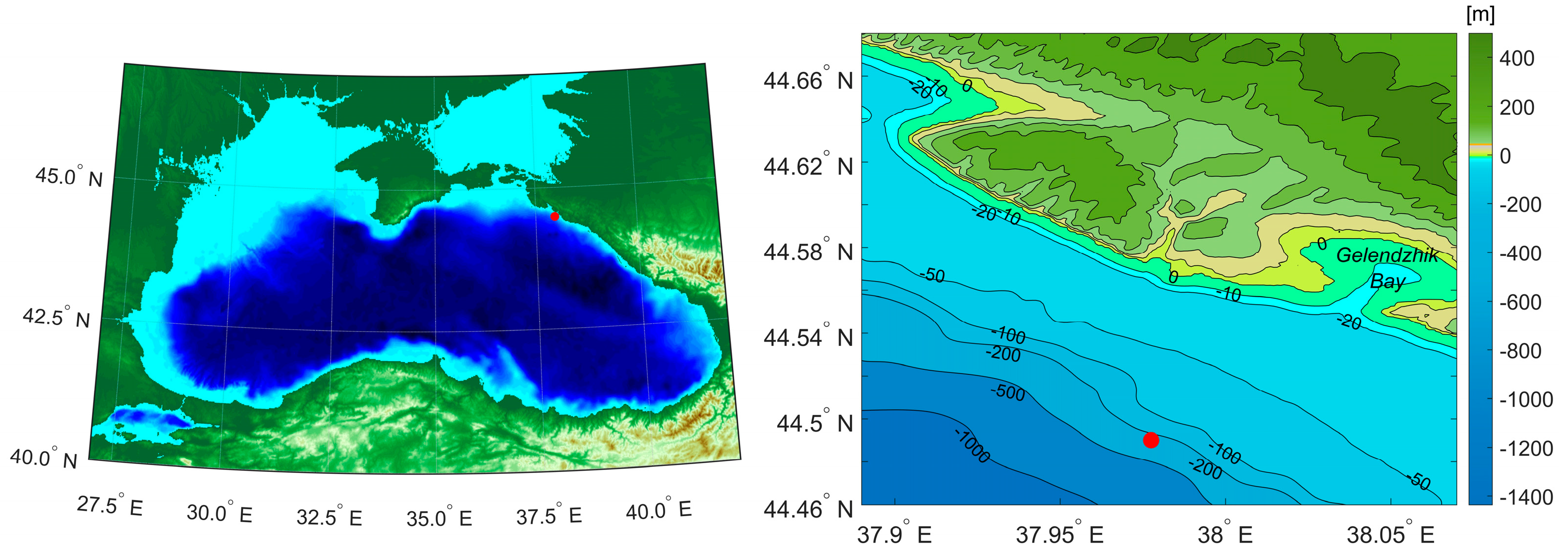
The measurements over the continental slope were carried out using the Aqualog moored profiler equipped with a CTD probe and acoustic Doppler current meter [29]. The mooring was deployed on the 250 m isobath in the upper part of the continental slope near Gelendzhik Bay (Gelendzhik, Russia) (Figure 1). The Aqualog performed automatically ascend/descend cycles no less than every 3 h to obtain at least 16 depth profiles of marine environment measurements per day. The time series of vertical profiles of temperature, salinity, potential density, dissolved oxygen, and current velocity were obtained for the water column from depths of 20–30 m to 200–230 m. During winter and summer conditions, we took the data from 9 January through 6 March 2016 and from 1 June through 27 August 2019, respectively. The measurement data were binned into the depth cells 1 m thick. Note that the profiler was located close to the Rim Current zone on the periphery of the basin-wide cyclonic gyre with NW direction [30].
To gain a comprehensive understanding of the energetics in the water column during observations, we calculated the kinetic energy (KE):
where u and v are the eastward and northward components of current.
Power spectrum analysis was applied to the time series of the sea temperature and potential density data as well as the sea current velocity and KE. Rotary spectral analysis [31,32] was used to obtain the frequency structure of the orbital motions in the horizontal flows. This analysis was carried out for the data obtained through the water column from the sea’s near-surface layer down to the sea’s near-bottom layer. The temporal variability of the zonal (u) and meridional (v) components of current velocity vectors was also analyzed. To eliminate the influence of Doppler distortions and the background current field, the linear trend was first removed. Before conducting spectral analysis, the current data’s time series were filtered using a fourth-order Butterworth bandpass filter for the 0.88–1.11 f band. Note that, unlike spectra, velocity data figures are presented without any filtering. The absence of tides provides us with this opportunity when the inertial manifestations intensify.
After bandpass filtering, the near-inertial kinetic energy (NIKE) was calculated:
where uf and vf are the filtered eastward and northward components of current and ρ is the water density. We used interpolated data with a time resolution of 1 h for the spectral analysis and calculation of KE and NIKE.
3. Results
3.1. Observations of NIWs in Winter Conditions
Figure 2 shows the mean profiles of temperature, salinity, potential density, and the Brunt–Väisäla frequency N for January, February, and March 2016. The process of water cooling was still evident in March, so we considered this period as the final part of the winter season. The cooling process occurred gradually in the upper 120 m layer. Deeper, the cold intermediate layer (CIL) was identified; stratification was almost constant with a temperature close to 8.5 °C. In the 30–50 m layer of the Black Sea, density was primarily controlled by temperature changes due to small variations in salinity. However, in the deeper layer from 50 to 200 m, salinity played a more significant role in vertical stratification than temperature. The salinity in the upper 100 m ranged from 18 to 18.7 PSU, while, in deeper parts, it varied from 18.7 to 21.3 PSU. In January, the most distinct vertical stratification was observed, with a two-layer system and a transition zone at a depth of 110–120 m, which corresponded to the position of the permanent pycnocline. In February and March, the vertical profiles of potential density became smoother and did not show strong separation between layers. In January, the Brunt–Väisäla frequency N reached a maximum of 97 cph at a depth of 118 m. In February and March, N peaked at 84 cph at depths of 119 and 130 m, respectively.
Based on data from the Aqualog profiler between 9 January and 6 March 2016, the upper water layer gradually cooled while the upper mixed layer deepened and the thermocline sharpened (Figure 3). Together with the background deepening of the thermocline, oscillations with a period close to the local inertial one (17.15 h) occurred almost constantly due to the passage of NIWs. The main intensification of inertial movements was observed in January and February. The passage of packets of inertial internal waves was indicated by up and down displacements of the isopycnals. NIWs also appeared in the current velocity data on the continental slope in contrast to the coastal zone where the effects of strong alongshore currents and passing eddies significantly distorted the manifestation of NIWs in currents [25].
The rotary spectra of velocity components from 50 m down to 150 m showed that the anticyclonic rotation slightly prevailed over the cyclonic one with a dominant peak close to the local inertial frequency. Surprisingly, winter observations showed predominance of inertial processes more evident in the frequency spectra of potential density (Figure 4).
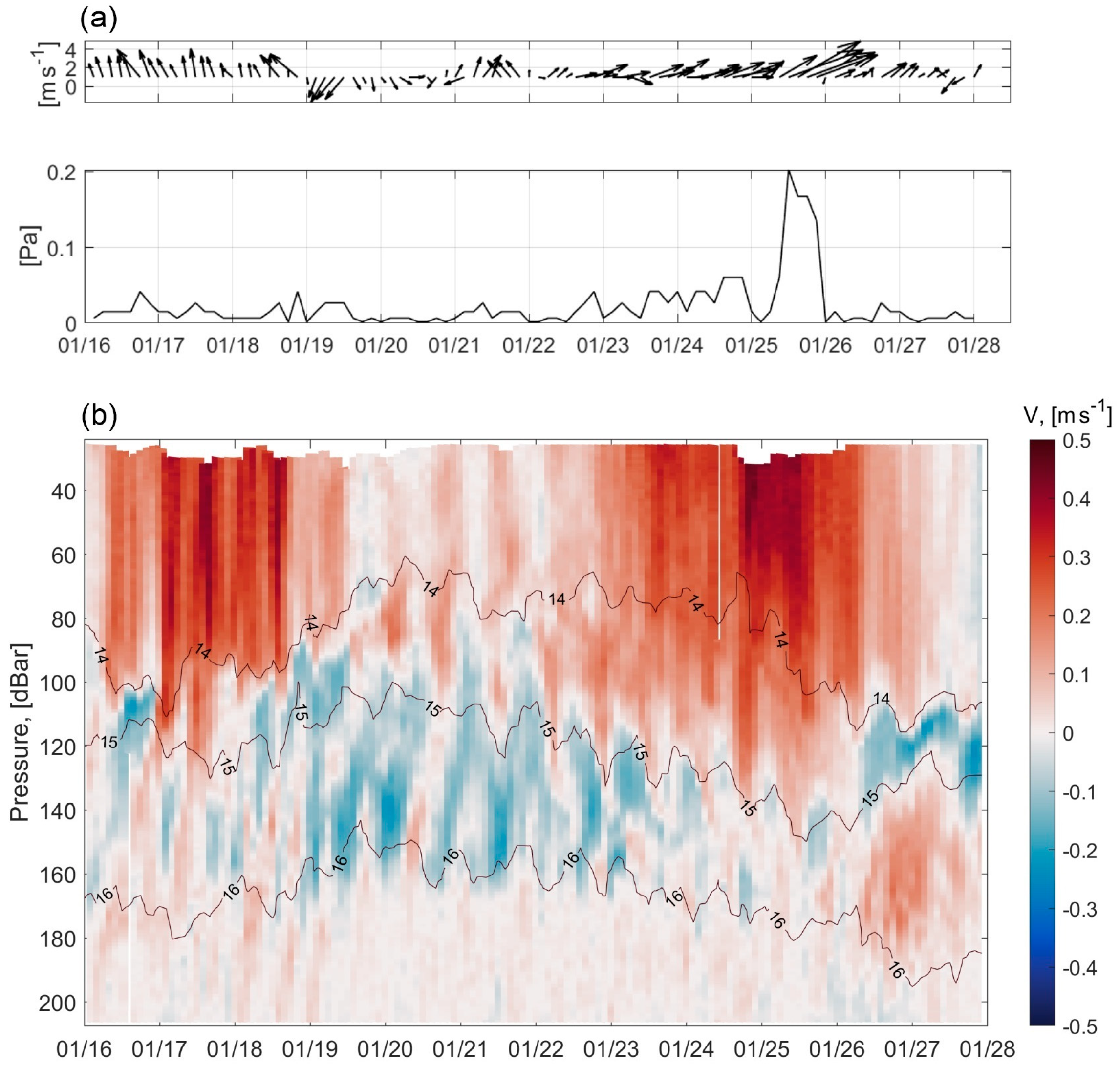
In the winter, the packets of NIWs were observed every month with larger amplitudes from 16 January to 28 January (Figure 5) and from 12 February to 29 February. A packet of intense inertial internal waves was apparent in the current velocity data from 16 January to 28 January. The wave packet travelled within the water lens limited by isopycnals of 14 and 16 kg m−3. Based on observations of displacements of the potential density isolines and velocity measurements, the NIW’s height varied from 30 m up to 100 m. During the passage of the NIW’s crests, the temperature decreased by about 2–3 °C, potential density by 1 kg m−3, and salinity by 1–1.5 PSU. The vertical structure of the near-inertial flow was dominated by a 180° phase difference with one zero-crossing at the depth of the maximum stratification (Figure 5b).
In January, the intensification of NIWs occurred after a change in wind direction during calm weather conditions. The lagged correlation analysis showed no relationship between currents and wind stress in winter (less than 0.4). The maximum correlation of 0.38 with a lag of 2.5 h was observed at a depth of 25 m.
During 16–28 January, there were several periods of KE intensification in the upper layer. The intensifications could be due to meandering of the Rim Current (Figure 6a). This was manifested by an increase in the northern component of the current velocity up to 0.5 m s−1 at the time when KE grew in the 80 m layer. During 19–22 January, the energy maxima during the passage of the NIW packets exceeded 1.5 J m−3. The influence of NIWs was strongest in the layer at 130–150 m depth and extended downward to a depth of 160 m (Figure 6b). On 16 January, NIWs were identified in the layer from 70 m down to 150 m. The maxima variations of NIKE with energy of 1 J m−3 were observed between 100 and 110 m. These NIWs were probably formed by a similar event of northern velocity intensification (not shown).
Two apparent velocity peaks of up to 0.15–0.2 m s−1 were found in the upper mixed layer and below the layer of maximum potential density gradient. The current velocity profiles, in some cases, contained ensembles with a well-defined rotation of the current velocity vector with depth (Figure 7). In the 65–165 m depth layer, regular oscillations indicating a clockwise rotation of the velocity vector with depth were observed in the current velocity data. This suggests that the direction of phase propagation for these waves was upward towards the sea surface, i.e., opposite to the direction of the wave. The vertical phase speed of NIWs varied between 0.1 and 0.24 cm s−1. Several cases of weaker NIWs with downward phase tilt in time were identified between 22 and 24 January.
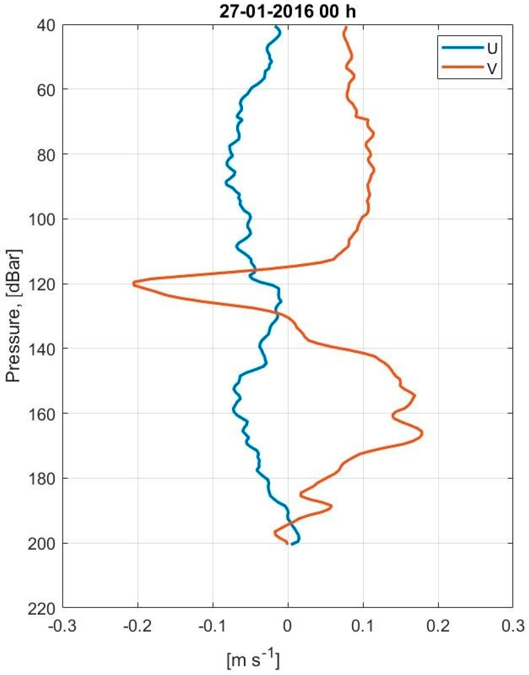
After 26 January, the deepening of the pycnocline was observed and it was found that isopycnals 14 kg m−3 and 16 kg m−3 were out of phase. While the isopycnal surface of 14 kg m−3 was rising, the isopycnal surface of 16 kg m−3 shifted deeper. These changes in vertical stratification caused the appearance of mode-2 NIWs. A velocity peak of 0.1 m s−1 was observed in the upper layer close to 75 m, a second peak of 0.2 m s−1 was revealed at 120 m, and another peak of 0.15 m s−1 was distinguished at 155 m (Figure 8). In the observed wave, therefore, the sign of the horizontal component of the currents changed twice, as predicted by the theory. Five waves were observed by the NIKE distribution. In general, mode-2 NIWs were generated when the pycnocline was at its minimum position throughout the observation period.
3.2. Observations of NIWs in the Summer
Summer observations of 2019 allowed us to observe internal waves in both the seasonal pycnocline and the permanent pycnocline. Figure 9 demonstrates the vertical stratification of temperature, salinity, potential density, and the Brunt–Väisäla frequency N for each month of the summer. In June and July, the first 90 m of the water column experienced seasonal warming. The largest changes were observed in the upper 40 m of the water column, where the Brunt–Väisäla frequency N varied between 60 and 70 cph in June and 150 cph in July. Based on temperature observations, it is evident that the maximum heating of the water column extended down to a depth of 40 m. The 20 °C water was observed at a depth of 40 m at the end of July. As previously stated, the upper part of the Black Sea experienced minimal salinity variations, with density primarily influenced by temperature (Figure 10). The main internal waves occurred in the seasonal pycnocline.
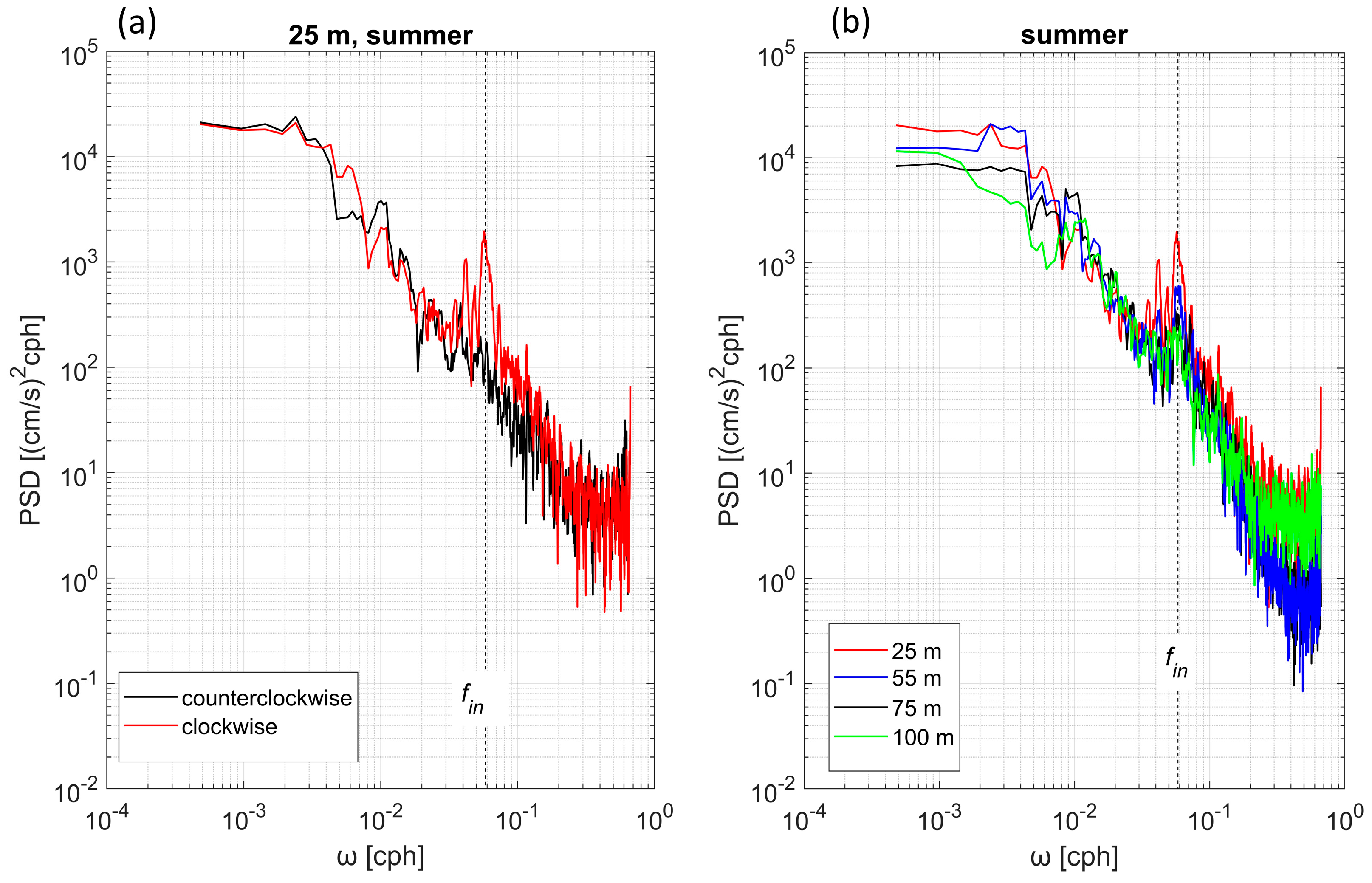
The rotary spectra of velocity components at 25 m depth showed a predominance of the anticyclonic rotation of the current velocity vector (i.e., the current velocity vector rotated clockwise) with a clear-cut peak at a local inertial frequency (Figure 11). A similar analysis was carried out for individual depths, which made it possible to estimate the change in the sea current energy from the near-surface layer down to the near-bottom layer. The near-inertial peak was stronger in the upper part of the water column. The inertial motions were observed down to 55 m depth. Beyond this depth, down to 75 m, the energy level decreased. The level of spectral energy of near-inertial oscillations at 25–55 m was almost five times higher than that at 100–150 m.
Interestingly, the diurnal peak was revealed at 25 m depth. Probably, the diurnal peak was caused by breeze wind circulation. Discussion of this process is beyond the scope of this work.
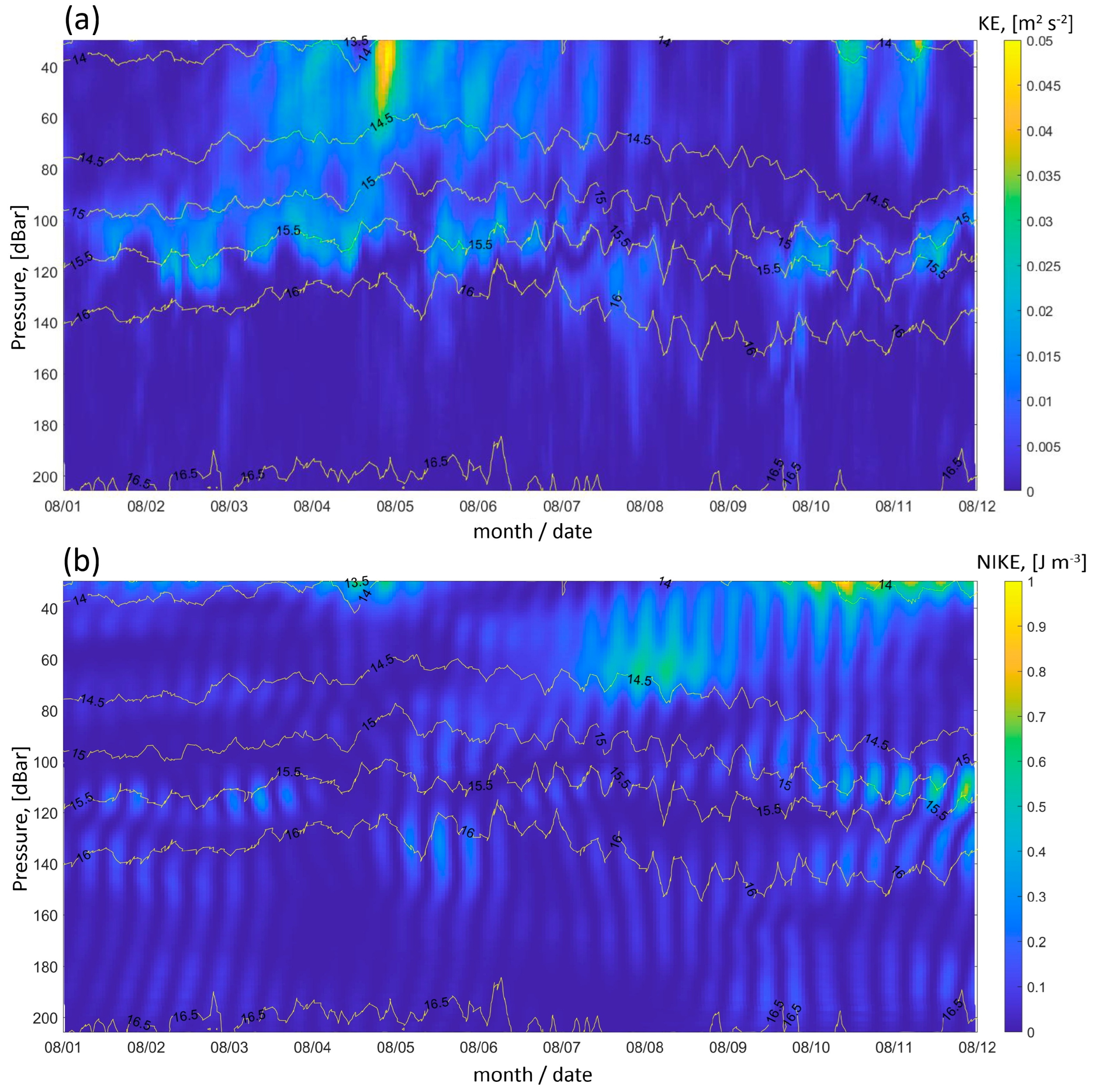
Figure 12 depicts an example of the vertical structure of the eastern component of the currents during the intensification of NIWs from 1 to 11 August. During the inertial wave activity, the main variability occurred in the layer of seasonal pycnocline. The phase difference between the peak upper and lower layer currents was consistent, with a slight phase lead of about 1–2 h in the lower layer. The current meter data showed bursts of near-inertial oscillations with amplitudes as large as 0.1–0.2 m s−1, which were stronger in the upper layer. Additionally, a well-defined clockwise rotation of the current velocity vector with depth was observed from 25 m down to 80–100 m depth. Based on the lagged correlations during NIW episodes between currents at different depths, it was found that all layers have high correlations (~0.7–0.9). In June, the currents at a depth of 25 m lagged behind those at 35 m by about 1 h. In July and August, the lag increased to 24–27 h between 25 m and 45 m. Based on lagged correlations, the vertical phase speed of NIW varied from 0.37 cm s−1 in the upper layer to 0.01 cm s−1 in the deeper part.
The lagged correlation between wind stress and currents at a depth of 25 m exhibited a maximum at 42 h. The circulation of the breeze was evident from the wind direction. Although the wind stress was low during the observation period, the wind stress energy increased on 4–5 August. An upwelling was recorded on 4 August based on temperature measurements. The temperature at a depth of 30 m dropped from 15.5 °C to 9.5 °C. The sea surface temperature decreased by 5–6 °C based on satellite data. Figure 13a shows the increase in KE during the upwelling (note that the scale range is less than in winter). The NIWs observed on 5–8 August may have originated subsequent to the upwelling event. In the time series of NIKE (Figure 13b), the NIWs appeared as a series of slightly inclined swathes of energy maxima of 0.6–0.8 J m−3 with a local maximum at a depth of 60 m. The variations influenced by NIWs extended to a depth of 80 m. More intense inertial motions occurred after three cycles and then decayed slowly.
The pattern of NIKE indicated stronger NIWs in the upper 55 m on 9–11 August. During this event, NIKE reached a maximum of 1.2 J m−3, which was the highest value observed during that period. The first four inertial oscillations occupied the water column down to 80 m depth. Later, the NIWs gradually reduced below 40 m. Strong winds did not occur during this event. The northern component of the currents intensified, probably owing to activity of mesoscale eddies. An increase in KE in the upper 60 m was observed during this period. Also, NIKE increased slightly in the layer of the permanent pycnocline between 100 m and 120 m.
3.3. Comparison of NIWs during Winter and Summer Observations
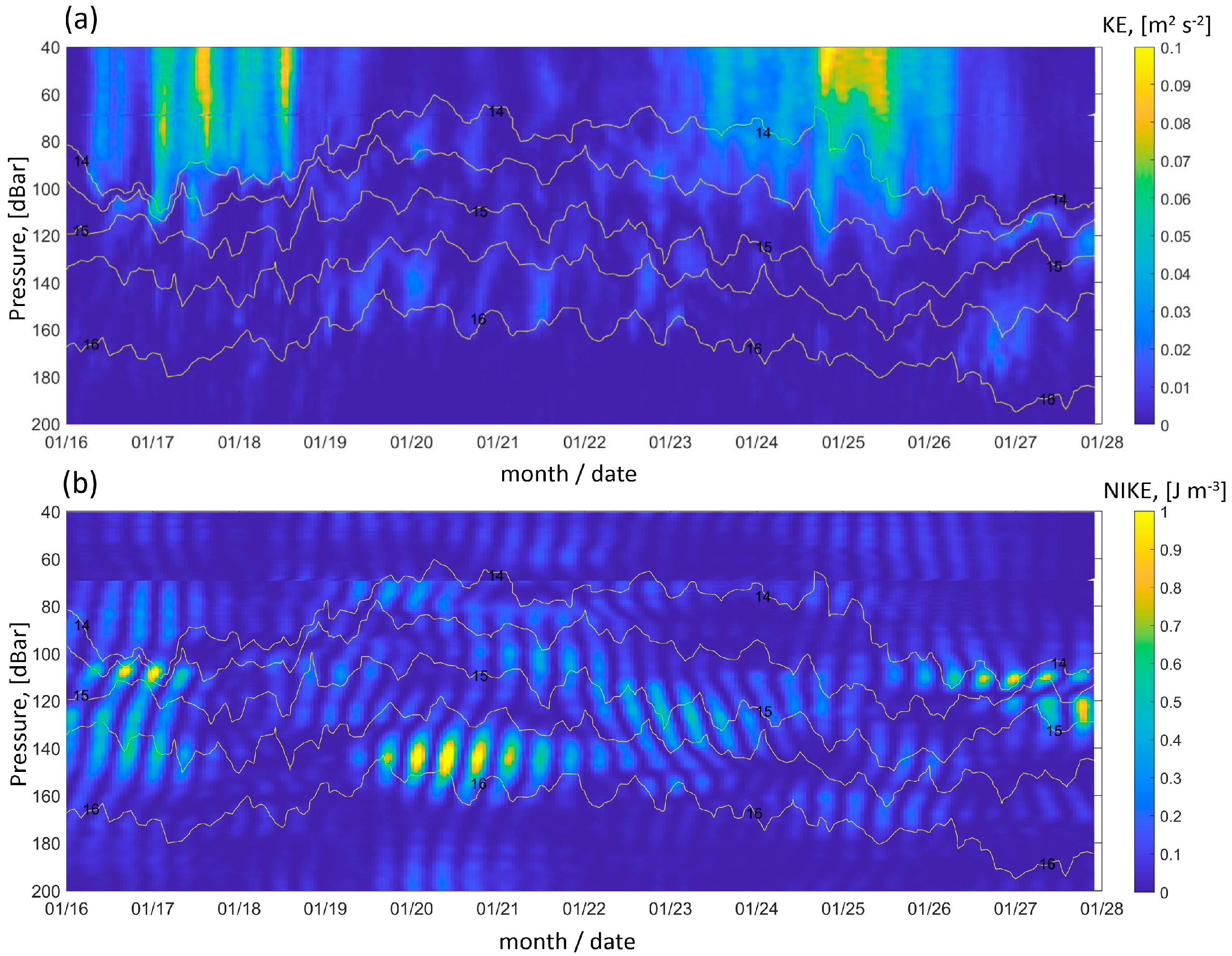
The analysis of seasonal variability of the peaks of the spectra of NIWs revealed their intensification in the upper 60 m layer during the summer season and in the layer of the permanent pycnocline in the winter (Figure 14). The energy level of the frequency spectrum of potential density fluctuations at a depth of 120 m was almost five times higher in winter than in summer. During summer, the energy level at the seasonal pycnocline (30 m) was comparable to that of the permanent pycnocline (120 m) in winter. The minimum energy level was observed at 30 m during winter.
During the winter of 2016, the KE level exhibited maxima ranging from 40 m to 130 m depth in the near-inertial band of 0.88 f–1.1 f (Figure 15a). The peaks of spectrogram of KE over the profiling depth range were shifted to the higher frequency band. In summer, the high KE level was evident down to a depth of 80 m, after which it decreased with depth (Figure 15b). Additionally, there was a slow increase in the layer of the permanent pycnocline between 100 m and 120 m. Note that the energy level during summer was one order of magnitude lower than in winter. The peaks of KE were closer to the local inertial frequency than in winter.
A layer of energy minimum was revealed between 85 m and 95 m during winter and between 80 m and 95 m during summer. Below this layer, there was a subsequent increase in energy within the permanent pycnocline layer, followed by a sharp decrease.
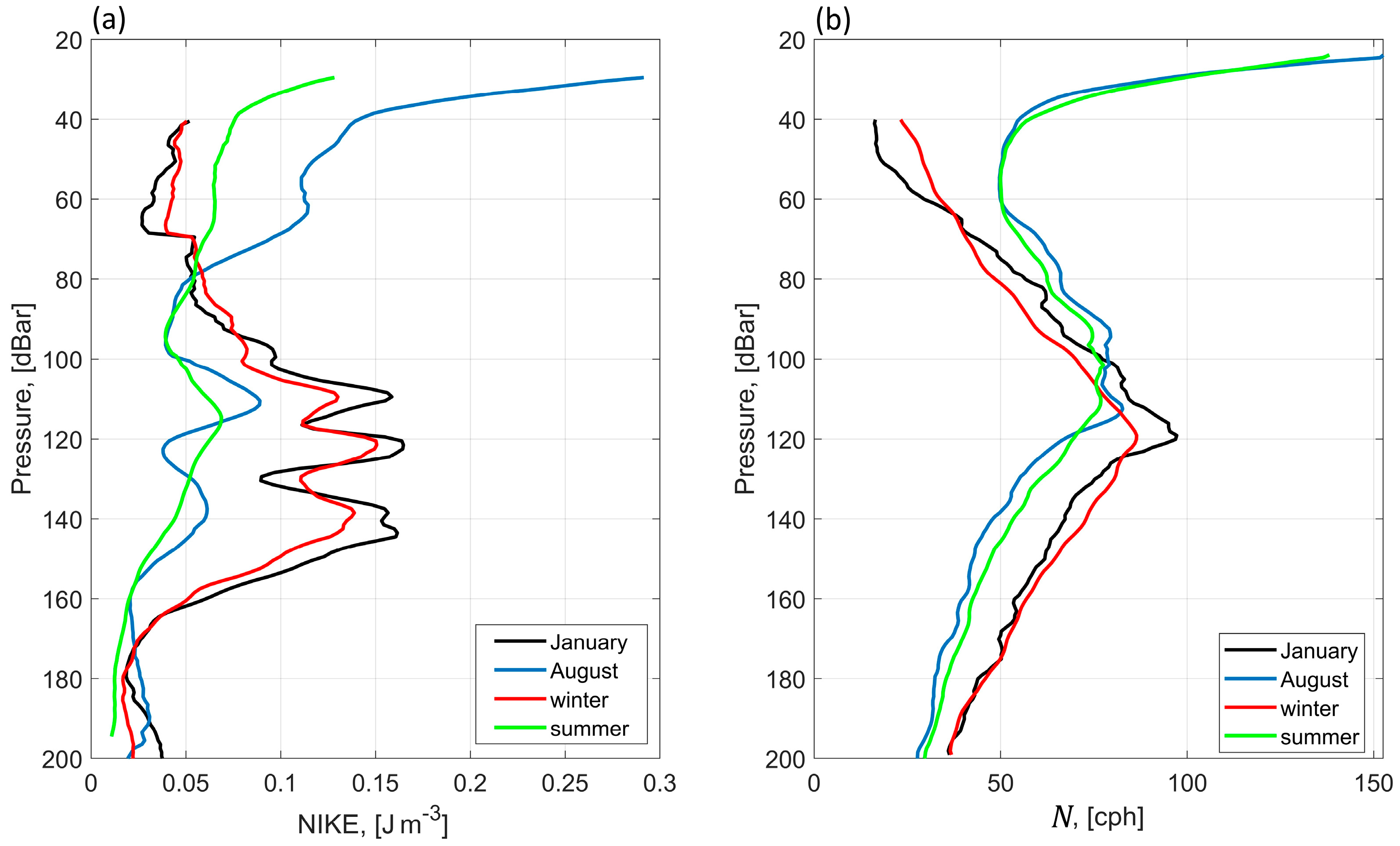
A comparison of the spectrogram of KE over the profiling depth range for the winter with that for the summer suggested that the local stratification had a greater impact on the vertical propagation of NIWs during the observation periods. It seems that the seasonal pycnocline acted as a barrier to NIWs preventing their downward propagation. To clarify this, the mean profiles of NIKE and the Brunt–Väisäla frequency, , were calculated (Figure 16). The amplitude of NIKE showed a close relationship with vertical stratification. The maximum and minimum of energy corresponded to the maximum and minimum of the Brunt–Väisäla frequency.
In winter, the NIKE began to increase at 90 m and reached its maximum (0.15 J m−3) at 120 m.
In summer, the NIKE was larger in the upper 40–60 m. From the mean profiles of NIKE, it was evident that, in summer, the NIKE was mostly intensified in the upper layer up to 0.12 J m−3 but, during strong NIKE events (such as 10–12 August), the energy could penetrate the deeper layer. The NIKE from the mean profiles of August observations had its maximum at 0.28 J m−3 in the 30 m; then, the NIKE decreased sharply below about 80 m.
4. Discussion
The observational data clearly showed the presence of NIWs in the seasonal pycnocline during summer and in the permanent pycnocline during winter in the slope waters in the northeastern part of the Black Sea. The rotary spectra indicated significant peaks in the near-inertial frequencies, with a predominance of anticyclonic rotation in both summer and winter. The velocity data showed that the depth profiles of the eastern and northern velocity components were out of phase, with the northern component leading. The velocity vectors rotated clockwise, with phase lines usually slanted upward in time. This suggested that the direction of phase propagation for identified NIWs was upward towards the sea surface, i.e., opposite to the direction of the wave [33,34]. Previously, a clockwise rotation of the current velocity vector with depth has been observed by lowered ADCP measurements in the northern shelf of the Black Sea [17].
The downward propagation of the NIWs would require their energy sources to be at or near the sea surface. Although it was expected that NIWs would be associated with strong wind events at the study area, they were found to be intense (approximately 0.1–0.2 m s−1) even when the wind stress was weak.
Summer/winter intensification of NIWs in the seasonal/permanent pycnocline indicated that these motions were dependent on thermohaline stratification. The seasonal pycnocline acted as a barrier to NIWs and prevented their downward propagation (see also [35,36]). Basically, KE was much greater in winter than in summer. In winter, the depth–frequency spectra of KE were higher for the layer from 40 m down to 130 m. Noticeably, according to a recent report [37] based on observations, the winter KE increased while the summer KE decreased with depth over the northern shelf of the Black Sea. The increase in the KE in winter could be explained by the propagation of meanders of the Rim Current. The Rim Current was known to intensify in winter and weaken in summer [38,39]. Fluctuations of the baroclinic currents might generate near-inertial oscillations; their energy could be trapped and then propagate downward to the deep layers in regions of negative relative vorticity [40,41]. Previous studies demonstrated the significant influence of mesoscale vorticity on the propagation of NIWs in the ocean [40,42]. Regarding the Black Sea, the Rim Current instability could serve as a source of NIW generation [35]. Our results showed that NIWs were identified when the northern component of the current velocity increased up to 0.5 m s−1 in winter. These intensifications could be associated with the meanders of the Rim Current.
In summer, an increase in NIKE in the upper layer indicated the generation of internal waves by wind. The analyzed data showed an example of observed NIWs that could originate from the upwelling event. In the Black Sea, the generation of internal waves by the upwelling was observed for the high-frequency range [43] and NIWs [44].
Our data showed that NIKE was generally higher in winter than in summer. Previous observations have shown an intensification of NIWs in the central part of the Black Sea during winter [15]. It is noteworthy that manifestations of NIWs were identified in the deep layer at a depth of 1700 m. The present study found that manifestations of NIWs attenuate below 160 m in winter and 80 m in summer. The existence of internal waves at different depths in the central part and over the continental slope of the Black Sea basin can be attributed to the impact of the bottom. Similar to the ocean, the main difference between shelf and deep water NIWs could be explained by the difference in distance between their occurrence and the bottom. The rate of decay due to bottom drag is proportional to the ratio of the bottom mixed layer to the total water depth [45]. In the central part of the Black Sea, measurements were taken in the deep-water area where the bottom drag on NIWs could be considered negligible. However, in the present study, the mooring was deployed at a depth of about 250 m and could be affected by bottom drag. Differences in the vertical scales of NIWs could also be due to the fact that, in slope waters, they can usually interact with background vorticity and mesoscale motions. The Rim Current undergoes meandering behavior, and coastal eddies are frequently observed in the study area [35,46]. However, it should be noted that mesoscale eddy structures also appear in the central part of the Black Sea [47,48]. The NIWs could be trapped by mesoscale structures [1]. These processes are typically intensified near the surface, allowing downward-propagating waves to reach critical layers at depths where the background vorticity decreases.
5. Conclusions
This paper analyzed NIWs on the continental slope of the Black Sea under winter and summer stratification conditions. Field observations were collected using the Aqualog moored profiler, equipped with a CTD probe and an ADCP. NIWs were observed in the near-slope waters within the layer of permanent pycnocline during winter and within the seasonal pycnocline during summer. The clockwise spectrum dominated in the internal wave spectra. The velocity vector rotated clockwise with depth, indicating that the NIWs were propagating downward.
In summer, the vertical structure of the mode-1 baroclinic NIW variability had a zero crossing between 25 m and 100 m, while, in winter, it occurred between 60 m and 160 m. The vertical phase velocity of the NIWs decreased with depth and varied between 0.24 and 0.1 cm s−1 and 0.37 and 0.01 cm s−1 in winter and summer, respectively. During the winter measurements, a case of mode-2 NIWs was identified when the pycnocline deepened and the stratification became sharper.
Significant differences in the seasonal variability of NIWs were observed at different depths in the near-slope region. The amplitude of the NIKE showed a close relationship with vertical stratification, with the maximum and minimum NIKE corresponding to the maximum and minimum Brunt–Väisäla frequency. Near-inertial oscillations were generally more energetic in winter. In summer, the NIKE was stronger in the upper layer of the water column and decreased with depth. In winter, the level of KE was higher between 40 m and 80 m and reached its maximum in the permanent pycnocline layer before dissipating. During the summer season, the KE reached its maximum in the seasonal pycnocline and experienced only a slight increase in the permanent pycnocline. A layer of KE minimum was found between 80 and 95 m in both winter and summer. This is an intriguing feature, considering that these depths do not correspond to the minimum stratification, so further research is needed to clarify the reasons for this energy minimum.
While the study of NIWs in the Black Sea has a long history, our research contributes to the existing knowledge on the subject. We have analyzed long-term measurements of the vertical structure of NIWs under different stratification conditions, which is still rare for Black Sea research. However, to understand the processes of NIW generation and propagation, long-term spatial–time measurements with a high sampling rate are necessary. Therefore, further investigations are needed to obtain a more holistic view of the internal wave field in the Black Sea.
Author Contributions
Conceptualization, E.K.; methodology, E.K. and A.O.; data analysis, E.K.; investigation, A.O. and E.K.; writing—original draft preparation, E.K.; writing—review and editing, E.K. and A.O. All authors have read and agreed to the published version of the manuscript.
Funding
The research was conducted by the assignment of the Ministry of Science and Higher Education of Russian Federation (No. FMWE-2024-0024) and data processing and analysis supported by Russian Science Foundation (project No. 22-77-00055, https://rscf.ru/project/22-77-00055/, accessed on 12 February 2024).
Institutional Review Board Statement
Not applicable.
Informed Consent Statement
Not applicable.
Data Availability Statement
Experimental data are archived at the Ocean Acoustics Laboratory (Shirshov Institute of Oceanology, Russian Academy of Sciences) and available upon request.
Conflicts of Interest
The authors declare no conflicts of interest.
References
- Alford, M.H.; Mackinnon, J.A.; Simmons, H.L.; Nash, J.D. Near-Inertial Internal Gravity Waves in the Ocean. Ann. Rev. Mar. Sci. 2016, 8, 95–123. [Google Scholar] [CrossRef] [PubMed]
- Konyaev, K.V.; Sabinin, K.D. Waves Inside the Ocean; Hydrometeoizdat: St. Petersburg, Russia, 1992. [Google Scholar]
- Pollard, R.T.; Millard, R.C. Comparison between observed and simulated wind-generated inertial oscillations. Deep. Res. 1970, 17, 813–821. [Google Scholar] [CrossRef]
- Garrett, C.; Munk, W. Space-time scales of internal waves: A progress report. J. Geophys. Res. 1975, 80, 291–297. [Google Scholar] [CrossRef]
- Fu, L.-L. Observations and models of inertial waves in the deep ocean. Rev. Geophys. 1981, 19, 141–170. [Google Scholar] [CrossRef]
- MacKinnon, J.A.; Gregg, M.C. Near-inertial waves on the New England shelf: The role of evolving stratification, turbulent dissipation, and bottom drag. J. Phys. Oceanogr. 2005, 35, 2408–2424. [Google Scholar] [CrossRef]
- Alford, M.H.; Whitmont, M. Seasonal and spatial variability of near-inertial kinetic energy from historical moored velocity records. J. Phys. Oceanogr. 2007, 37, 2022–2037. [Google Scholar] [CrossRef]
- Maksimova, E.V. A conceptual view on inertial internal waves in relation to the subinertial flow on the central west Florida shelf. Sci. Rep. 2018, 8, 15952. [Google Scholar] [CrossRef]
- Yang, B.; Hu, P.; Hou, Y. Variation and Episodes of Near-Inertial Internal Waves on the Continental Slope of the Southeastern East China Sea. J. Mar. Sci. Eng. 2021, 9, 916. [Google Scholar] [CrossRef]
- Van der Lee, E.M.; Umlauf, L. Internal wave mixing in the Baltic Sea: Near-inertial waves in the absence of tides. J. Geophys. Res. 2011, 116, C10016. [Google Scholar] [CrossRef]
- Lappe, C.; Umlauf, L. Efficient boundary mixing due to near-inertial waves in a nontidal basin Observations from the Baltic Sea. J. Geophys. Res. Ocean. 2016, 121, 8287–8304. [Google Scholar] [CrossRef]
- Senjyu, T. Observation of near-inertial internal waves in the abyssal Japan Sea. La Mer 2015, 53, 43–51. [Google Scholar]
- Senjyu, T.; Shin, H.-R. Flow intensification due to the superposition of near-inertial internal waves in the abyssal Yamato and Tsushima Basins of the Japan Sea (East Sea). J. Geophys. Res. Ocean. 2021, 126, e2020JC016647. [Google Scholar] [CrossRef]
- Klyuvitkin, A.; Ostrovskii, A.; Lisitzin, A.; Konovalov, S. The Energy Spectrum of the Current Velocity in the Deep Part of the Black Sea. Dokl. Earth Sci. 2019, 488, 1222–1226. [Google Scholar] [CrossRef]
- Khimchenko, E.; Ostrovskii, A.; Klyuvitkin, A.; Piterbarg, L. Seasonal Variability of Near-Inertial Internal Waves in the Deep Central Part of the Black Sea. J. Mar. Sci. Eng. 2022, 10, 557. [Google Scholar] [CrossRef]
- Yampolsky, A.D. Internal waves in the Black Sea as observed at a multi-day anchor station. Proc. IOAS USSR 1960, 39, 111–126. [Google Scholar]
- Morozov, A.N.; Mankovskaya, E.V.; Fedorov, S. Inertial Oscillations in the Northern Part of the Black Sea Based on the Field Observations. Fundam. Prikl. Gidrofiz. 2021, 14, 43–53. [Google Scholar] [CrossRef]
- Medvedev, I.P. Tides in the Black Sea: Observations and numerical modelling. Pure Appl. Geophys. 2018, 175, 1951–1969. [Google Scholar] [CrossRef]
- Garrett, C. What is the “Near-inertial” band and why is it different from the rest of the internal wave spectrum? J. Phys. Oceanogr. 2001, 31, 962–971. [Google Scholar] [CrossRef]
- Le Boyer, A.; Alford, M.H.; Pinkel, R.; Hennon, T.D.; Yang, Y.J.; Ko, D.; Nash, J. Frequency shift of near-inertial waves in the South China sea. J. Phys. Oceanogr. 2020, 50, 1121–1135. [Google Scholar] [CrossRef]
- Mori, K.; Matsuno, T.; Senjyu, T. Seasonal/spatial variations of the near-inertial oscillations in the deep water of the Japan Sea. J. Oceanogr. 2005, 61, 761–773. [Google Scholar] [CrossRef]
- Van Aken, H.M.; van Haren, H.; Maas, L.R.M. The high-resolution vertical structure of internal tides and near inertial waves, measured with an ADCP over the continental slope in the Bay of Biscay. Deep Sea Res. Part I Oceanogr. Res. Pap. 2007, 54, 533–556. [Google Scholar] [CrossRef]
- Serebryany, A.N.; Khimchenko, E.E. Strong Variability of sound velocity in the Black Sea Shelf Zone Caused by Inertial Internal Waves. Acoust. Phys. 2018, 64, 580–589. [Google Scholar] [CrossRef]
- Himchenko, E.E.; Serebrjanyj, A.N. Vnutrennie volny na kavkazskom i krymskom shel’fah Chernogo morja (po letne-osennim nabljudenijam 2011–2016 gg). Okeanol. Issled. 2018, 46, 69–87. [Google Scholar]
- Serebryany, A.; Khimchenko, E.; Zamshin, V.; Popov, O. Features of the Field of Internal Waves on the Abkhazian Shelf of the Black Sea according to Remote Sensing Data and In Situ Measurements. J. Mar. Sci. Eng. 2022, 10, 1342. [Google Scholar] [CrossRef]
- Bondur, V.G.; Sabinin, K.D.; Grebenuk, U.V. Characteristics of Inertial Oscillations Based on the Data of Experimental Measurements of Currents on the Russian Shelf of the Black Sea. Izv. Russ. Acad. Sci. Phys. Atmos. Ocean 2017, 53, 135–142. [Google Scholar] [CrossRef]
- Sabinin, K.D.; Korotaev, G.K. Inercionnye kolebanija v prisutstvii sdvigovogo techenija v okeane. Izv. Ross. Akad. Nauk. Fiz. Atmos. Okeana 2017, 53, 399–405. [Google Scholar]
- Serebryany, A.N.; Khimchenko, E.E. Internal Waves of Mode 2 in the Black Sea. Dokl. Earth Sci. 2019, 488, 1227–1230. [Google Scholar] [CrossRef]
- Ostrovskii, A.G.; Zatsepin, A.G. Intense ventilation of the Black Sea pycnocline due to vertical turbulent exchange in the Rim Current area. Deep Res. Part I Oceanogr. Res. Pap. 2016, 116, 1–13. [Google Scholar] [CrossRef]
- Ostrovskii, A.G.; Zatsepin, A.G.; Solovyev, V.A.; Soloviev, D.M. The short timescale variability of the oxygen inventory in the NE Black Sea slope water. Ocean Sci. 2018, 14, 1567–1579. [Google Scholar] [CrossRef]
- Gonella, J. A rotary-component method for analysing meteorological and oceanographic vector time series. Deep Res. Oceanogr. Abstr. 1972, 19, 833–846. [Google Scholar] [CrossRef]
- Mooers, C.N.K. A technique for the cross spectrum analysis of pairs of complex-valued time series, with emphasis on properties of polarized components and rotational invariants. Deep Res. Oceanogr. Abstr. 1973, 20, 1129–1141. [Google Scholar] [CrossRef]
- Leaman, K.D. The Vertical Propagation of Inertial Waves in the Ocean. Ph.D. Thesis, Massachusetts Institute of Technology, Cambridge, MA, USA, 1975. [Google Scholar]
- Gill, A.E. Atmosphere-Ocean Dynamics; Academic Press: Orlando, FL, USA, 1982. [Google Scholar]
- Blatov, A.S.; Bulgakov, N.P.; Ivanov, V.A.; Kosarev, A.N.; Tujilkin, V.S. Variability of Hydrophysical Fields in the Black Sea; Hydrometeoizdat: St. Petersburg, Russia, 1984. [Google Scholar]
- Ivanov, V.A.; Belokopytov, V.N. Oceanography of the Black Sea; Marine Hydrophysical Institute, NAS of Ukraine: Sevastopol, Ukraine, 2011. [Google Scholar]
- Morozov, A.N.; Mankovskaya, E.V. Modern Studies of Water Dynamics in the North-Western Part of Black Sea from LADCP Measurements. 2021. Available online: http://intercarto.msu.ru/jour/article.php?articleId=947 (accessed on 12 February 2024).
- Zatsepin, A.G.; Kremenetskii, V.V.; Stanichnyi, S.V.; Burdyugov, V.M. Basin Circulation and Mesoscale Dynamics of the Black Sea Affected by Wind. In Modern Dynamics of the Ocean and Atmosphere; Triada: Moscow, Russia, 2010; pp. 347–368. [Google Scholar]
- Ciliberti, S.A.; Jansen, E.; Coppini, G.; Peneva, E.; Azevedo, D.; Causio, S.; Stefanizzi, L.; Creti’, S.; Lecci, R.; Lima, L.; et al. The Black Sea Physics Analysis and Forecasting System within the Framework of the Copernicus Marine Service. J. Mar. Sci. Eng. 2022, 10, 48. [Google Scholar] [CrossRef]
- Kunze, E. Near-inertial wave propagation in geostrophic shear. J. Phys. Oceanogr. 1985, 15, 544–565. [Google Scholar] [CrossRef]
- Mooers, C.N. Several effects of a baroclinic current on the cross-stream propagation of inertial-internal waves. Geophys. Astrophys. Fluid Dyn. 1975, 6, 245–275. [Google Scholar] [CrossRef]
- Jaimes, B.; Shay, L. Near-Inertial Wave Wake of Hurricanes Katrina and Rita over Mesoscale Oceanic Eddies. J. Phys. Oceanogr. 2010, 40, 1320–1337. [Google Scholar] [CrossRef]
- Vlasenko, V.I.; Ivanov, V.A.; Lisichenok, A.D.; Krasin, I.G. Generacija intensivnyh korotkoperiodnyh vnutrennih voln vo frontal’noj zone pribrezhnogo apvel-linga. Morskoj Gidrofiz. Zhurnal. 1997, 3, 3–16. [Google Scholar]
- Vlasenko, V.I.; Ivanov, V.A.; Stashchuk, N.M. Generation of near-inertial motions during upwelling. Phys. Oceanogr. 1996, 36, 43–51. [Google Scholar]
- Gill, A.E. On the Behavior of Internal Waves in the Wakes of Storms. J. Phys. Oceanogr. 1984, 14, 1129–1151. [Google Scholar] [CrossRef]
- Kubryakov, A.A.; Stanichny, S.V.; Zatsepin, A.G.; Kremenetskiy, V.V. Long-term variations of the Black Sea dynamics and their impact on the marine ecosystem. J. Mar. Syst. 2016, 163, 80–94. [Google Scholar] [CrossRef]
- Zatsepin, A.G.; Ginzburg, A.I.; Kostianoy, A.G.; Kremenetskiy, V.V.; Krivosheya, V.G.; Stanichny, S.V.; Poulain, P.M. Observations of Black Sea mesoscale eddies and associated horizontal mixing. J. Geophys. Res. Ocean. 2003, 108, 1–27. [Google Scholar] [CrossRef]
- Kubryakov, A.A.; Stanichny, S.V. Seasonal and interannual variability of the Black Sea eddies and its dependence on characteristics of the large-scale circulation. Deep Res. Part I Oceanogr. Res. Pap. 2015, 97, 80–91. [Google Scholar] [CrossRef]
Figure 1.
The position of the Aqualog profiler (red dot) in the Black Sea and a closer view of the study site. The bathymetric map according to ETOPO1 data (https://doi.org/10.7289/V5C8276M, accessed on 12 February 2024).
Figure 1.
The position of the Aqualog profiler (red dot) in the Black Sea and a closer view of the study site. The bathymetric map according to ETOPO1 data (https://doi.org/10.7289/V5C8276M, accessed on 12 February 2024).

Figure 2.
Vertical profiles of the monthly average temperature, , salinity, S, and potential density, , and the Brunt–Väisäla frequency, , for winter months at the observation site.
Figure 2.
Vertical profiles of the monthly average temperature, , salinity, S, and potential density, , and the Brunt–Väisäla frequency, , for winter months at the observation site.
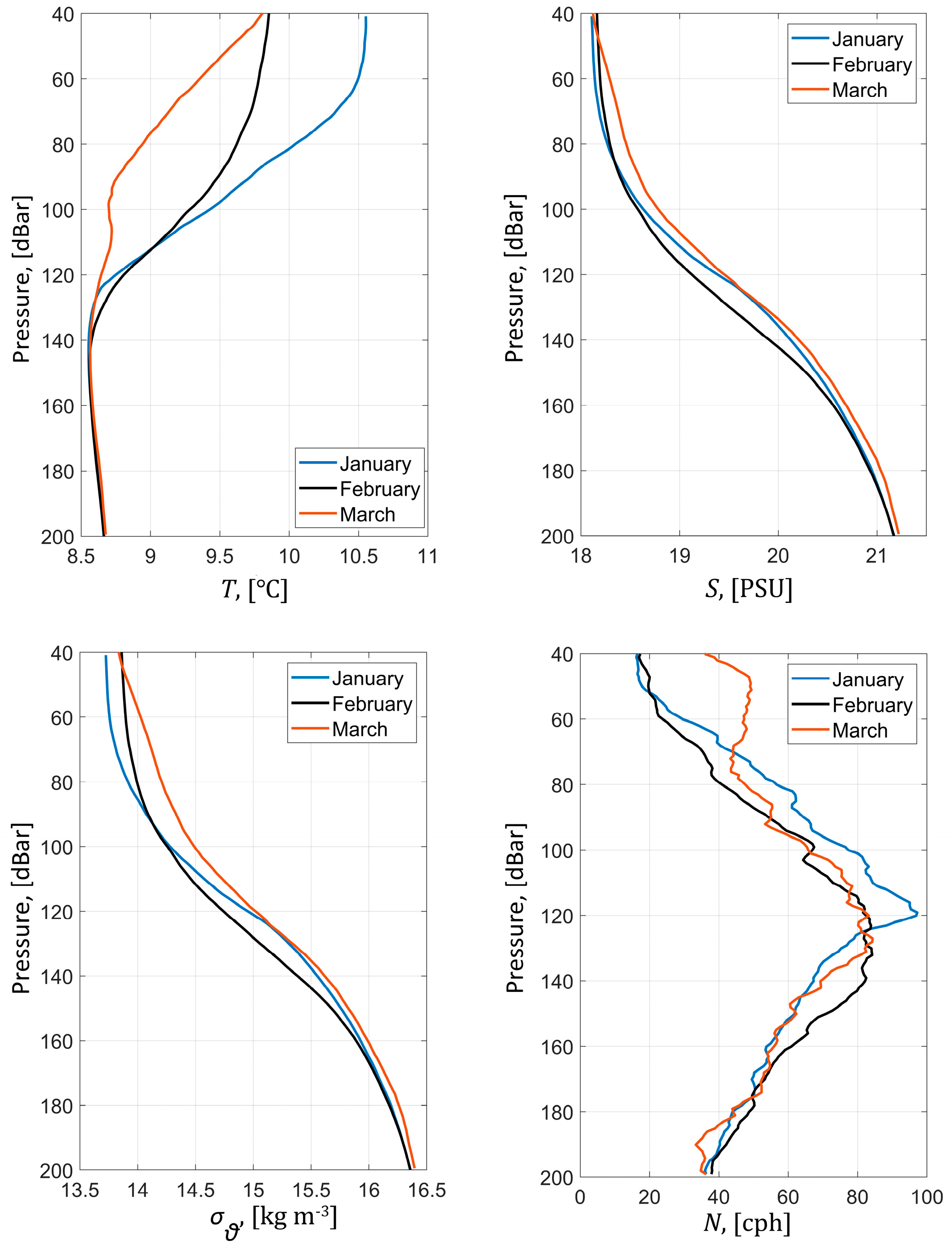
Figure 3.
From top to bottom: the variations in potential density, temperature, and salinity according to the Aqualog profiler data in the depth range from 30 to 220 m between 9 January and 6 March 2016.
Figure 3.
From top to bottom: the variations in potential density, temperature, and salinity according to the Aqualog profiler data in the depth range from 30 to 220 m between 9 January and 6 March 2016.

Figure 4.
The power spectrum of the potential density at 120 m for the entire observation period in 2016. The dash-dotted lines represent the 95% confidence intervals. The black arrow indicates the local inertial frequency.
Figure 4.
The power spectrum of the potential density at 120 m for the entire observation period in 2016. The dash-dotted lines represent the 95% confidence intervals. The black arrow indicates the local inertial frequency.
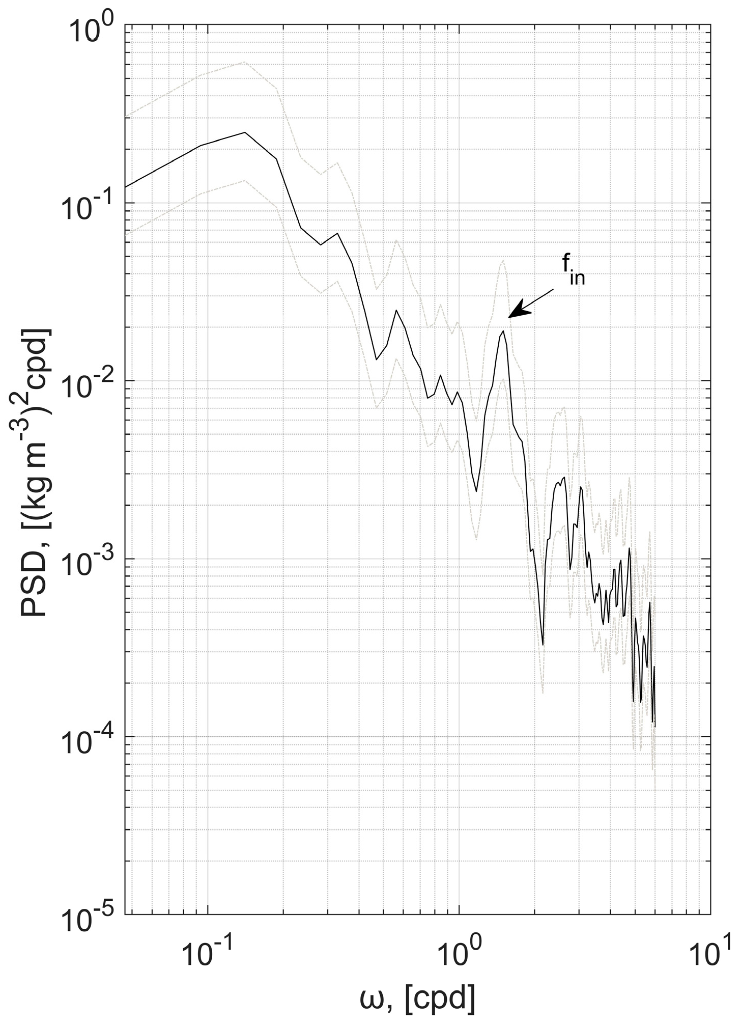
Figure 5.
Time series of wind speed and wind stress (a) and the northern component of the current velocity (b) from 16 to 28 January 2016. The black lines on the graph represent potential density isolines of 14, 15, and 16 kg m−3.
Figure 5.
Time series of wind speed and wind stress (a) and the northern component of the current velocity (b) from 16 to 28 January 2016. The black lines on the graph represent potential density isolines of 14, 15, and 16 kg m−3.

Figure 6.
The time evolution of KE (a) and NIKE (b) during 16–28 January 2016. The isopycnals are shown as solid lines.
Figure 6.
The time evolution of KE (a) and NIKE (b) during 16–28 January 2016. The isopycnals are shown as solid lines.

Figure 7.
The northern component of the current velocity during 20–21 January 2016 (a). The black lines on the graph represent potential density isolines of 14, 15, and 16 kg m−3. (b) Vertical profile of zonal (u) and meridional (v) components at 00:00 20 January 2016.
Figure 7.
The northern component of the current velocity during 20–21 January 2016 (a). The black lines on the graph represent potential density isolines of 14, 15, and 16 kg m−3. (b) Vertical profile of zonal (u) and meridional (v) components at 00:00 20 January 2016.

Figure 8.
Vertical profile of zonal (u) and meridional (v) components at 00:00 27 January 2016.

Figure 9.
The same as Figure 2 but for the summer of 2019.
Figure 9.
The same as Figure 2 but for the summer of 2019.
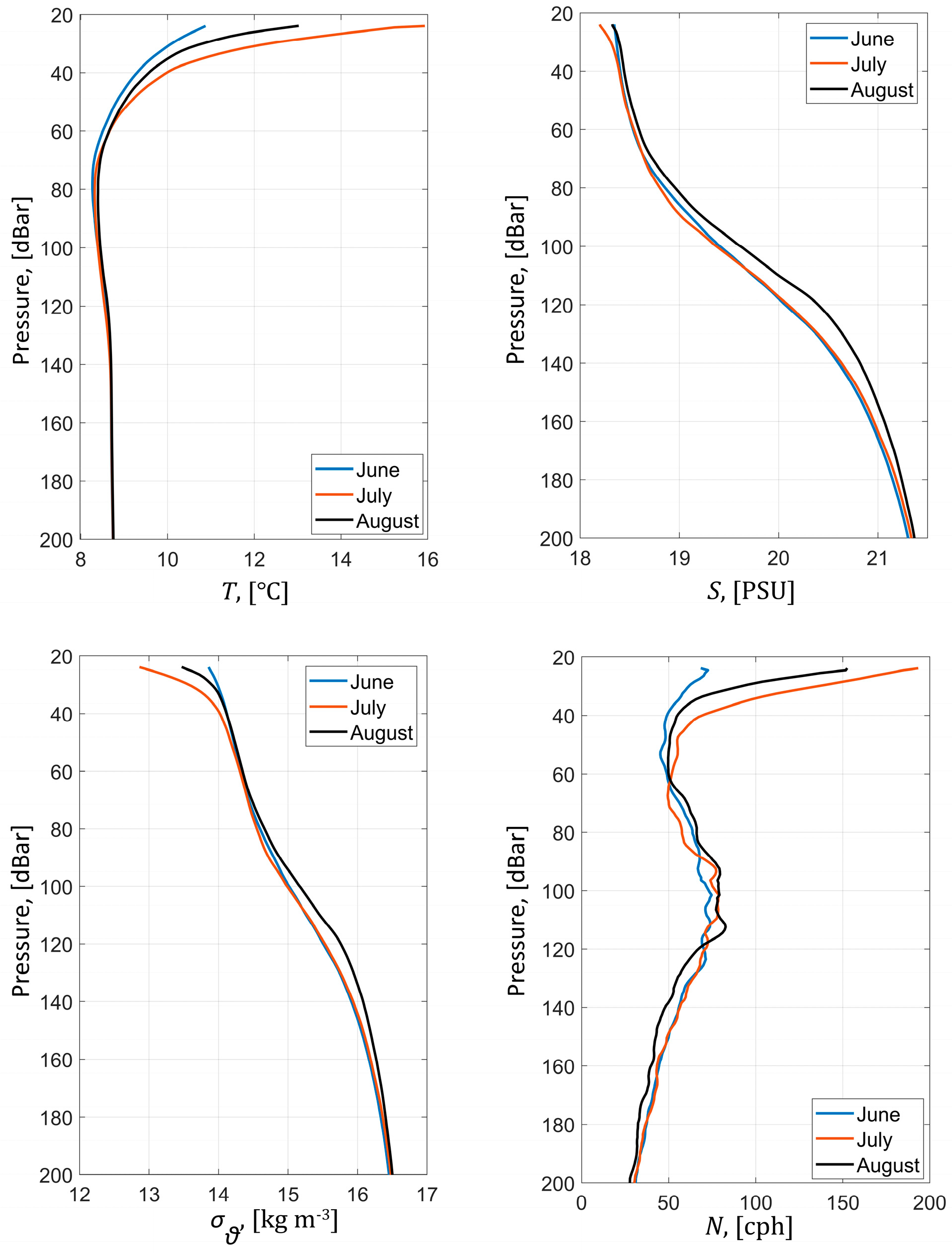
Figure 10.
From top to bottom: the time variations in potential density, temperature, and salinity from 2 June to 26 August 2019, based on the Aqualog profiler data. Note that depth on the vertical axis is shown in the logarithmical scale.
Figure 10.
From top to bottom: the time variations in potential density, temperature, and salinity from 2 June to 26 August 2019, based on the Aqualog profiler data. Note that depth on the vertical axis is shown in the logarithmical scale.
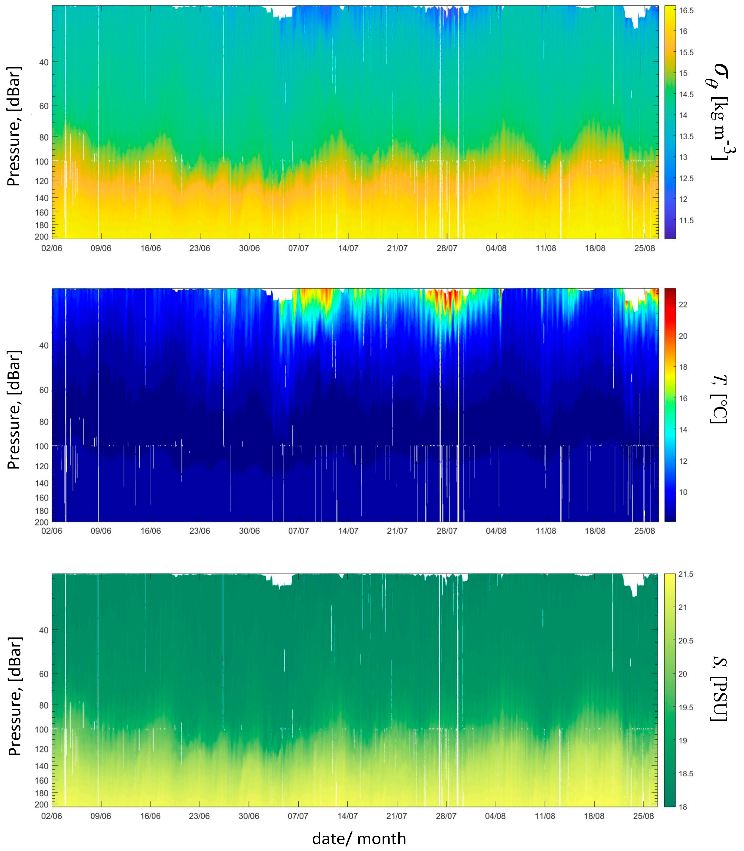
Figure 11.
(a) The rotary spectra of the clockwise and counterclockwise current vector rotation motions at 25 m depth. (b) The rotary spectra of clockwise rotation motion at different depths.
Figure 11.
(a) The rotary spectra of the clockwise and counterclockwise current vector rotation motions at 25 m depth. (b) The rotary spectra of clockwise rotation motion at different depths.

Figure 12.
(a) Time series of wind speed and wind stress; (b) eastern component of currents during 1–11 August 2019.
Figure 12.
(a) Time series of wind speed and wind stress; (b) eastern component of currents during 1–11 August 2019.
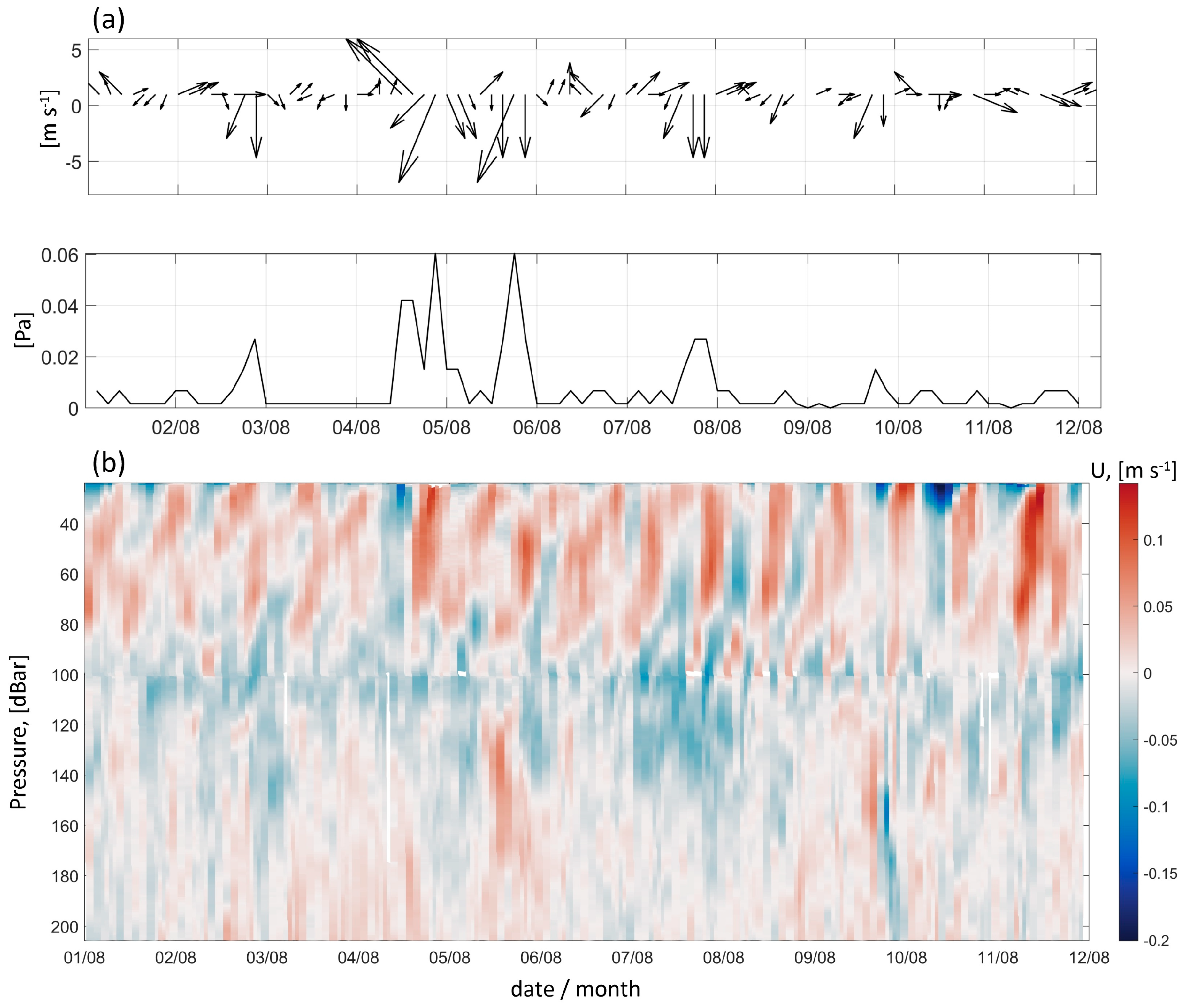
Figure 13.
(a) The time evolution of KE and (b) NIKE during 1–11 August 2019. The isopycnals are shown as solid lines.
Figure 13.
(a) The time evolution of KE and (b) NIKE during 1–11 August 2019. The isopycnals are shown as solid lines.

Figure 14.
The power spectral density of potential density at depths of 30 m and 120 m during winter and summer observations.
Figure 14.
The power spectral density of potential density at depths of 30 m and 120 m during winter and summer observations.

Figure 15.
Spectrogram of KE over the profiling depth range during winter 2016 (a) and summer 2019 (b). A white dotted line indicates the near-inertial frequency. Note that the color bars have different scales.
Figure 15.
Spectrogram of KE over the profiling depth range during winter 2016 (a) and summer 2019 (b). A white dotted line indicates the near-inertial frequency. Note that the color bars have different scales.
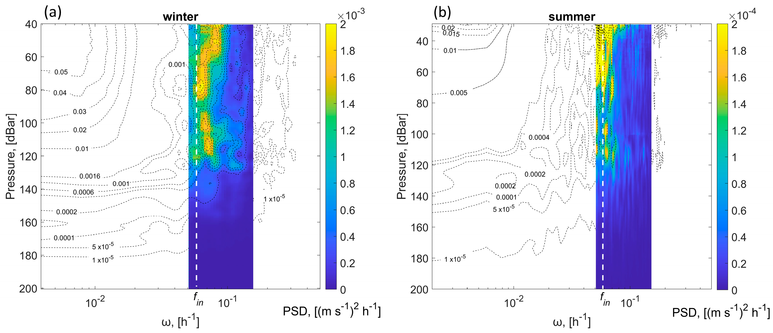
Figure 16.
The mean profiles of NIKE (a) and the Brunt–Väisäla frequency, , (b) for January 2016 and August 2019, winter and summer, during observation periods.
Figure 16.
The mean profiles of NIKE (a) and the Brunt–Väisäla frequency, , (b) for January 2016 and August 2019, winter and summer, during observation periods.
Disclaimer/Publisher’s Note: The statements, opinions and data contained in all publications are solely those of the individual author(s) and contributor(s) and not of MDPI and/or the editor(s). MDPI and/or the editor(s) disclaim responsibility for any injury to people or property resulting from any ideas, methods, instructions or products referred to in the content. |
© 2024 by the authors. Licensee MDPI, Basel, Switzerland. This article is an open access article distributed under the terms and conditions of the Creative Commons Attribution (CC BY) license (https://creativecommons.org/licenses/by/4.0/).
Share and Cite
MDPI and ACS Style
Khimchenko, E.; Ostrovskii, A. Observations of Near-Inertial Internal Waves over the Continental Slope in the Northeastern Black Sea. J. Mar. Sci. Eng. 2024, 12, 507. https://doi.org/10.3390/jmse12030507
AMA Style
Khimchenko E, Ostrovskii A. Observations of Near-Inertial Internal Waves over the Continental Slope in the Northeastern Black Sea. Journal of Marine Science and Engineering. 2024; 12(3):507. https://doi.org/10.3390/jmse12030507
Chicago/Turabian StyleKhimchenko, Elizaveta, and Alexander Ostrovskii. 2024. "Observations of Near-Inertial Internal Waves over the Continental Slope in the Northeastern Black Sea" Journal of Marine Science and Engineering 12, no. 3: 507. https://doi.org/10.3390/jmse12030507
Note that from the first issue of 2016, this journal uses article numbers instead of page numbers. See further details here.