Article

Numerical Simulation of Production Behavior with Different Complex Structure Well Types in Class 1-Type Hydrate Reservoir

1
Guangzhou Marine Geology Survey, China Geological Survey, Ministry of Natural Resources, Guangzhou 511458, China
2
National Engineering Research Center for Gas Hydrate Exploration and Development, Guangzhou 511458, China
*
Authors to whom correspondence should be addressed.
J. Mar. Sci. Eng. 2024, 12(3), 508; https://doi.org/10.3390/jmse12030508
Submission received: 4 February 2024 / Revised: 8 March 2024 / Accepted: 15 March 2024 / Published: 19 March 2024

Abstract

:
Enhancing the production capacity of natural gas hydrates (NGHs) is critical for its commercial development. Complex structure wells may efficiently increase drainage areas while enhancing exploitation efficiency. Based on the field data of China’s first offshore NGH test production, the numerical method was used to analyze the production performance of different complex structure well types by continuous depressurization production for 360 days under the preconditions of fixed effective completion length of 300 m and a pressure difference of 6 MPa. Results indicated that the complex structure well types deployed at the three-phase layer demonstrated superior production performance within 240 days of production; the DLW2 and HW2 well types stood out, with an average gas production rate Qg reaching 43,333 m3/d and a specific production index J of 24.1. After 360 days of production, benefiting from multi-layer combined production, the Cluster vertical well deployed at the multi-layer had the best production performance, with an average Qg of 34,444 m3/d and a J-index of 19.1. The research results provided insights into the complex structure well-type selection strategy for NGH depressurization in this sea area.

Graphical Abstract

1. Introduction

Natural gas hydrates (NGHs) are widely present in permafrost regions and deep-sea sediments. It is estimated that there is approximately 1015–1018 m3 CH4 in the global NGH resources, which is considered to be enough to have the potential to replace fossil fuels [1,2,3,4,5]. The first NGH field test production was completed in 2002 at the Mallik facility in Canada [6]. Recent offshore NGH field test production at Japan’s Nankai Trough and China’s Shenhu Sea area have demonstrated the feasibility and superiority of the depressurization method [7,8,9,10]. However, the offshore field test production capacity remains significantly below the commercialization standard of 50 × 104 m3/d [1]. As a result, improving gas recovery efficiency has become a critical challenge for the industrial exploitation of hydrates. Through the comprehensive analysis of various extraction methods and technologies for NGHs, complex structure well types represented by a horizontal and multilateral well are considered as the primary approaches to increasing NGH productivity [11]. Complex structure wells include all well types except that the traditional vertical well, such as horizontal well, extended reach well, and multilateral well [12].
Therefore, extracting hydrates from complex structured wells has become a research hotspot. For example, Xin X. et al. found that the deployment depth of the lateral branches in a multilateral well is the key factor affecting production capacity [13]. Mao P. et al. evaluated the influence of different parameters related to helical multilateral well on production capacity and believed that it had the potential to achieve commercial development of natural gas hydrates [14]. Ye H. et al. discovered that a directional well and a multilateral well can greatly improve productivity, particularly in a cluster well, which can enhance gas productivity by around 2.2 times compared to a single well [15]. Mahmood M. et al. compared the production capacity of a radial lateral well (RLW) and a horizontal snake well (HSW) in extracting gas hydrates and found that RLW’s productivity is directly related to the number, length, and radius of laterals; two key parameters affect HSW production capacity: one is wellbore length, and the other is radius [16]. Jin G. et al. found that under the same completion length, a multilateral well and a single well produced almost equivalent amounts of gas and water. Interference near branch intersections improves the hydrate dissociation [17]. Ye H. et al. evaluated the impact of different parameter settings on the productivity of different well types, and the results showed that branch parameters have the most significant impact on the productivity of a cluster horizontal well [18]. Hao Y. et al. found that a cluster multilateral well and a fishbone well are the optimal well types for the short- and long-term development of hydrates, respectively [19]. Ye H. et al. found that enlarging the wellbore diameter of a complex structure well can significantly increase production capacity in short-term production [20]. Cao X. et al. found that well interference occurs between lateral branches of a multilateral well, which is unfavorable for gas production and becomes worse as the number of branches increases [21]. Jin G. et al. estimated that 22 sets of multilateral wells each with a completion length of 1000 m are sufficient to achieve commercial development of NGHs in China’s Shenhu Sea area [22]. He J. et al. simulated the productivity of a fishbone well with different lateral branch numbers and found that the production capacity of the six-branch fishbone well was about 59.3% higher than that of the single horizontal well [23].
However, the previous research on complex structure wells mentioned above generally targets 1~4 types of complex structure wells, such as cluster vertical well, cluster horizontal well, herringbone lateral well, and radial lateral well. As of today, both single vertical and single horizontal well have been validated for their technical feasibility through hydrate production testing, and these two types of wells can significantly improve the fault tolerance of the production system. The herringbone lateral well and radial lateral well have not undergone actual application of hydrate production testing, and still face technical challenges in the future. Previous research mainly focuses on the effects of different well deployment or branch lengths, angles, and other parameters of complex structure well on production capacity in the Class 3-type hydrate reservoir. Meanwhile, it is still unclear which complex structure well type has the best production capacity and cost advantage under the different parameter setting in the Class 1-type hydrate reservoir, which consists of an upper hydrate layer and a lower free gas layer (where gas and water can flow freely). The pressure and temperature distribution of the entire reservoir enables the stable existence of hydrates. Therefore, based on the field data of China’s first offshore NGH test production, we take up to eight types of complex structure wells as the research object and use the numerical method to evaluate the production capacity of these well types under the precondition of the total completion length of 300 m and a fixed pressure difference of 6 MPa.

2. Methodology

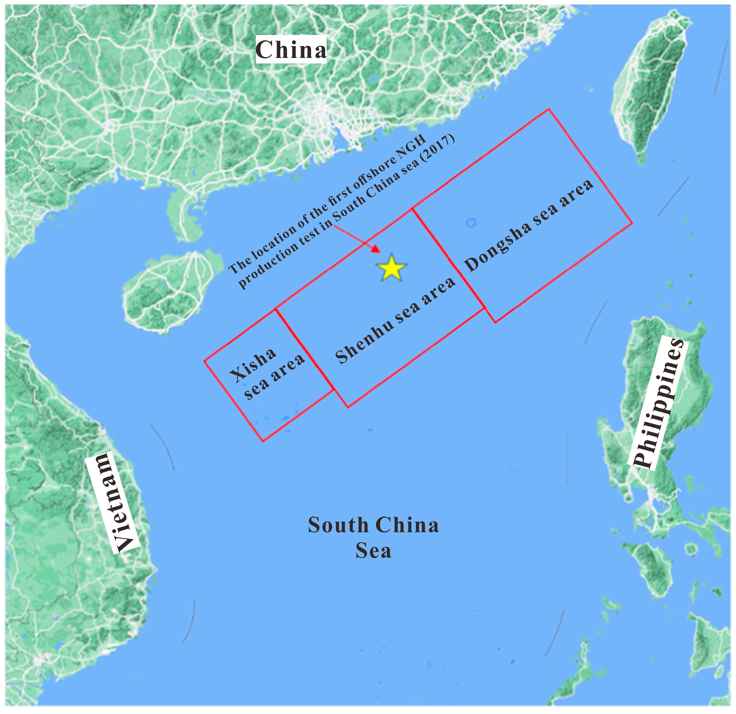
2.1. Geological Background

China’s first offshore NGH test site is located between the Xisha and Dongsha sea areas (Figure 1) [19]. Due to the exceptional geological and engineering conditions, this site is assessed to be the best location for field trials. The water depth at this site is about 1266 m and the seafloor temperature is around 3 °C with a geothermal gradient of 43.653 °C/km [24,25]. The reservoir is mainly composed of three layers: the free gas layer (FGL, 251–278 mbsf, which is composed of low saturation free gas and water), the three-phase layer (TPL, 236–251 mbsf, which contains hydrates, high saturation free gas, and water), and the gas hydrate-bearing layer (GHBL, 201–236 mbsf, which is rich in hydrate and water) [26,27].

2.2. Numerical Simulator

TOUGH+HYDRATE V1.0 is a well-known simulator widely used to predict NGH production [28,29,30]. To overcome the major issue in hydrate modeling, numerous grids are necessary for large-scale simulation [30]. Herein, we used the parallel version of this code and adopted the equilibrium model in this work [31,32]. But it can only simulate up to 50,000 grids, which is insufficient for predicting a large-scale model. Herein, we adopted the parallel version of this code (pT+H v1.0) and the equilibrium model in this work [31,32,33]. Furthermore, the user’s manual for this code has a detailed description of the governing equations [27]. During the simulation process, we assumed that the Darcy’s law is effective in the model and the wellbore is stable. The movement of geological media was neglected. The main governing equations were given as follows [27,34]:
  • Components and phases
Phase(β) = A, G, H, I is aqueous, gas, hydrate, and ice, respectively; Component(κ) = w, m, i, h is water, methane, salt, and hydrate, respectively.
2.
Mass balance
The flow control equation for multi-component fluid mixtures follows mass conservation and is defined as follows:
d d t V n M κ d V = Γ n F κ n d Γ + V n q κ d V
Here, Mκ is the mass accumulation, Fκ is the flux, and qκ is the source/sink ratio.
3.
Energy balance
The heat flow control equation follows energy conservation and is defined as follows:
d d t V n M θ d V = Γ n F θ n d Γ + V n q θ d V
Here, θ is the heat component, Mθ, Fθ, and qθ are the heat accumulation, flux, and source/sink ratio, respectively.

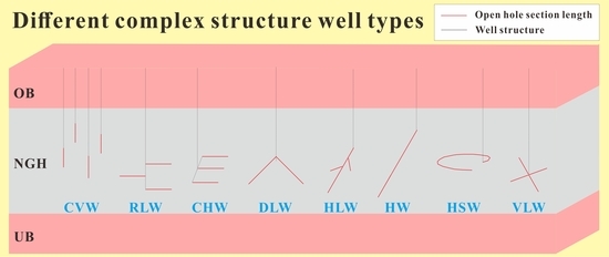
2.3. Model Construction and Well Type Design

The logging curve of SHSC-4 was used to establish the reservoir’s numerical model (Figure 2a), and the domain was 510 × 680 × 117 m in (x, y, z). The boundary layer with 20 m is enough to eliminate the boundary effects [35]. The reservoir can be divided into three layers based on the logging curve. The thicknesses of GHBL, TPL, and FGL were 35, 15, and 27 m, respectively [36]. To evaluate the gas production performance for different complex structure well types, a total of eight well types, including twenty-four simulation cases, were established in this work: (1) Cluster vertical well (CVW): CVW had four vertical wellbores with a wellbore spacing of 180 m, each vertical wellbore was an open hole completion with a length of 75 m and covered GHBL, TPL, and FGL (abbreviated as ML for multi-layer), as shown in Figure 2b. (2) Radial lateral well (RLW): RLW1–3 each had three lateral wellbores with a total open hole completion length of 300 m. RLW1’s three lateral wellbores were located in the middle of the GHBL and TPL, as well as the upper part of the FGL. RLW2’s three lateral wellbores were located at the top, middle, and lower part of the GHBL. RLW3’s three lateral wellbores were located in the middle of the GHBL, as well as the upper and lower parts of the FGL, as shown in Figure 2c. (3) Cluster horizontal well (CHW): CHW1–3 each had three horizontal wells with a total open hole completion length of 300 m. CHW1–3 were located at the middle of GHBL, TPL, and FGL respectively, while CHW4 were located at the ML, as shown in Figure 2d. (4) Direction lateral well (DLW): DLW1–4 each contained 2 lateral wellbores with a total open hole completion length of 300 m; DLW1–4 were located at the GHBL, TPL, GHBL and ML, respectively, as shown in Figure 2e. (5) Herringbone lateral well (HLW): HLW1–3 had one main wellbore and two lateral wellbores each, with a total open hole completion length of 300 m; HLW1–3 were located at GHBL, TPL, and FGL respectively, as shown in Figure 2f. (6) Horizontal well (HW): HW1–3 had an open hole completion with a length of 300 m; HW1–3 were located at the middle of GHBL, TPL, and FGL, respectively, as shown in Figure 2g. (7) Horizontal snake well (HSW): HSW1–3 with a open hole completion length of 300 m and located in the middle of the GHBL, TPL, and FGL, respectively, as shown in Figure 2h. (8) Vertical lateral well (VLW): VLW1–3 had four lateral wellbores with a total open hole completion length of 300 m; VLW1–3 were located at the GHBL, TPL, and FGL, respectively, as shown in Figure 2i. The above simulation cases were divided into four groups, as listed in Table 1.
The discretization was carried out by the following steps to reduce the number of grids and decrease the computational resources: Different well type x-y plane domains were discretized separately and then extruded into 3D discretized grids along the z-axis. To depict the intricate multiphase flow near the wellbore, the minimum grid sizes in the x-, y- and z-axis directions were 2 m, 2 m, and 1 m, respectively. The x-y plane domain of the different well types, CVW, RLW, CHW, DLW, HLW, HW, HSW, and VLW were discretized into 13,923, 2166, 7469, 3040, 5341, 1740, 5478, and 7055 grids, respectively. The total grid was 1,127,763, 175,446, 604,989, 246,240, 432,621, 140,940, 443,718, and 571,455 respectively.

2.4. Initial and Boundary Conditions

The initial conditions of the model can be calculated by the code’s self-balancing function, as shown in Figure 3 [36,37,38,39]. In order to establish the Dirichlet boundary, the top and bottom of the model were set to a fixed temperature and pressure [40]. The wellbore grids were given a fixed pressure difference of 6 MPa and pressure loss along the wellbore was ignored.
The reservoir characteristics (porosity, permeability, saturation) of each sublayer were according to the on-site measured data as follows: (a) The’ porosity values of the three sublayers were 0.35, 0.33 and 0.32; (b) the permeability values of the three sublayers were 2.9, 1.5, and 7.4 mD; (c) the initial gas and hydrate saturations of the GHBL, TPL, and FGL were extracted from the logging curve [9]. It was assumed that the mean porosity of the OB and UB was 0.3 and the permeability was 2.0 mD. Table 2 lists the model’s detailed parameter settings.

2.5. Grid Independence Test

The numerical models established in this work were discretized separately in x-y plane domains, and the total number of grids between these models was different. To verify the errors of these models in predicting gas and water production within an acceptable range, we conducted the grid independence test. First, a vertical well with a completion section length of 70 m was set in the middle of these models, and then the same production pressure difference of 6 MPa was applied for continuous production for 360 days. Figure 4 shows the production results of these models within 360 days. The inconsistency number of grids among different models has almost no impact on the overall gas and water production. Therefore, these models can be used for subsequent comparison production performance of different complex structure well types.

3. Results and Discussion

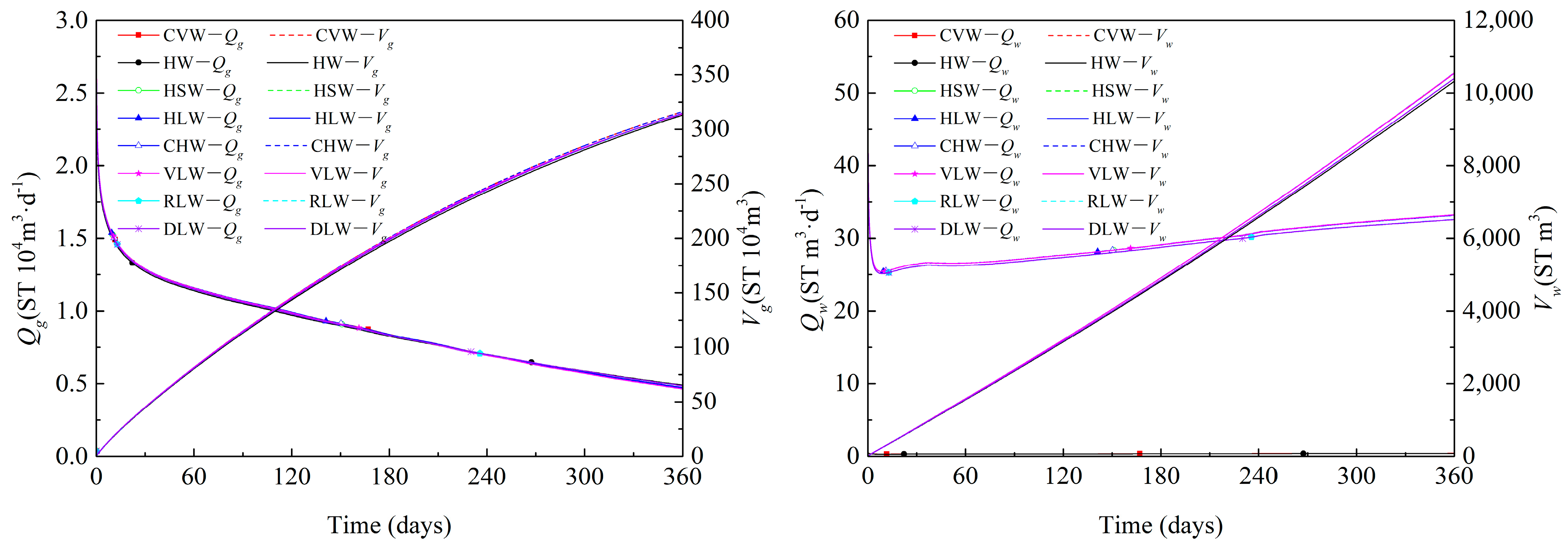
3.1. Well Types Deployed at GHBL

3.1.1. Gas and Water Characteristics

Figure 5a depicts the evolutions of the gas production rate (Qg) and cumulative gas production (Vg) of different well types deployed in the middle of the GHBL within 360 days of production. In the initial stage (within 90 days), the Qg of CHW1, HLW1, HW1, HSW1, and VLW1 were maintained relatively low. The presence of solid hydrates resulted in very low effective permeability of reservoirs. With the decomposition of solid hydrates, the seepage conditions near the wellbore gradually improved. After 90 days of depressurization, the Qg and Vg curves began to show a sudden increase and enter the second stage, which was due to the free gas from the TPL beginning to reach and flow into the wellbores. In the later stage, it was gradually decreasing due to the effects of weak driving force. Unlike the other well types, DLW1 has distinct gas production trends that may likewise be separated into two stages. Qg steadily increases and achieves a high value of 20,597 m3/d in the first stage (within 180 days) and then decreases to 12,966 m3/d by 360 days in the second stage. This is mainly because the lateral branches of DLW covered the entire GHBL and the root ends reached TPL. Due to the weakened of pressure driving force and the sustained Joule–Thomson effect, secondary hydrates were generated at the root ends of its lateral branches. As a result, the average Qg is 16,666 m3/d with a total Vg of 589 × 104 m3 after 360 days of production, which is better than the values of the above well types. The evolution of the water production rate (Qw) corresponds to the gas production behavior as shown in Figure 5b. The gas-to-water ratio Rgw (ST m3 of CH4/ST m3 of water) is an important indicator for assessing gas production efficiency, and a high Rgw means higher recoverability. DLW1 has a higher Rgw of around 170 after 360 days of production, which indicates that it is more adaptable than the other well types during production. Table 3 presents the production capacity of the aforementioned well types.

3.1.2. Characteristics of Reservoir Parameters

As shown in Figure 6a, due to the pressure drop superposition effect, the pressure drop areas between the main wellbore, and lateral branches of DLW1, HLW1, and VLW1 are larger. Similar to the pressure distribution diagram, in the temperature distribution diagram, Figure 6b, under the Joule–Thomson effect and the heat absorption of hydrate decomposition, the temperature near the wellbore of each well type significantly decreases and the low-temperature areas between the main wellbore and lateral branches of DLW1, HLW1 and VLW1 are larger. As shown in Figure 6c,d, after 360 days of production, the saturation of hydrates near the wellbore tends to be almost zero. The released gas accumulates near the wellbore, providing gas for long-term production.

3.2. Well Types Deployed at TPL

3.2.1. Gas and Water Characteristics

Figure 7a shows the evolutions of Qg and Vg of different well types deployed in the middle of TPL within 360 days of production. When the different production well types were deployed in the middle of TPL, the high-saturation free gas of TPL and the hydrate decomposition gas of GHBL could be recovered at the same time, which greatly improved the overall productivity performance. The Qg of all well types reached its peak in the initial stage, but slowly decreased in the later stage due to the weakening of the pressure driving force. As shown in Figure 8c, all well types generated a small amount of secondary hydrates at the root and toe ends of the wellbore after 360 days of production. Among all well types, the DLW2 and HW2 well types had the best productivity performance, with an average Qg of 33,055 m3/d and a total Vg of 1190 × 104 m3 after 360 days of production, and the Rgw of all well types tended to be around 300~400 after 360 days of production. Table 4 presents the production capacity of the aforementioned well types.

3.2.2. Characteristics of Reservoir Parameters

As shown in Figure 8a, the pressure distribution of different well types deployed in the middle of the TPL is similar to that when deployed at the middle of the GHBL, with more obvious and larger areas of pressure drop between the main and lateral branches. It can be seen from Figure 8b that a large amount of gas from TPL is extracted in a short period, which leads to a strong Joule–Thomson effect and the low-temperature areas generated by all well types were significantly larger than those deployed at GHBL. As shown in Figure 8c,d, after 360 days of production, different amounts of secondary hydrates were generated at the root and toe ends of all types of wellbores, and corresponding low gas saturation areas also formed near the wellbores.

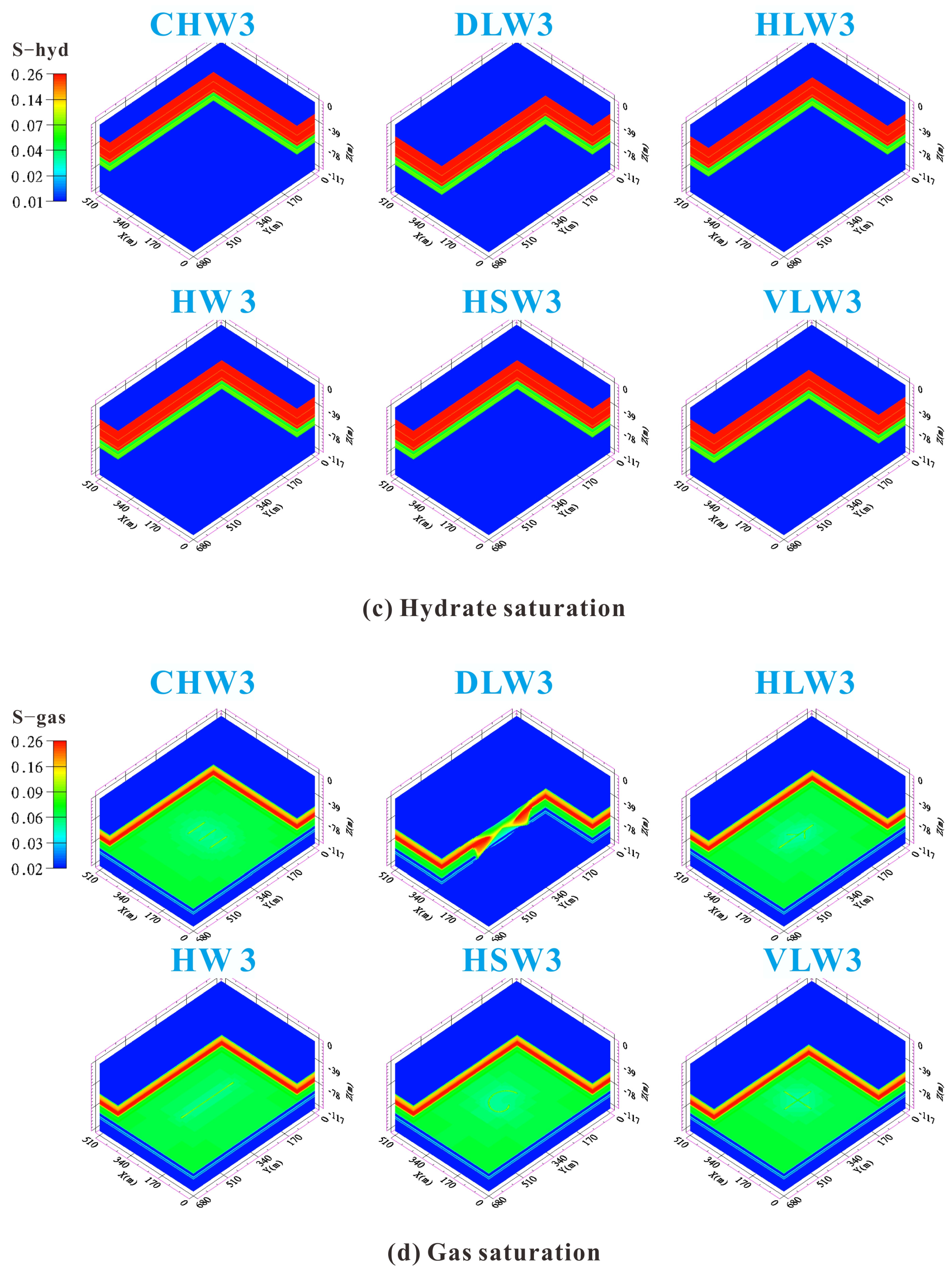
3.3. Well Types Deployed at FGL

3.3.1. Gas and Water Characteristics

Figure 9a depicts the evolutions of Qg and Vg of different well types deployed in the middle of FGL within 360 days of production. The Qg curves of different well types show a sudden increase at 8 days. This is because the high-saturation free gas from TPL begins to reach and flow into the wellbores. Similarly, due to the effects of weak driving force, there is a gradual decrease trend in the later stage. The Qg curves trend of DLW is inconsistent with that of other well types. This is because the lateral branches of DLW cover the entire FGL, and its Qg is the highest among all well types in the initial stage. Among all well types deployed in the middle of the FGL, the HSW3 has the best gas performance, with an average Qg of 24,222 m3/d and a total Vg of 872 × 104 m3 after 360 days of production. Water production behaviors are similar to gas production, as shown in Figure 9b; the Rgw of all well types remains steady around 135~180 after 360 days of production. Table 5 presents the production capacity of the aforementioned well types.

3.3.2. Characteristics of Reservoir Parameters

As shown in Figure 10a, due to the presence of a gas expansion effect in the FGL, the pressure drop cannot be effectively transmitted to a distance; after 360 days of production, the pressure gradient around the DLW’s wellbore is significantly lower than that of other well types. The areas of pressure drop between the main wellbore and lateral branches of other well types are bigger. As for the temperature distribution diagram (Figure 10b), due to the high initial sensible heat in the middle of the FGL, the low-temperature areas are not obvious after 360 days of production for all well types.

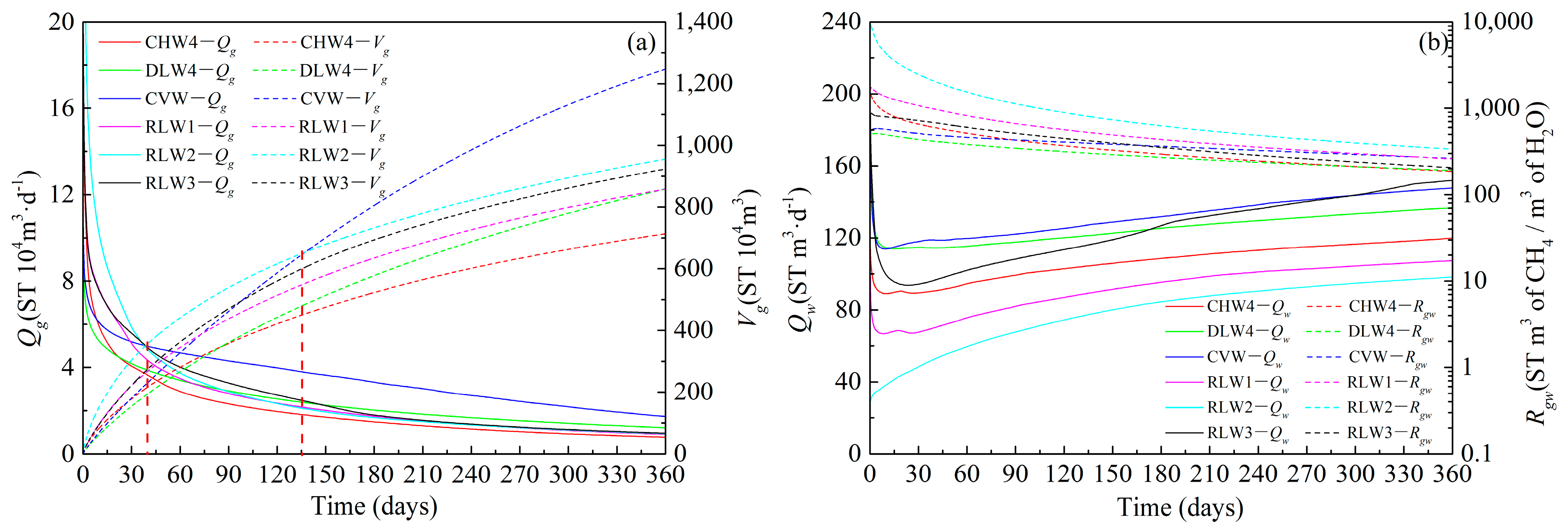
3.4. Well Types Deployed at ML

3.4.1. Gas and Water Characteristics

Figure 11a depicts the evolutions of Qg and Vg of different well types deployed in the middle of ML within 360 days of production. Due to the advantages of multi-layer combined production, the Qg curves peaked early and then gradually declined with the weakening of the driving force in the later stage. After 360 days of production, the CVW well type stood out with a wellbore spacing of 180 m and an average Qg of 34,444 m3/d with a total Vg of 1240 × 104 m3. It is worth noting that starting from 40 days, the Qg of the CVW well type began to surpass that of other well types. After 135 days of production, its Vg also began to surpass that of other well types. The RLW2 well had the highest productivity among the RLW well types because its three lateral branches were located at the upper, middle, and lower parts of the TPL, which means it could effectively recover free gas from the TPL and FGL, as well as hydrate decomposition gas from the GHBL, resulting in the average Qg of 26,527 m3/d with a total Vg of 955 × 104 m3 after 360 days of production. The Rgw of all well types remained steady at around 200~300 after 360 days of production, as shown in Figure 11b. Table 6 presents the production capacity of the aforementioned well types.

3.4.2. Characteristics of Reservoir Parameters

As shown in Figure 12a, it can be observed that the pressure gradient of the lower part of the wellbore structure of all well types was greater than the upper part. Especially for RLW3, the pressure gradient after 360 days of production were significantly lower than other well types. This is mainly because the gas expansion effect in the lower gas-bearing layer limited the pressure propagation. As for the temperature distribution diagram (Figure 12b), the wellbore structures located at the GHBL and TPL layers of all well types formed a noticeable low-temperature area around them. From Figure 12c,d, it can be seen that due to the high initial sensible heat of the FGL, there was no secondary hydrate formation near the wellbore structures located here. Secondary hydrates tend to generate near the wellbore structures located at TPL with high-saturation free gas here, such as the CVW well type where secondary hydrates are most prominent and the gas accumulates near the wellbore.

3.5. Comparisons of Production Performances

In general, the average Qg is the most direct indicator used to evaluate the yield-increasing effect, while relative criterion Rgw is used to evaluate hydrate production efficiency. The yield-increasing mechanism of complex structure wells mainly depends on enlarging the drainage area. However, the increase in production may not be entirely related to the length of completion of the well. Herein, specific index J is recommended as an additional indicator in this section to evaluate production capacity, which is mainly affected by the well type. The following is the definition of the index [10]:
J = Qg/hΔP
h represents the completion length (m), and P represents the pressure difference (MPa). In this work, different complex well types were deployed at the GHBL, TPL, FGL, and ML, respectively. The average Qg and the J index of these well types after 360 days production are shown in Figure 13. Only in terms of production capacity, during the 240-day production period, the production performance of different complex well types with different deployment were as follows: TPL > ML > FGL > GHBL, and the DLW2 and HW2 well types stood out, with an average Qg of 43,333 m3/d and a J-index of 24.1. After 360 days of production, the CVW well type deployed at ML had the best production capacity performance, with an average Qg of 34,444 m3/d and a J-index of 19.1. This is mainly due to the advantage of the multi-layer combined production, as well as the synergistic pressure reduction effect between wellbores. However, it is worth noting that no matter what kind of well type is adopted, one single well production mode cannot meet the commercial development of the offshore NGH. The “well factory” production mode such as a multi-complex well combined with depressurization is the best option for economic exploitation of NGH. Herein, we suggest adopting the CVW as the basic well type for the “well factory” production mode, not only because it has better production performance, but also because the technology threshold and cost involved are relatively low. CVW can improve system redundancy, and any single well can be easily converted into a monitoring or injection well during the production process, which is beneficial for adjusting production plans and requires further research.

4. Conclusions

Based on the field data of China’s NGH test production in the Shenhu Sea area, the numerical method was used to evaluate the production capacity of different complex structure well types by continuous depressurization production for 360 days under the preconditions of fixed effective completion length of 300 m and a pressure difference of 6 MPa. The following results were obtained: during the 240-day production period, the complex structure well deployed at the TPL demonstrated higher production performance, and the DLW2 and HW2 well types stood out with an average Qg of 43,333 m3/d and a J-index of 24.1. After 360 days of production, the CVW deployed at the ML had the best production performance due to the advantage of the multi-layer combined production, as well as the synergistic pressure reduction production effect between wellbores, with an average Qg of 34,444 m3/d and a J-index of 19.1. According to the simulation results, CVW has excellent gas production performance, with the advantages of low technical threshold and cost. More importantly, CVW can improve the fault tolerance of the production system and can easily convert any single well into a monitoring well or injection well. Herein, we suggest adopting CVW as the basic well for the “well factory” production mode, which is worth further research.

Author Contributions

Conceptualization, T.W.; Methodology, T.W.; Software, T.W.; Formal analysis, M.W. and Z.C.; Investigation, M.W. and Z.C.; Resources, L.T.; Data curation, Q.L. and J.Q.; Writing—original draft, T.W.; Writing—review & editing, Z.L.; Visualization, Q.L. and J.Q.; Supervision, Z.L. and J.W.; Project administration, J.W. All authors have read and agreed to the published version of the manuscript.

Funding

This research was funded by the National Key Research and Development Program of China (No. 2021YFB3401405); National Key Research and Development Program of China (No. SQ2023YFC2800361); Guangdong Basic and Applied Basic Research Foundation (No. 2022A1515011902); Guangzhou Science and Technology Program (No. 202206050002); and the Director General’s Scientific Research Fund of Guangzhou Marine Geological Survey, China (No. 2023GMGSJZJJ00027) for financial assistance to this research.

Data Availability Statement

The data presented in this study are available on request from the corresponding author.

Conflicts of Interest

The authors declare that they do not have any commercial or associative interests that represent conflicts of interest in connection with the submitted work.

Nomenclature

Symbols
Lopen hole section length of wellbore (m)
llength of each lateral wellbore or single wellbore (m)
nquantity of lateral wellbore or single wellbore
ttimes (s)
x, y, zcartesian coordinates (m)
Qggas production rates at well (m3/d)
Qwwater production rates at well (m3/d)
Vgcumulative gas production at well (m3/d)
Rgwratio of cumulative gas to cumulative gas(ST m3 of CH4/m3 of H2O)
Jspecific production index
Ttemperature (℃)
Pcapcapillary pressure (Pa)
P0entry pressure of capillary pressure model (Pa)
S*saturation for capillary pressure
SmxAmaximum reference aqueous saturation of capillary
SirAirreducible saturation of aqueous phase
SirGirreducible saturation of gas phase
nApermeability reduction exponent for aqueous phase
nGpermeability reduction exponent for gas phase
λporosity distribution index
kpermeability (m2)
krelative permeability of phase β
φporosity
ρβdensity of phase β
ρRdensity of rock grain (kg/m3)
M κ mass accumulation of component κ, (kg/m3)
F κ mass flux of component κ, kg/(m2·s)
q κ sink/source of component κ, kg/(m3·s)
M θ energy accumulation (J/m3)
F θ energy flux, J/(m2·s)
q θ sink/source of heat, J/(m3·s)
V volume (m3)
Γ surface area (m2)
βphase, β = A, G, H, I is aqueous, gas, hydrate, and ice, respectively
κcomponent, κ = w, m, i, h is water, methane, salt, and hydrate, respectively
Abbreviations
OBoverburden layer
UBunderburden layer
GHBLgas hydrate bearing layer
TPLthree phase layer
FGLfree gas layer
MLmulti-layer
NGHnatural gas hydrate
HWhorizontal well
CVWcluster vertical well
CHWcluster horizontal well
HLWherringbone lateral well
HSWhorizontal snake well
VLWvertical lateral well
RLWradial lateral well
DLWdirection lateral well

References

  1. Sloan, E. Fundamental principles and applications of natural gas hydrates. Nature 2003, 426, 353–359. [Google Scholar] [CrossRef] [PubMed]
  2. Boswell, R. Is gas hydrate energy within reach? Science 2009, 325, 957–958. [Google Scholar] [CrossRef] [PubMed]
  3. Chong, Z.; Yang, S.; Babu, P.; Linga, P.; Li, X. Review of natural gas hydrates as an energy resource: Prospects and challenges. Appl. Energy 2016, 162, 1633–1652. [Google Scholar] [CrossRef]
  4. Boswell, R.; Collett, T.S. Current perspectives on gas hydrate resources. Energy Environ. Sci. 2011, 4, 1206–1215. [Google Scholar] [CrossRef]
  5. Hassanpouryouzband, A.; Joonaki, E.; Farahani, M.; Takeya, S.; Ruppel, C.; Yang, J.; English, N.; Schicks, J.; Edlmann, K.; Mehrabian, H.; et al. Gas hydrates in sustainable chemistry. Chem. Soc. Rev. 2020, 49, 5225–5309. [Google Scholar] [CrossRef]
  6. Moridis, G.J.; Collett, T.S.; Dallimore, S.R.; Satoh, T.; Hancock, S.; Weatherill, B. Numerical studies of gas production from several CH4 hydrate zones at the Mallik site, Mackenzie Delta, Canada. J. Pet. Sci. Eng. 2004, 43, 219–238. [Google Scholar] [CrossRef]
  7. Yamamoto, K.; Terao, Y.; Fujii, T.; Ikawa, T.; Seki, M.; Matsuzawa, M.; Kanno, T. Operational Overview of the First Offshore Production Test of Methane Hydrates in the Eastern Nankai Trough, Offshore Technology Conference; OnePetro: Richardson, TX, USA, 2014. [Google Scholar]
  8. Yamamoto, K.; Wang, X.X.; Tamaki, M.; Suzuki, K. The second offshore production of methane hydrate in the Nankai Trough and gas production behavior from a heterogeneous methane hydrate reservoir. RSC Adv. 2019, 9, 25987–26013. [Google Scholar] [CrossRef] [PubMed]
  9. Li, J.; Ye, J.; Qin, X.; Qiu, H.; Wu, N.; Lu, H.; Xie, W.; Lu, J.; Peng, F.; Xu, Z.; et al. The first offshore natural gas hydrate production test in South China Sea. China Geol. 2018, 1, 5–16. [Google Scholar] [CrossRef]
  10. Ye, J.; Qin, X.; Xie, W.; Lu, H.; Ma, B.; Qiu, H.; Liang, J.; Lu, J.; Kuang, Z.; Lu, C.; et al. The second natural gas hydrate production test in the South China Sea. China Geol. 2020, 3, 197–209. [Google Scholar] [CrossRef]
  11. Wu, N.; Li, Y.; Wan, Y.; Sun, J.; Huang, L.; Mao, P. Prospect of marine natural gas hydrate stimulation theory and technology system. Nat. Gas Ind. B 2021, 40, 173–187. [Google Scholar] [CrossRef]
  12. Gao, D. Discussin on development modes and engineering techniques for deepwater natural gas and its hydrates. Nat. Gas Ind. 2020, 40, 136–143. [Google Scholar]
  13. Xin, X.; Li, S.; Xu, T.; Yuan, Y. Numerical investigation on gas production performance in methane hydrate of multilateral well under depressurization in Krishna-Godavari basin. Geofluids 2021, 2021, 9936872. [Google Scholar] [CrossRef]
  14. Mao, P.; Wan, Y.; Sun, J.; Li, Y.; Hu, G.; Ning, F.; Wu, N. Numerical study of gas production from fine-grained hydrate reservoirs using a multilateral horizontal well system. Appl. Energy 2021, 301, 117450. [Google Scholar] [CrossRef]
  15. Ye, H.; Wu, X.; Li, D. Numerical Simulation of Natural Gas Hydrate Exploitation in Complex Structure Wells: Productivity Improvement Analysis. Mathematics 2021, 9, 2184. [Google Scholar] [CrossRef]
  16. Mahmood, M.; Guo, B. Productivity comparison of radial lateral wells and horizontal snake wells applied to marine gas hydrate reservoir development. Petroleum 2021, 7, 407–413. [Google Scholar] [CrossRef]
  17. Jin, G.; Peng, Y.; Liu, L.; Su, Z.; Liu, J.; Li, T.; Wu, D. Enhancement of gas production from low-permeability hydrate by radially branched horizontal well: Shenhu Area, South China Sea. Energy 2022, 253, 124129. [Google Scholar] [CrossRef]
  18. Ye, H.; Wu, X.; Li, D.; Jiang, Y. Numerical simulation of productivity improvement of natural gas hydrate with various well types: Influence of branch parameters. J. Nat. Gas Sci. Eng. 2022, 103, 104630. [Google Scholar] [CrossRef]
  19. Hao, Y.; Yang, F.; Wang, J.; Fan, M.; Li, S.; Yang, S.; Wang, C.; Xiao, X. Dynamic analysis of exploitation of different types of multilateral wells of a hydrate reservoir in the South China sea. Energy Fuels 2022, 36, 6083–6095. [Google Scholar] [CrossRef]
  20. Ye, H.; Wu, X.; Guo, G.; Huang, Q.; Chen, J.; Li, D. Application of the enlarged wellbore diameter to gas production enhancement from natural gas hydrates by complex structure well in the Shenhu sea area. Energy 2022, 264, 126025. [Google Scholar] [CrossRef]
  21. Cao, X.; Sun, J.; Qin, F.; Ning, F.; Mao, P.; Gu, Y.; Li, Y.; Zhang, H.; Yu, Y.; Wu, N. Numerical analysis on gas production performance by using a multilateral well system at the first offshore hydrate production test site in the Shenhu area. Energy 2023, 270, 126690. [Google Scholar] [CrossRef]
  22. Jin, G.; Su, Z.; Zhai, H.; Feng, C.; Liu, J.; Peng, Y.; Liu, L. Enhancement of gas production from hydrate reservoir using a novel deployment of multilateral horizontal well. Energy 2023, 270, 126867. [Google Scholar] [CrossRef]
  23. He, J. Numerical simulation of a Class I gas hydrate reservoir depressurized by a fishbone well. Processes 2023, 11, 771. [Google Scholar] [CrossRef]
  24. Qin, X.; Lu, J.; Lu, H.; Qiu, H.; Liang, J.; Kang, D.; Zhan, L.; Lu, H.; Kuang, Z. Coexistence of natural gas hydrate, free gas and water in the gas hydrate system in the Shenhu Area, South China Sea. China Geol. 2020, 3, 210–220. [Google Scholar] [CrossRef]
  25. Zhang, W.; Liang, J.; Lu, J.; Wei, J.; Su, P.; Fang, Y.; Guo, Y.; Yang, S.; Zang, G. Accumulation features and mechanisms of high saturation natural gas hydrate in Shenhu area, northern south China sea. Pet. Explor. Dev. 2017, 44, 708–719. [Google Scholar] [CrossRef]
  26. Sun, Y.; Ma, X.; Guo, W.; Jia, R.; Li, B. Numerical simulation of the short- and long-term production behavior of the first offshore gas hydrate production test in the South China Sea. J. Pet. Sci. Eng. 2019, 181, 106196. [Google Scholar] [CrossRef]
  27. Qin, X.; Liang, Q.; Yang, L.; Qiu, H.; Xie, W.; Liang, J.; Lu, J.; Lu, C.; Lu, H.; Ma, B.; et al. The response of temperature and pressure of hydrate reservoirs in the first gas hydrate production test in South China Sea. Appl. Energy 2020, 278, 115649. [Google Scholar] [CrossRef]
  28. Moridis, G.; Kowalsky, M.; Pruess, K. TOUGH+ Hydrate V1.0 User’s Manual; Report LBNL-0149E; Lawrence Berkeley National Laboratory: Berkeley, CA, USA, 2008. [Google Scholar]
  29. Sun, J.; Ning, F.; Lei, H.; Gai, X.; Sánchez, M.; Lu, J.; Li, Y.; Liu, L.; Liu, C.; Wu, N.; et al. Wellbore stability analysis during drilling through marine gas hydrate-bearing sediments in Shenhu area: A case study. J. Pet. Sci. Eng. 2018, 170, 345–367. [Google Scholar] [CrossRef]
  30. Zhu, H.; Xu, T.; Yuan, Y.; Xia, Y.; Xin, X. Numerical investigation of the natural gas hydrate production tests in the Nankai Trough by incorporating sand migration. Appl. Energy 2020, 275, 115384. [Google Scholar] [CrossRef]
  31. Reagan, M.; Moridis, G.; Johnson, J.; Pan, L.; Freeman, C.; Boyle, K.; Keen, N.; Husebo, J. Field-scale simulation of production from oceanic gas hydrate deposits. Transp. Porous Media 2015, 108, 151–169. [Google Scholar] [CrossRef]
  32. Zhang, K.; Moridis, G.; Wu, Y.; Pruess, K. A domain decompositionapproach for large-scale simulations of flow processes in hydrate-bearing geologic media. In Proceedings of the 6th International Conference on Gas Hydrates, ICGH 2008, Vancouver, BC, Canada, 6–10 July 2008. [Google Scholar]
  33. Yin, Z.; Chong, Z.R.; Tan, H.K.; Linga, P. Review of gas hydrate dissociation kinetic models for energy recovery. J. Nat. Gas Sci. Eng. 2016, 35, 1362–1387. [Google Scholar] [CrossRef]
  34. Okwananke, A.; Hassanpouryouzband, A.; Farahani, M.; Yang, J.; Tohidi, B.; Chuvilin, E.; Istomin, V.; Bukhanov, B. Methane recovery from gas hydrate-bearing sediments: An experimental study on the gas permeation characteristics under varying pressure. J. Pet. Sci. Eng. 2019, 180, 435–444. [Google Scholar] [CrossRef]
  35. Yuan, Y.; Xu, T.; Jin, C.; Zhu, H.; Gong, Y.; Wang, F. Multiphase flow and mechanical behaviors induced by gas production from clayey-silt hydrate reservoirs using horizontal well. J. Clean. Prod. 2021, 328, 129578. [Google Scholar] [CrossRef]
  36. Yu, T.; Guan, G.; Wang, D.; Song, Y.; Abudula, A. Numerical investigation on the long-term gas production behavior at the 2017 Shenhu methane hydrate production-site. Appl. Energy 2021, 285, 116466. [Google Scholar] [CrossRef]
  37. Sun, J.; Zhang, L.; Ning, F.; Lei, H.; Liu, T.; Hu, G.; Lu, H.; Lu, J.; Liu, C.; Jiang, G.; et al. Production potential and stability of hydrate-bearing sediments at the site GMGS3-W19 in the South China Sea: A preliminary feasibility study. Mar. Pet. Geol. 2017, 86, 447–473. [Google Scholar] [CrossRef]
  38. Yuan, Y.; Xu, T.; Xin, X.; Xia, Y. Multiphase Flow Behavior of Layered Methane Hydrate Reservoir Induced by Gas Production. Geofluids 2017, 2017, 7851031. [Google Scholar] [CrossRef]
  39. Sun, J.; Ning, F.; Li, S.; Zhang, K.; Liu, T.; Zhang, L.; Jiang, G.; Wu, N. Numerical simulation of gas production from hydrate-bearing sediments in the Shenhu area by depressurising: The effect of burden permeability. J. Unconv. Oil Gas Resour. 2015, 12, 23–33. [Google Scholar] [CrossRef]
  40. Feng, Y.; Chen, L.; Suzuki, A.; Kogawa, T.; Okajima, J.; Komiya, A.; Maruyama, S. Enhancement of gas production from methane hydrate reservoirs by the combination of hydraulic fracturing and depressurization method. Energy Convers. Manag. 2019, 184, 194–204. [Google Scholar] [CrossRef]
  41. Ma, X.; Sun, Y.; Liu, B.; Guo, W.; Jia, R.; Li, B.; Li, S. Numerical study of depressurization and hot water injection for gas hydrate production in China’s first offshore test site. J. Nat. Gas Sci. Eng. 2020, 83, 103530. [Google Scholar] [CrossRef]
Figure 1. SHSC4 well location diagram (adapted from Ref. [19]).
Jmse 12 00508 g001
Figure 2. Model schematic diagram and well type design: (a) Geological model and Logging curve of SHSC-4 well. (b) Schematic diagram of CVW; (c) Schematic diagram of RLW; (d) Schematic diagram of CHW; (e) Schematic diagram of DLW; (f) Schematic diagram of HLW; (g) Schematic diagram of HW; (h) Schematic diagram of HSW; (i) Schematic diagram of VLW.
Jmse 12 00508 g002
Figure 3. Initial conditions of the model.
Jmse 12 00508 g003
Figure 4. Grid independence test.
Jmse 12 00508 g004
Figure 5. Production performances of different well types deployed at the middle of GHBL within 360 days: (a) Gas production rate Qg and cumulative gas production Vg. (b) Water production rate Qw and gas to water ratio Rgw.
Jmse 12 00508 g005
Figure 6. Spatial distribution diagram of physical properties on different well types deployed at the middle of GHBL, and t = 360 days.
Jmse 12 00508 g006aJmse 12 00508 g006b
Figure 7. Production performances of different well types deployed in the middle of TPL within 360 days: (a) Gas production rate Qg and cumulative gas production Vg. (b) Water production rate Qw and gas to water ratio Rgw.
Jmse 12 00508 g007
Figure 8. Spatial distribution diagram of physical properties on different well types deployed in the middle of TPL, and t = 360 days.
Jmse 12 00508 g008aJmse 12 00508 g008b
Figure 9. Production performances of different well types deployed in the middle of FGL within 360 days: (a) Gas production rate Qg and cumulative gas production Vg. (b) Water production rate Qw and gas to water ratio Rgw.
Jmse 12 00508 g009
Figure 10. Spatial distribution diagram of physical properties on different well types deployed in the middle of FGL, and t = 360 days.
Jmse 12 00508 g010aJmse 12 00508 g010b
Figure 11. Production performances of different well types deployed at ML within 360 days: (a) Gas production rate Qg and cumulative gas production Vg. (b) Water production rate Qw and gas to water ratio Rgw.
Jmse 12 00508 g011
Figure 12. Spatial distribution diagram of physical properties on different well types deployed at ML, and t = 360 days.
Jmse 12 00508 g012aJmse 12 00508 g012b
Figure 13. Histogram of J and average Qg for different well types, and t = 120, 240 and 360 days.
Jmse 12 00508 g013
Table 1. The main parameters of simulation cases.
GroupsCaseMain Parameters
L/(m)l/(m)nLocation of Open Hole Section
ACHW13001003GHBL
DLW13001502
HLW1300502
HW1300//
HSW1300//
VLW1300754
BCHW23001003TPL
DLW23001502
HLW2300502
HW2300//
HSW2300//
VLW2300754
CCHW33001003FGL
DLW33001502
HLW3300502
HW3300//
HSW3300//
VLW3300754
DCHW43001003ML
DLW43001502
CVW300754
RLW13001003
RLW23001003
RLW33001003
Note: n is the quantity of lateral wellbore or single wellbore; ML is the abbreviation for multi-layer.
Table 2. Model’s detailed parameter settings.
ParameterValue and Unit
OB and UB’s thickness [9,21,26,41]20 m
GHBL’s thickness [9,21,26,41]35 m
TPL’s thickness [9,21,26,41]15 m
FGL’s thickness [9,21,26,41]27 m
OB and UB’s permeability2.0 mD
GHBL’s permeability [9,21,26,41]2.9 mD
TPL’s permeability [9,21,26,41]1.5 mD
FGL’s permeability [9,21,26,41]7.4 mD
Wellbore radius [9,21,26,41]0.1 m
Salinity [9,21,26,41]3.5%
GHBL and TPL’s hydrate saturation [9,21,26,41]Reference from logging curve (Figure 2a)
FGL’s gas saturation [9,21,26,41]Reference from logging curve (Figure 2a)
OB and UB’s porosity0.30
GHBL’s porosity [9,21,26,41]0.35
TPL’s porosity [9,21,26,41]0.33
FGL’s porosity [9,21,26,41]0.32
Grain density [21,26,41]2600 kg/m3
Geothermal gradient [21,26,41]43.653 °C/km
Grain specific heat [21,26,41]1000 J·kg−1·K−1
Gas composition [21,26,41]100% CH4
Dry thermal conductivity [21,26,41]1.0 W·m−1·K−1
Wet thermal conductivity [21,26,41]3.1 W·m−1·K−1
Capillary pressure model [21,26,41] P c a p = P 0 S * 1 / λ 1 1 λ , S * = S A S i r A S m x A S i r A
Maximum reference aqueous saturation of capillary SmxA [21,26,41]1
Porosity distribution index λ [21,26,41]0.45
Entry pressure P0 [21,26,41]104 Pa
Relative permeability model [21,26,41]KrA = [(SASirA)/(1 − SirA)]nA, KrG = [(SGSirG)/(1 − SirA)]nG
Permeability reduction exponent for aqueous phase nA [21,26,41]3.5
Permeability reduction exponent for gas phase nG [21,26,41]2.5
Irreducible saturation of gas phase SirG [21,26,41]0.03
Irreducible saturation of aqueous phase SirA [21,26,41]0.30
Table 3. Productivity of different well types deployed at GHBL after 360 days of production.
CaseAverage
Qg (104 m3/d)
Vg (104 m3)Compared to the Reference Case
DLW11.64589224.81%
HSW10.91327124.81%
HLW10.88317120.99%
VLW10.83298113.74%
CHW10.77276105.34%
HW1 (ref)0.73262100.00%
Table 4. Productivity of different well types deployed at the TPL after 360 days of production.
CaseAverage
Qg (104 m3/d)
Vg (104 m3)Compared to the Reference Case
DLW23.311190123.96%
HW23.311190123.96%
HSW23.081110115.63%
CHW23.061100114.58%
HLW22.67960100.00%
VLW2 (ref)2.67960100.00%
Table 5. Productivity of different well types deployed at the FGL after 360 days of production.
CaseAverage
Qg (104 m3/d)
Vg (104 m3)Compared to the Reference Case
HSW32.42872118.16%
HW32.34842114.09%
CHW32.25810109.76%
DLW32.19789106.91%
HLW32.12763103.39%
VLW3 (ref)2.05738100.00%
Table 6. Productivity of different well types deployed at the ML after 360 days of production.
CaseAverage
Qg (104 m3/d)
Vg (104 m3)Compared to the Reference Case
CVW3.441240173.91%
RLW22.65955133.94%
RLW32.56923129.45%
RLW12.38857120.20%
DLW42.38858120.34%
CHW4 (ref)1.98713100.00%
Disclaimer/Publisher’s Note: The statements, opinions and data contained in all publications are solely those of the individual author(s) and contributor(s) and not of MDPI and/or the editor(s). MDPI and/or the editor(s) disclaim responsibility for any injury to people or property resulting from any ideas, methods, instructions or products referred to in the content.

