
Net Transport Patterns of Surficial Marine Sediments in the North Aegean Sea, Greece
1
Hellenic Survey of Geology & Mineral Exploration (HSGME), 13677 Acharnae, Greece
2
Department of Geological Sciences, School of Mining and Metallurgical Engineering, National Technical University of Athens, Zografou Campus, 15773 Athens, Greece
*
Author to whom correspondence should be addressed.
J. Mar. Sci. Eng. 2024, 12(3), 512; https://doi.org/10.3390/jmse12030512
Submission received: 8 February 2024
/
Revised: 12 March 2024
/
Accepted: 15 March 2024
/
Published: 20 March 2024
(This article belongs to the Special Issue Recent Advances in Geological Oceanography II)
Abstract
:The spatial distribution of sediments on the seafloor reflects the various dynamic processes involved in the marine realm. To analyze sediment transport patterns in the North Aegean Sea, 323 surficial samples were obtained and studied. The granulometry data revealed a diverse range of grain sizes of surficial sediments, ranging from purely sandy to clay. The predominant size classes were silt and muddy sand, followed by sandy silt and mud. However, there were very few samples that fell within the clay classes. The sorting coefficient ranged from 0.21 to 5.48, while skewness ranged from −1.09 to 1.29. The sediment transport patterns were analyzed based on the grain-size parameters (mean, sorting, and skewness). The results showed the variability of flow parameters involved in sediment distribution. River influx and longshore drift near the shoreline are the most significant factors affecting sediment transport. At the open sea, sediment distribution is mainly controlled by general water circulation patterns, especially by the outflow of low-salinity waters from the Black Sea through the Dardanelles and the Marmara Sea. The heterogeneity of sediment textural parameters across the study area suggests that seafloor sediments are further reworked in areas where water masses are highly energetic. It can be concluded that open sea water circulation controls sediment distribution patterns at the open shelf, while close to the coast, river discharge plays a key role.
1. Introduction
Sediment distribution in the marine realm is the result of various processes described by the general term, sediment dynamics. Various factors are involved in the process of sediment transport and deposition including sediment supply sources, coastal processes (waves, prevailing winds, storm surges, etc.) water depth, seafloor topography, marine water circulation, physical and chemical properties of marine water (salinity, temperature), biogenic alteration, etc. The dynamic conditions of the system result in a continuous reworking of sediments with cycles of remobilization and redeposition. In terms of hydrodynamics, various mechanisms have been proposed. In the shoreline winds, storms and waves [1] can set sediment into a moving state in various ways (collisions between individual sediment grains, and effect of fluid stresses on individual sediment grains), as proposed by Bagnold [2]. Sediment in suspension can remain in motion for long periods due to various processes governed by fluid mechanics laws (diffusion, advection, convection). In the deeper parts of the basin floor, where coastal processes are less intense, gravity currents can also control sediment distribution. These currents can be the result of salinity contrasts, temperature differences, and sediment load differences and are associated with gravity flow deposits [3]. Other factors that affect sediment transport are the biochemical processes that can play a key role in the behavior and textural characteristics of grains. As described by Lee et al. and Cieśla et al. [4,5], the organic matter composed by living organisms can be absorbed by suspended sediments resulting in the stabilization or flocculation of sediments. This affects the grain-size properties of sediment by producing aggregates of fine material.
The aforementioned processes have a direct imprint on the textural parameters of sediments. In this context, various researchers have tried to uncover sediment transport processes by proposing ways to quantitively identify the spatial variations in the grain-size parameters (mean size, sorting, skewness). The first attempts were based in the assumption that mean grain size is reduced in the direction of sediment transport [6] (1972) but this approach was finally assessed as weak. McLaren [7] combined mean size, sorting, and skewness and proposed that in the direction of sediment transport will have a better sorting and a positive skewness while it is possible to become finer or coarser. McLaren and Bowles [8] presented a modified approach of the previous work, concluding that successive deposits in the direction of sediment transport will become either finer, well sorted and more negatively skewed or coarser, or well sorted and more positively skewed. Gao and Collins [9] identified that these are not the only possible cases and proposed a modified model. The model assumes that the trend analyzed has a higher possibility of occurrence in the direction of net transport than in other directions. It identifies the possible net transport paths by comparing two neighboring sampling sites and employing the three most commonly used grain-size parameters (m, s, and Sk) for trend analysis. Through the comparison of grain-size parameters of the two neighboring sampling sites, a dimensionless trend vector is defined, which has a unit length and an orientation that points from the station with the higher sorting coefficient to that with the lower sorting value. The grain-size trend vectors are generated for each sampling station and its neighboring stations, and a single resultant vector is produced after summing the identified trend vectors. The produced vector depicts the trend of sediment transport at the area that has been sampled. A smoothing process is finally applied in order to reduce background noise. This process averages the produced vector of the previous stage, taking into consideration the neighboring sampling sites, and finally provides a residual vector. Net sediment transport vectors methodology have maximized the utilization of grain size parameters and have been used by various researchers to unlock sediment distribution patterns. In this context, in the present study the methodology of sediment transport vectors has been applied in the North Aegean region of the Aegean Sea. The available dataset is part of the Hellenic Survey of Geology & Mineral Exploration (HSGME) of Greece database. The Hellenic Survey of Geology & Mineral Exploration (HSGME) of Greece (the former Institute of Geology and Mineral Exploration—IGME) has to exhibit a long period of activity in the field of marine geological research. The HSGME marine geology geodatabase [10] encompasses up to 25,000 km of bathymetry and seismic profiles, 3500 surface grab samples (from the upper ~15 cm of the seafloor), and 1200 cores (up to 3.5 m long) analyzed at the laboratories of HSGME, with a focus on sedimentology, and specifically, the distribution of grain size and related statistical parameters [11]. Through the interpretation of this data, sediment distribution maps (scale 1:200,000) have been constructed for the Aegean region [12,13,14].
2. Materials and Methods
2.1. Study Area
The North Aegean (Figure 1) is a tectonically complex area dominated by the presence of major structures, such as the North Aegean Trough, as a physical continuation of the North Anatolian Fault [15], as well as by many other active faults; this complexity favoring the accumulation of geological reserves (raw materials, hydrocarbons). Through this active geological framework, the geomorphological features are in a dynamic state, as revealed by various studies [16] depicting the significant modification during the Quaternary. These processes have resulted in a variable configuration of the marine realm consisting of linear and extended peninsulas (e.g., Chalkidiki), isolated gulfs (Thermaikos), and well-preserved continental plateaus incised by canyons and gullies that represent the past subaerial river pathways of fluvial systems like Strymonikos, Nestos [17], and Evros.
Regarding the composition of the sediments accumulating in the basin through the aforementioned fluvial systems (Strymonas, Nestos, and Evros), as expected, the controlling factor lies in the subaerial exposures of Macedonia and Thraki districts geological formations, providing through erosion a variety of materials consisting mainly of post-Alpine sediments, Eocene and Miocene granitoids, Triassic marbles, and Paleozoic gneisses. The various processes involved in sediment transport are imprinted in the variety of grain-size textures identified in the basin floor, where the entire range of grain sizes (gravely sands to clays) have been identified [14,19]. Close to the coastal area, coarser fractions are dominant (gravel and sand), while at the deeper parts, muddy deposits cover the seafloor.
In the western edge of the North Aegean area, corresponding to the Thermaikos Gulf (Figure 1), the geographical features have contributed to the formation of a relatively isolated gulf, protected from external influences. As a result of freshwater influx carrying fine-grained material, there is a prevalence of fine-grained clasts such as silts and clays in the area. Additionally, sandy material in the vicinity of the continental shelf has been identified as relict pre-Holocene deposits through previous research [20,21,22]. The extent of the continental shelf allows for the deposition of most of the material, while only a small fraction travels to the deeper parts of the North Aegean basin. This fraction is transported through the Sporades basin, an elongated basin that represents the western margin of the North Aegean Trough.
The North Aegean continental shelf, located to the east of the Chalkidiki Peninsula, is a relatively flat plateau with limited variations in its morphology. However, the sediment types present in this region vary significantly, with sand fractions exceeding 40% of the analyzed sediment, thus being of particular interest for raw material exploitation, according to sources [13,23,24] (Figure 2). The distribution of sediment in this region is influenced by hydrodynamic conditions, with fine-grained sediments dominating in low-energy areas and significant sand content in other regions. The highest sand content, exceeding 90%, is observed near the Evros River, Samothraki Island, and between the mainland and Thassos Island. Conversely, the Strymonikos and Kavala Gulfs, the deepest areas of the shelf, and the eastward region of the Athos Peninsula are characterized by mud types and fine-grained sediments. The northeastern to southwestern parts of the North Aegean Sea is dominated by fine-grained muddy sediments, the Sporades Basin is mostly covered by silt, while sandy clays are found in the Skyros Basin.
Given the variations in sediment distribution in this region, it is crucial to estimate sediment transport patterns using granulometry data from surficial samples. This is not only important for rare earth element mining but also for the placement of various infrastructures on the seafloor, such as cables and anchored offshore windmills. Therefore, the goal of the present study is to provide a detailed analysis of sediment transport patterns in the North Aegean Sea, enabling better planning and utilization of the region’s resources.
2.2. Sampling Effort and Laboratory Testing
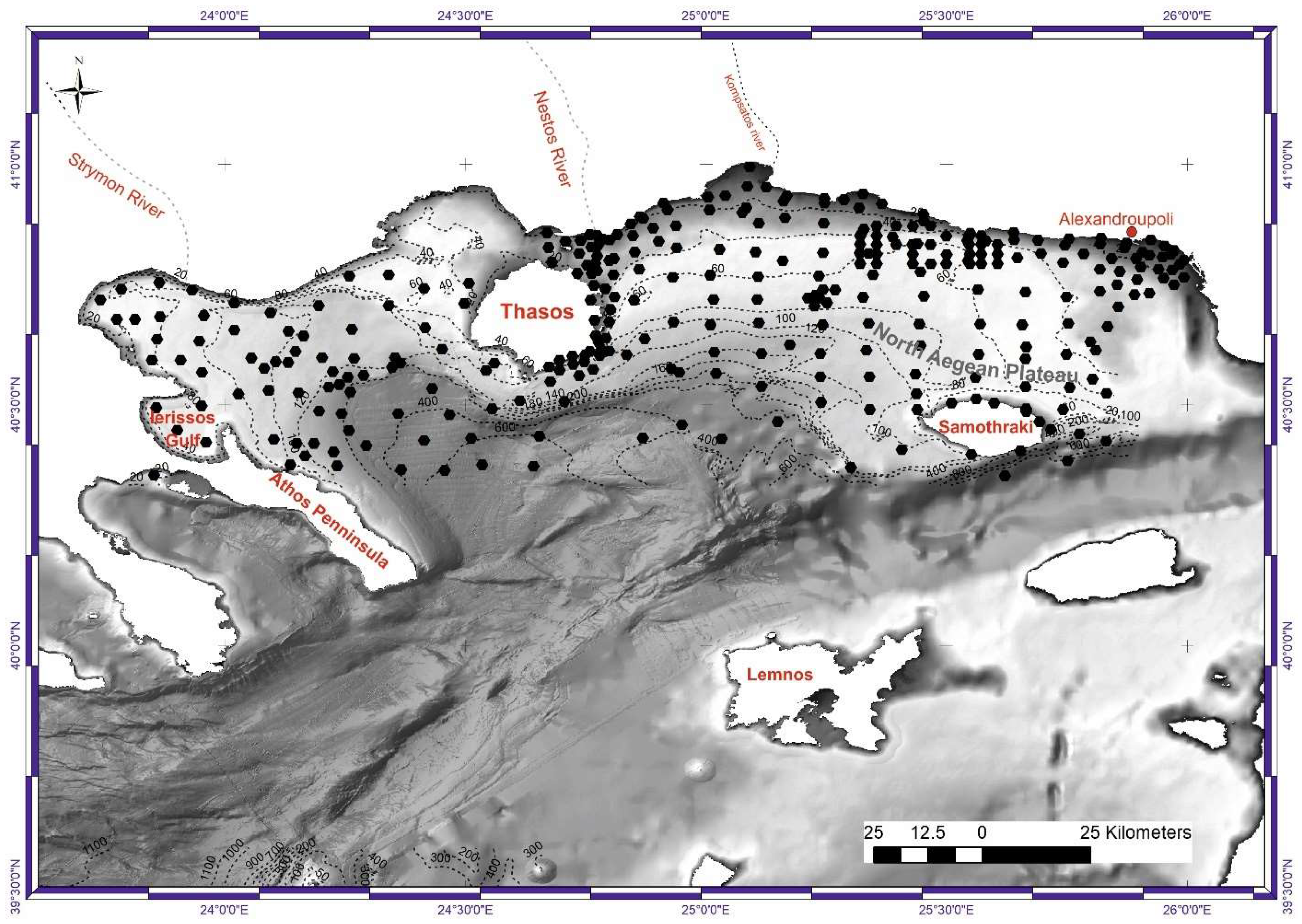
In order to identify sediment distribution patterns, a dataset of 323 point granulometry data, from samples collected during previous field campaigns [14,25], was used. The study area, comprising the northern coastal and open sea of Aegean (Figure 2), covered the region between the Chalkidiki Peninsula and Samothraki Island. The marine environment in this area is variable, ranging from the coastal zone to the shelf areas of Strymonikos and North Aegean plateaus, reaching the shelf break. The sampling depths varied between 0.5 and 693 m. This area is tectonically active, being adjacent to the north Aegean Trough, and exhibits several recent faults and various geomorphological features, such as submerged valleys, slopes, plains, canyons, submarine fans, erosional features, and landslide areas. The aforementioned geomorphological configuration, in combination with marine water circulation, controls sediment transport, reworking, and redeposition and significantly influences the seabed substrate.
Figure 2.
Sampling stations across the study area. Bathymetric contour lines are also shown. The bathymetry hillshade is from the EMODNET database [18].
Figure 2.
Sampling stations across the study area. Bathymetric contour lines are also shown. The bathymetry hillshade is from the EMODNET database [18].
The deposition of coarse-grained sediments is favored in high-energy environments, such as low-relief shallow areas. On the other hand, finer sediments are more likely to accumulate in low-energy habitats where sediments can remain in suspension and reach the most distant coastal areas. The continental shelf’s paleogeographic evolution is shown in the two well-defined paleo-riverbeds of Strymon and Nestos, as identified by detailed bathymetry and seismic profiling studies [17,26]. The onshore geology mainly consists of post-Alpine sediments, Eocene and Miocene granitoids, Triassic marbles, and Paleozoic gneisses [27], whose erosion products are transported offshore via the Strymon River in the NW and a few streams elsewhere, controlling the sediment supply. The grain-size data used for this paper (323 data points) are stored in the Marine Geology Database of HSGME and include data collected from several expeditions carried out between 1979 and 2015 for national mapping and other research projects [10]. The sampling strategy followed a grid based on regular spacing, bathymetry, and acoustic data. The sampling effort varied from a few hundred meters in the shallower part to several kilometers in the deep (Figure 2), with an average of 14.25 points per 100 km2, guided by expert knowledge according to area complexity. The collection of physical samples (grab samples) followed the HSGME Marine Geology Laboratory protocol, and all samples were analyzed in the laboratory according to international protocols [28]. The textural parameters (mean grain size, sorting, and asymmetry) were calculated using the graphical method of Folk and Ward [29]. The results of the textural analysis (mean size, sorting, and skewness) were then used to construct a two-dimensional sediment transport model that reflects sediment transport pathways [7,8]. Net sediment transport patterns were calculated using Gao’s and Collins’ [9,30] grain-size trend analysis. Similar studies from various aquatic realms address the applicability of grain-size trend analysis [31,32,33,34]. This study utilized a two-dimensional model developed by [30] to calculate grain-size trends. The model assumes that the trend analyzed has a higher possibility of occurrence in the direction of net transport than in other directions. It identifies the possible net transport paths by comparing two neighboring sampling sites and employing the three most commonly used grain-size parameters (m, s, and Sk) for trend analysis. The comparison of grain-size parameters of the two neighboring sampling sites, a dimensionless trend vector is defined, which has a unit length and an orientation that points from the station with the higher sorting coefficient to that with the lower sorting value. The grain-size trend vectors are generated for each sampling station and its neighboring stations, and a single resultant vector is produced after summing the identified trend vectors. The produced vector depicts the trend of sediment transport at the area that has been sampled. A smoothing process is finally applied in order to reduce background noise. This process averages the produced vector of the previous stage taking into consideration and the neighboring sampling sites and finally provides a residual vector. The transport vector maps were produced using MATLAB’s GSTA model [35], designed based on Gao’s FORTRAN program [36]. As input parameters were set the mean size, sorting, and skewness of the 323 samples as presented in Table A1 of the Appendix A. The scaling factor A, considering that the used projection is UTM 34N, was set to 1 [36] and the characteristic distance DC was set to 16,000 m.
3. Results
3.1. Grain Size Analyses
The surface sediments were analyzed and classified using the Folk classification method (Figure 3) [11]. The classification results were then plotted on a ternary diagram. The spatial distribution of the sediment classes was estimated using the methodology developed by [14]. Most samples lacked gravel components and were thus plotted onto a Sand/Silt/Clay ternary diagram.
As shown in Figure 4, the eastern part of this study area has a more dominant sand component, reaching up to 80%. This is due to residual sands previously identified in the area during scientific expeditions by HSGME. Increased sand percentages also occur northwest of Thasos Island and in patches near the Athos Peninsula coastline. At depths below 120 m, the sand component decreases rapidly, consisting mainly of benthic and planktonic calcareous skeletal debris. The silt component accumulates in a semicircular depression extending from the east margin of Athos Peninsula to the southwest outer shelf of Thasos Island. A similar trend, with slightly decreased silt component percentages, characterizes the area between the Thasos and Samothraki islands. Silt is less than 30–40% in the rest of the study area, while in sand-dominated areas, it does not exceed values above 20%. The clay fraction is generally underrepresented in the study area, not exceeding 30–40%; however, in the vicinity of river mouths such as Strymon, Nestos, and Kompsatos, the clay fraction reaches up to 50%.
3.2. Grain Size Parameters
The spatial distribution of the mean diameter of the surface sediments reveals two trends (Figure 5a). Firstly, there is a trend of fining towards the deeper parts of the study area, with a slight variation close to Stymonikos Gulf. Secondly, there is a trend of coarsening towards the northeast. The mean diameter of the surface sediments ranges from −0.85φ to 8.31φ.
In the north of Samothraki Island, the mean diameters range from 2 to 4φ, corresponding to medium to very-fine sand, respectively. Finer sediments are found in the perimeter of this area, with mean size values ranging from 4φ to 8φ (very fine sands and silts). As expected, in the depression between Athos and Samothraki, which is generally marked by the 120 to 140-m bathymetric contours, finer sediments have been accumulated (5φ to 8φ). The sorting coefficients of surface sediment (Figure 5b) are generally grouped into two classes—poorly sorted (1–2φ) and very poorly sorted (2–4φ). Poorly sorted sediments are spatially distributed in deeper parts of the basin and partially in the Strymonikos Gulf area. On the other hand, very poorly sorted sediments occur in a wide area, from Kavala and Thasos Island towards the eastern margins of the study area. Few outliers (less than 15 samples) of moderately to well-sorted sediments occur generally close to the shoreline. The skewness coefficients present a more complex pattern (Figure 5c). In the Strymonikos Gulf area, sediments are generally symmetrical or fine-skewed, moving closer to the northernmost coastline. Two trends were identified between Athos and Samothraki Island. At the westernmost area, the sediments are generally fine skewed to symmetrical, while eastwards, symmetrical to coarse-skewed sediments are deposited. Around Samothraki and towards the north, fine-skewed to strongly fine-skewed trends dominate. Few patches of symmetrical distributions occur.
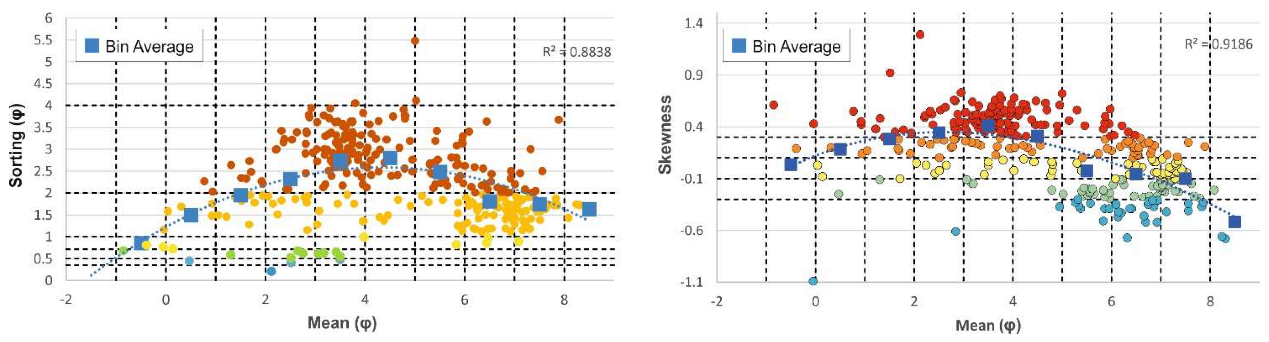
Figure 6 displays cross plots of the sorting coefficient, skewness, and mean diameter. Data were averaged within a range of one φ bin to identify any trends in these plots. The results demonstrate that the sorting coefficient decreases from −1φ to 5φ. Samples with mean grain sizes between −1φ and 0φ are moderately to very well sorted, while those ranging from 0φ to 5φ are poorly to very poorly sorted. Conversely, a better sorting trend is observed from 5φ to finer average values, resulting in a gradual improvement in the sorting of fine-grained sediments close to 1.5φ (poorly sorted). Furthermore, skewness exhibits a correlation with the mean grain diameter. Coarse-grained sediments (up to 0φ) are generally symmetrical, with a few outliers (2 samples) exhibiting strong negative or positive skewness. Up to 5φ, skewness shows a clear positive trend, as the examined samples generally have values greater than 0.3. However, skewness values decrease from 5φ to finer sediments, resulting in a coarse to strongly coarse skewed trend, as the samples exhibit finer average grain sizes.
3.3. Sediment Transport Patterns
Following Gao’s [36] methodology, a sediment transport map was designed with transport vectors in each sampling site. Before analyzing the vector transport directions, a statistical test for an assessment of the significance of the produced vectors was conducted in 246 out of 323 samples (covering the region Thasos—Alexandroupoli), by comparing the characteristic vector length of the analysis with the averages of randomly distributed samples in the study area. The characteristic vector length is practically the average length of the vectors that have been calculated for each sampling site and for the examined area, has a value of L = 1.9613. The process was based on the following steps: (a) using Excel Vba coding, each grain-size analysis was randomly reallocated in a different sampling site by generating a sequence of random numbers (1 to 246). If, for example, a sample numbered as 1 was located in a site with coordinates x: 610,969 and y: 4,529,442, by randomly assigning the number 63 it was reallocated in a site with coordinates x: 656,838 and y: 507,446. This process was repeated 100 times producing 100 randomly distributed datasets. (b) For each dataset transport vectors were produced and the average for each dataset was calculated. (c) The frequency of the 100 datasets (Figure 7a) was used to generate a normal distribution curve in order to calculate the critical values L90, L95, and L99 (Figure 7b,c,d respectively). The real dataset characteristic length was then statistically tested for significance with aforementioned critical values. According to the statistical test (Z test), the estimated transport vectors are significant in a 0.1 and 0.05 level (for 90% CI z = 4.13 > 1.645, 95% CI z = 2.69 > 1.96) and it is not significant for 0.01 level (for 99% CI z = 0.05 < 2.58). According to Davis [37] a confidence interval of 95% is acceptable for testing the significance of a dataset.
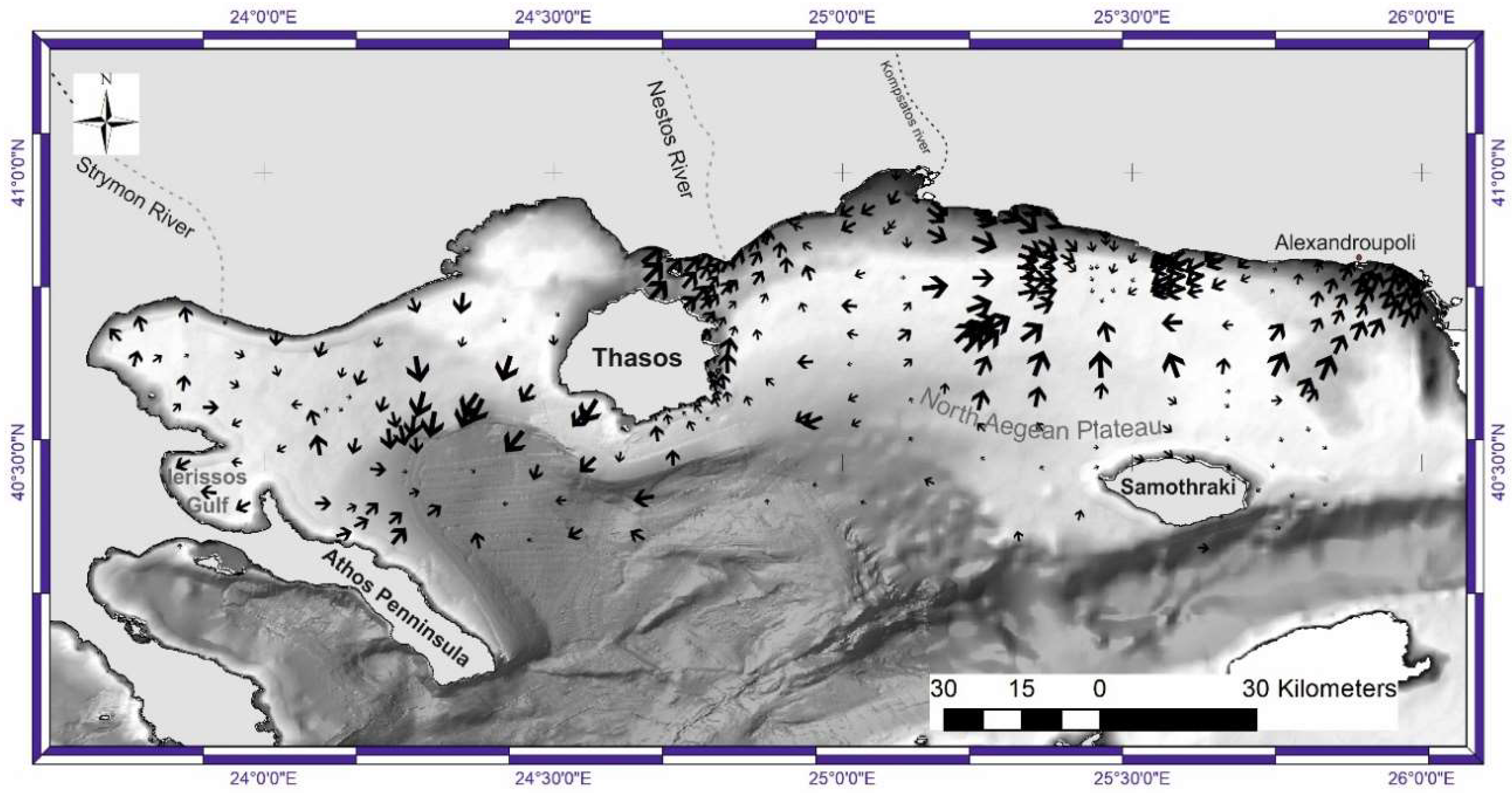
The analysis of grain-size trends has revealed a complex sediment transport network (Figure 8), highlighting the different processes that control sediment distribution in the marine environment. In the eastern part of the study area, sediment transport is mainly towards the north or northeast. Transport vectors are oriented towards the west or east near the coastal area. In the easternmost area, close to Alexandroupoli, the NNE trend is sustained for a long distance. Strong N-NE transport patterns have been identified along Thasos Island’s eastern and northern coastline. Thasos’s western and southwestern coasts show W-SW trends similar to the sediment transport vectors estimated for the open marine area westwards of Thasos. In the periphery of the semicircular depression defined by the Athos Peninsula and Thasos Island, the vector pattern is radial, with sediment transport directed towards the deepest central part of the depression. Between Thasos and Samothraki, especially near the margins of the North Aegean Plateau, sediment transport vectors are less significant, in terms of vector length.
The direction of sediment transport is not always the same as the direction of river flow, especially in areas near river deltas where sediment inflow is higher. For instance, in the Strymon River delta, the vectors indicating sediment transport have a weak tendency towards the south-southeast. On the other hand, in the Nestos River delta, sediment transport vectors are oriented towards the north-northeast. Finally, in the case of the Kompsatos River, net transport vectors align with the direction of sediment inflow.
4. Discussion
4.1. North Aegean Water Circulation Pattern
Various factors, such as sediment sources, hydrodynamic conditions, and topography features, influence the distribution of grain-size parameters in an area. In the Aegean region, the circulation pattern is driven by a thermohaline circulation close to the surface that involves the outflow of low-salinity water from the Black Sea (salinity ranging from 22.50 to 27.50 psu and an influx of 5.000 to 15.000 m3/s [38]) and the inflow of freshwater from rivers that flow into the Aegean [39] (Figure 9 and Figure 10). Additionally, the Aegean region receives saline water from the eastern Mediterranean. In the northern Aegean, the river runoff controls the sediment distribution in close sub-basins such as Thermaikos Gulf [40,41,42] which are not exposed neither to the open water’s circulation of the Aegean nor to the influx of Black Sea water masses. Studies conducted in the area [38] support the idea that the water masses from the Black Sea that enter the northern Aegean region dominate the combined effect of all freshwater influx (annual river water influx according to [38] has been estimated to 50 m3/s for Nestos and 100 m3/s for Strymonas and Evros respectively). This influx explains the lower salinities in northern Aegean [38,43,44,45]. Seasonal variations occur in the water circulation pattern. However, the general context is that the circulation in the Aegean Sea is controlled by the buoyancy input from the Black Sea to a lesser degree in North Aegean (except Thermaikos Gulf) by the river discharge, and the effects of winds in the region. The overall tendency of the buoyancy force is to create a cyclonic circulation around the Aegean. Another significant process is the transportation of dense waters formed on the shallow parts during the cold winter months that slowly descend toward the deep basins. According to [43], dense waters originating from the north Aegean shelf areas can generally remain in the adjacent deep basins for long periods. Due to their thickness, separating sills exceeding the bottom layer’s depth impede flow.
4.2. Water Circulation Pattern and Sediment Transport
Sediment transport patterns can provide insights into the complexity of water circulation and the influence of basin topography. The area located northwards of Samothraki Island, as defined by the direction of transport vectors, is predominantly influenced by the north Aegean gyre. The transport vectors exhibit a consistent N-NE orientation, which is aligned with the flow trend of the gyre in this specific area. The impact of the gyre is also reflected in the spatial distribution of sediment components and statistical parameters. The data suggest that sediments in the gyre area are predominantly sand, and skewness values are symmetrical or coarse skewed, indicating that fine fractions are transported northwards, following reworking. Near the coast, the impact of the gyre diminishes, and longshore drift becomes the dominant factor, as indicated by the transport vector trending parallel to the coast. A more complex and difficult-to-assess pattern regarding sediment transport is persistent in the area defined as NE of Samothraki to the Alexandroupoli coast. The dominant trend towards the northeast suggests that masses of low salinity, such as those dispersed in the area (Figure 10a,b), combined with the north Aegean gyre, result in a composite transport vector that forces fine-grained sediment towards the coast. This process is reflected in the increased clay component in the specific area (Figure 4).
In the studied region, sediment transport vectors exhibit bidirectional shifting towards the northwestern and northeastern directions between Samothraki and Thasos islands. A sector with less significant sediment transport vectors is identified where the BSW and North Aegean gyre are clearly separated and follow northwestern and northeastern directions, respectively. Sediment transport vectors become more intense in areas where the plume of low-salinity water expands on the shelf regions, and the depth decreases. Along the eastern coast of Thasos, BSW circulation is consistent with sediment transport vectors. On the northern coast of Samothraki, there is a complex situation where sediment transport vectors are moving towards the northeast despite the low-salinity plume expanding towards the west. This situation can be attributed to the combined effect of Nestos River’s outflow and the Black Sea Water (BSW) fluxes, resulting in a configuration that shifts the transport vectors towards the northeast.
The region between the Thasos and Athos Peninsula displays a radial pattern in the areas near the shelf break. The fine-grained sediment from the shelf (mainly silts) is re-deposited at the deeper parts of the morphological depression, where water circulation is reduced, and stagnant conditions are prevalent. This regime is also supported by the small length of the net transport vectors. This supports [43]’s hypothesis that dense waters formed in shallow areas during the cold winter months are transported to the deep sea, ultimately remaining in adjacent deep basins for prolonged periods due to the difficulty in flowing over separating sills that exceed the thickness of the bottom layers. Consequently, sediment transport vectors in the area are insignificant. At the open shelf to the coast region, sediment transport patterns are generally consistent with the flow trajectories proposed by [39]. The significance of net transport vectors may not be as prominent as those affected by BSW or North Aegean gyre. However, assessing the controlling factors that impact sediment dispersal is still essential. Close to the coast, the outflow of the Strymon River leads to a group of vectors trending towards the south, despite the fact that the length of the vectors indicates a weak trend of sediment reworking by this process. In Ierissos Gulf, the transport vectors steadily trend toward the W, consistent with the prevailing wind direction [48]. This results in a washout of the suspended fine-grained material, accumulating in the coastline, as indicated by the mean phi values in the specific area (Figure 5a). Lastly, the net transport vectors in the area defined by the northern coast of the Athos Peninsula (northwards of Ierissos Gulf) reflect the outflow of two local-scale river streams, resulting in N or NE directions.
5. Conclusions
Multiple factors, such as the sources of sediment, hydrodynamic conditions, and topographical features, influence the distribution of grain-size parameters in a particular area. The complex net sediment transport patterns in the North Aegean basin have been identified by analyzing statistical parameters like mean size, sorting, and skewness. These patterns reveal the contribution of various hydrodynamic factors and their impact on the area.
The sediment distribution in the central and eastern parts of the study area is primarily influenced by two factors, namely, the north Aegean gyre and the Black Sea water mass (BSW), which enters the Aegean space through the Marmara Sea. The BSW, characterized by low-salinity waters, generates a plume that spreads towards the W-NW. As this plume reaches lower depths at the shelf areas, it triggers a reworking of basin floor sediments, reflected in the measured net transport vectors. The north Aegean gyre also favors sediment reworking, as net transport vectors are generally oriented with the direction of the gyre. In the shallow water coastal areas, the dominant process is the longshore drift, which is indicated by vectors that trend parallel to the coast.
The net transport vectors are insignificant in the deeper parts of the basin beyond the shelf edge, indicating the formation of stagnant conditions. This is due to the gradual movement of cold, dense waters downslope, which become trapped in the deeper parts and remain there for long periods. This process helps to maintain the initial textural characteristics of the accumulated sediments on the basin floor, preventing further reworking.
In the western part of the study area, two processes dominate the sediment distribution pattern. Near the shelf edge, the circulation of bottom seawater (BSW) plays a significant role, while in the shelf–coastal areas, the outflow of rivers is more important. In small gulfs such as Ierissos, the direction of prevailing winds also contributes to sediment distribution.
Regarding the significance of sediment distribution patterns, the area where transport vectors suggest the intense reworking of sediments could potentially favor the enrichment of sediment in placers, considering that minerals are not so mobile. Such an area has been identified northwestern of Samothraki, where sand component is dominant implying the wash out of finer material. The composition of placers in the specific area is under research. Sediment transport is also important in terms of the existing and planned infrastructures. The eastern part of the study area accommodates underwater cable systems for telecommunications and electric energy transport, while a major cable project is planned for the connection of the northeastern Aegean islands with the National System of Electricity Transport. Finally, the identification of the seafloor sediment dynamics in this area is crucial given that in the easternmost part of the Samothraki–Alexandroupoli shelf is a priority area for the potential installation of anchored offshore windfarms, and thus desktop studies for underwater foundations and electricity transport are in progress. Sediment transport vectors can help identify areas where cables or the foundation of the aforementioned infrastructures can be exposed or even damaged by intense sediment reworking.
Author Contributions
Conceptualization, I.V. and I.Z.; methodology, I.V. and I.Z.; validation, I.V. and I.Z.; data curation, I.V. and I.Z.; writing—original draft preparation, I.V. and I.Z.; writing—review and editing, I.V. and I.Z.; visualization, I.V. and I.Z. All authors have read and agreed to the published version of the manuscript.
Funding
This research was funded by NSRF 2014–2020, grant number 5030010 (“Geological Mapping of Greece for the support of innovation and entrepreneurship—GEOINFRA”), and European Commission contract No. SI2.658129 (“European Marine Observation and Data Network—Lot 2 Geology”). The APC was funded by European Commission contract No. SI2.658129 (“European Marine Observation and Data Network—Lot 2 Geology”).
Institutional Review Board Statement
Not applicable.
Informed Consent Statement
Not applicable.
Data Availability Statement
Data is contained within the article.
Acknowledgments
Used data were collected in the frame of the Research and Development program of the European Communities (E.E.E., 1984–1989) and the NSRF/Operational Programme Competitiveness & Entrepreneurship (2013–2015), project No. 351008 (“YPOTHER: Marine geology and mineral research study along the coastline between Chalkidiki and Kavala, and the caldera of Santorini”).
Conflicts of Interest
The authors declare no conflicts of interest.
Appendix A

Table A1.
Grain-size parameters.
| ID | x | y | Mean | Sort | Skew |
|---|---|---|---|---|---|
| 1 | 564,117 | 4,495,734 | 2.12 | 0.21 | 1.29 |
| 2 | 565,142 | 4,499,443 | 2.51 | 0.41 | 0.1 |
| 3 | 564,877 | 4,502,987 | 0.47 | 0.45 | −0.25 |
| 4 | 664,621 | 4,521,654 | 3.5 | 0.48 | 0.06 |
| 5 | 561,735 | 4,513,753 | 2.51 | 0.52 | −0.02 |
| 6 | 662,132 | 4,522,987 | 3.5 | 0.55 | 0.03 |
| 7 | 572,623 | 4,526,958 | 1.3 | 0.59 | −0.11 |
| 8 | 564,133 | 4,507,607 | 3.06 | 0.61 | −0.11 |
| 9 | 561,072 | 4,494,629 | 2.75 | 0.62 | 0.2 |
| 10 | 571,002 | 4,525,247 | 3.17 | 0.63 | −0.15 |
| 11 | 604,855 | 4,531,510 | 3.42 | 0.65 | −0.06 |
| 12 | 622,224 | 4,528,077 | −0.85 | 0.68 | 0.61 |
| 13 | 568,684 | 4,522,757 | 2.65 | 0.68 | 0.03 |
| 14 | 584,505 | 4,531,557 | 0.14 | 0.72 | −0.08 |
| 15 | 632,223 | 4,485,682 | −0.05 | 0.77 | −1.09 |
| 16 | 627,886 | 4,484,681 | −0.39 | 0.81 | 0.19 |
| 17 | 538,723.7 | 4,468,109 | 5.83 | 0.82 | 0.38 |
| 18 | 530,532.2 | 4,481,180 | 6.44 | 0.86 | 0.2 |
| 19 | 620,525 | 4,518,866 | 7.08 | 0.89 | −0.23 |
| 20 | 520,544.2 | 4,481,179 | 6.47 | 0.97 | 0.2 |
| 21 | 653,457 | 4,523,264 | 3.98 | 0.99 | 0.32 |
| 22 | 543,395.6 | 4,475,578 | 6.34 | 1.11 | 0.26 |
| 23 | 515,674.6 | 4,474,244 | 6.34 | 1.12 | 0.04 |
| 24 | 536,425.5 | 4,486,993 | 6.92 | 1.12 | −0.52 |
| 25 | 539,524.2 | 4,480,960 | 5.95 | 1.13 | 0.43 |
| 26 | 576,686 | 4,530,084 | 2.84 | 1.15 | −0.61 |
| 27 | 599,227 | 4,497,661 | 7.16 | 1.15 | −0.16 |
| 28 | 643,503 | 4,480,647 | −0.04 | 1.16 | 0.43 |
| 29 | 516,552.9 | 4,481,735 | 6.22 | 1.17 | −0.11 |
| 30 | 621,283 | 4,521,277 | 7.3 | 1.18 | 0.05 |
| 31 | 620,447 | 4,521,096 | 7.31 | 1.18 | 0.03 |
| 32 | 521,826.1 | 4,477,227 | 6.46 | 1.18 | 0.15 |
| 33 | 580,491 | 4,479,024 | 6.82 | 1.19 | 0.09 |
| 34 | 524,872.9 | 4,473,734 | 6.18 | 1.19 | 0.21 |
| 35 | 507,686.6 | 4,486,452 | 6.54 | 1.19 | 0.12 |
| 36 | 579,912 | 4,491,104 | 5.86 | 1.25 | −0.39 |
| 37 | 614,096 | 4,525,320 | 7.23 | 1.26 | −0.12 |
| 38 | 545,347.7 | 4,469,495 | 5.98 | 1.27 | 0.31 |
| 39 | 650,533 | 4,477,987 | 1.67 | 1.28 | 0.19 |
| 40 | 565,173 | 4,522,571 | 3.04 | 1.28 | 0.26 |
| 41 | 504,645.3 | 4,493,972 | 7 | 1.28 | −0.18 |
| 42 | 573,619 | 4,475,900 | 7.21 | 1.29 | 0 |
| 43 | 617,571 | 4,521,085 | 7.22 | 1.31 | −0.11 |
| 44 | 531,091.4 | 4,468,284 | 6.05 | 1.32 | 0.32 |
| 45 | 597,344 | 4,479,903 | 6.98 | 1.34 | −0.2 |
| 46 | 668,092 | 4,518,492 | 3.95 | 1.35 | 0.54 |
| 47 | 657,933 | 4,522,124 | 3.97 | 1.36 | 0.57 |
| 48 | 660,789 | 4,520,088 | 4.38 | 1.37 | 0.47 |
| 49 | 491,560.1 | 4,477,278 | 7.18 | 1.37 | 0.01 |
| 50 | 664,646 | 4,514,250 | 7.51 | 1.38 | −0.09 |
| 51 | 492,158.7 | 4,493,472 | 7.16 | 1.38 | −0.07 |
| 52 | 512,381.4 | 4,495,458 | 6.82 | 1.4 | 0.18 |
| 53 | 481,810.7 | 4,509,859 | 7.33 | 1.41 | 0.11 |
| 54 | 522,251.5 | 4,500,630 | 6.28 | 1.42 | 0.24 |
| 55 | 656,900 | 4,515,623 | 8.08 | 1.43 | −0.21 |
| 56 | 487,873.2 | 4,482,525 | 7 | 1.44 | −0.19 |
| 57 | 657,604 | 4,521,038 | 4.29 | 1.45 | 0.56 |
| 58 | 631,609 | 4,472,824 | 1.22 | 1.46 | 0.38 |
| 59 | 626,452 | 4,518,931 | 6.86 | 1.46 | −0.37 |
| 60 | 635,417 | 4,484,814 | 0.92 | 1.48 | 0.45 |
| 61 | 591,374 | 4,534,106 | 1.05 | 1.49 | 0.17 |
| 62 | 558,846 | 4,493,686 | 4.46 | 1.49 | 0.42 |
| 63 | 554,411.7 | 4,469,214 | 6.58 | 1.49 | 0.29 |
| 64 | 535,054.8 | 4,475,005 | 6.42 | 1.5 | 0.24 |
| 65 | 542,773.5 | 4,511,316 | 2.24 | 1.51 | 0.03 |
| 66 | 587,523 | 4,475,865 | 5.86 | 1.54 | −0.28 |
| 67 | 522,080 | 4,486,185 | 6.88 | 1.55 | −0.04 |
| 68 | 663,687 | 4,516,233 | 7.15 | 1.57 | −0.06 |
| 69 | 598,300 | 4,532,038 | 0.04 | 1.58 | 0.03 |
| 70 | 586,382 | 4,490,871 | 7.45 | 1.58 | −0.03 |
| 71 | 668,183 | 4,514,483 | 7.52 | 1.58 | −0.04 |
| 72 | 566,111 | 4,496,214 | 3.08 | 1.59 | 0.35 |
| 73 | 478,119.4 | 4,507,424 | 7.23 | 1.59 | −0.05 |
| 74 | 594,319 | 4,495,593 | 6.25 | 1.6 | −0.16 |
| 75 | 585,973 | 4,495,801 | 6.93 | 1.6 | −0.31 |
| 76 | 496,246.8 | 4,503,711 | 6.83 | 1.61 | −0.17 |
| 77 | 495,485.8 | 4,497,867 | 7.03 | 1.62 | −0.21 |
| 78 | 575,958 | 4,521,287 | 7.62 | 1.63 | −0.15 |
| 79 | 647,569 | 4,483,503 | 7.38 | 1.67 | −0.11 |
| 80 | 508,892 | 4,493,121 | 6.68 | 1.67 | 0.24 |
| 81 | 648,567 | 4,471,734 | 6.87 | 1.68 | 0.22 |
| 82 | 608,251 | 4,531,252 | 0.31 | 1.69 | 0.2 |
| 83 | 630,399 | 4,521,338 | 6.32 | 1.69 | −0.67 |
| 84 | 501,636.3 | 4,500,436 | 6.99 | 1.69 | −0.11 |
| 85 | 666,081 | 4,516,162 | 7.56 | 1.7 | −0.34 |
| 86 | 487,496.9 | 4,466,948 | 4.91 | 1.7 | 0.35 |
| 87 | 516,467.1 | 4,506,008 | 6.62 | 1.7 | 0.01 |
| 88 | 632,470 | 4,523,336 | 6.45 | 1.71 | −0.06 |
| 89 | 508,583.4 | 4,475,158 | 6.08 | 1.71 | −0.1 |
| 90 | 650,488 | 4,519,531 | 7.79 | 1.72 | −0.29 |
| 91 | 648,645 | 4,488,614 | 7.86 | 1.72 | −0.33 |
| 92 | 612,766 | 4,518,982 | 8.31 | 1.72 | −0.68 |
| 93 | 513,830 | 4,499,073 | 6.92 | 1.72 | −0.04 |
| 94 | 571,450 | 4,522,476 | 7.06 | 1.73 | −0.05 |
| 95 | 480,993.8 | 4,502,872 | 7.03 | 1.73 | −0.16 |
| 96 | 666,463 | 4,512,746 | 7.56 | 1.74 | −0.41 |
| 97 | 660,582 | 4,516,689 | 7.67 | 1.74 | −0.27 |
| 98 | 594,415 | 4,488,039 | 8.24 | 1.74 | −0.66 |
| 99 | 511,084.8 | 4,492,952 | 6.18 | 1.74 | −0.11 |
| 100 | 641,097 | 4,482,959 | 0.93 | 1.75 | 0.42 |
| 101 | 563,372 | 4,494,956 | 3.45 | 1.75 | 0.47 |
| 102 | 565,626 | 4,497,906 | 3.78 | 1.75 | 0.34 |
| 103 | 495,900.1 | 4,482,883 | 2.15 | 1.75 | 0.25 |
| 104 | 632,567 | 4,516,899 | 2.83 | 1.78 | 0.28 |
| 105 | 614,182 | 4,518,784 | 6.83 | 1.78 | −0.31 |
| 106 | 524,392 | 4,490,001 | 1.78 | 1.78 | 0.37 |
| 107 | 494,219.2 | 4,509,572 | 5.87 | 1.78 | 0.28 |
| 108 | 614,211 | 4,516,588 | 6.14 | 1.79 | −0.42 |
| 109 | 519,773.5 | 4,469,054 | 5.27 | 1.79 | −0.33 |
| 110 | 496,666.2 | 4,474,488 | 7.06 | 1.8 | −0.08 |
| 111 | 519,143 | 4,472,329 | 6.55 | 1.81 | 0.2 |
| 112 | 547,067.3 | 4,482,398 | 1.52 | 1.82 | 0.29 |
| 113 | 535,175.7 | 4,500,982 | 2.32 | 1.83 | 0.23 |
| 114 | 512,642.3 | 4,474,267 | 6.5 | 1.83 | 0.03 |
| 115 | 661,975 | 4,519,435 | 4.66 | 1.84 | 0.63 |
| 116 | 667,413 | 4,517,396 | 7.16 | 1.84 | −0.04 |
| 117 | 511,540.7 | 4,469,297 | 5.56 | 1.84 | −0.23 |
| 118 | 647,640 | 4,509,570 | 2.6 | 1.86 | 0.27 |
| 119 | 578,494 | 4,491,862 | 6.66 | 1.86 | −0.46 |
| 120 | 574,990 | 4,524,299 | 7.13 | 1.86 | 0.13 |
| 121 | 630,052 | 4,522,196 | 7.83 | 1.87 | −0.37 |
| 122 | 556,389 | 4,523,023 | 6.03 | 1.89 | −0.16 |
| 123 | 623,600 | 4,521,188 | 6.79 | 1.89 | 0.14 |
| 124 | 630,593 | 4,516,862 | 2.78 | 1.9 | 0.21 |
| 125 | 664,328 | 4,519,024 | 6.48 | 1.9 | 0.32 |
| 126 | 610,969 | 4,529,442 | 7.29 | 1.9 | −0.1 |
| 127 | 528,753.8 | 4,506,074 | 1.39 | 1.9 | 0.3 |
| 128 | 611,368 | 4,516,528 | 6.69 | 1.91 | −0.52 |
| 129 | 570,588 | 4,495,021 | 7.29 | 1.91 | −0.22 |
| 130 | 655,432 | 4,518,522 | 7.33 | 1.91 | −0.04 |
| 131 | 562,258 | 4,521,312 | 7.03 | 1.92 | 0.09 |
| 132 | 541,984.6 | 4,506,608 | 2.05 | 1.92 | 0.05 |
| 133 | 635,420 | 4,516,931 | 2.85 | 1.93 | 0.35 |
| 134 | 563,884 | 4,522,714 | 5.14 | 1.93 | 0.46 |
| 135 | 655,327 | 4,476,332 | 1.94 | 1.94 | 0.34 |
| 136 | 488,431 | 4,511,368 | 7.35 | 1.94 | 0.07 |
| 137 | 655,058 | 4,502,781 | 1.69 | 1.95 | 0.17 |
| 138 | 561,205 | 4,492,780 | 6.75 | 1.95 | −0.32 |
| 139 | 577,404 | 4,528,550 | 3.64 | 1.96 | 0.66 |
| 140 | 506,877.7 | 4,491,552 | 6.36 | 1.96 | −0.06 |
| 141 | 565,310 | 4,520,260 | 6.21 | 2.01 | 0.41 |
| 142 | 564,144 | 4,519,787 | 6.86 | 2.01 | 0.06 |
| 143 | 568,149 | 4,517,201 | 6.89 | 2.01 | 0.06 |
| 144 | 666,286 | 4,520,610 | 7.36 | 2.01 | −0.23 |
| 145 | 665,721 | 4,519,672 | 6.76 | 2.02 | 0.25 |
| 146 | 487,116.7 | 4,493,485 | 6.74 | 2.02 | −0.35 |
| 147 | 610,429 | 4,469,538 | 0.94 | 2.03 | 0.14 |
| 148 | 611,256 | 4,522,984 | 7.42 | 2.05 | −0.01 |
| 149 | 604,820 | 4,525,805 | 2.42 | 2.08 | −0.05 |
| 150 | 622,653 | 4,509,270 | 2.46 | 2.08 | 0.28 |
| 151 | 647,168 | 4,521,439 | 7.21 | 2.08 | −0.12 |
| 152 | 508,000.7 | 4,504,417 | 6.46 | 2.08 | −0.27 |
| 153 | 495,954.8 | 4,490,603 | 6.77 | 2.1 | −0.27 |
| 154 | 514,094.7 | 4,471,404 | 5.37 | 2.11 | −0.39 |
| 155 | 563,198 | 4,493,413 | 6.66 | 2.12 | −0.28 |
| 156 | 592,967 | 4,519,015 | 3.16 | 2.13 | 0.25 |
| 157 | 558,864 | 4,491,374 | 4.03 | 2.13 | 0.68 |
| 158 | 562,284 | 4,490,167 | 6.13 | 2.14 | −0.47 |
| 159 | 640,251 | 4,473,889 | 3.55 | 2.17 | 0.54 |
| 160 | 659,649 | 4,518,612 | 6.34 | 2.17 | 0.35 |
| 161 | 555,381.1 | 4,476,142 | 5.65 | 2.17 | −0.25 |
| 162 | 632,126 | 4,510,975 | 3.2 | 2.2 | 0.48 |
| 163 | 613,319 | 4,490,460 | 6.41 | 2.2 | −0.39 |
| 164 | 626,330 | 4,523,199 | 7.01 | 2.2 | −0.06 |
| 165 | 517,027.2 | 4,494,024 | 5.41 | 2.2 | −0.27 |
| 166 | 518,255.9 | 4,487,260 | 3.95 | 2.2 | 0.51 |
| 167 | 653,480 | 4,510,892 | 1.95 | 2.21 | 0.33 |
| 168 | 653,369 | 4,521,874 | 5.97 | 2.22 | 0.57 |
| 169 | 521,592.5 | 4,489,595 | 5.52 | 2.23 | −0.2 |
| 170 | 573,213 | 4,526,501 | 6.53 | 2.26 | 0.13 |
| 171 | 645,558 | 4,478,932 | 0.77 | 2.27 | 0.55 |
| 172 | 648,115 | 4,503,411 | 1.92 | 2.27 | 0.14 |
| 173 | 585,313 | 4,502,114 | 5.61 | 2.3 | −0.2 |
| 174 | 566,119 | 4,521,655 | 5.86 | 2.32 | 0.44 |
| 175 | 653,055 | 4,497,342 | 1.61 | 2.33 | 0.35 |
| 176 | 557,240 | 4,488,739 | 6.92 | 2.33 | −0.27 |
| 177 | 652,048 | 4,499,290 | 1.51 | 2.34 | 0.92 |
| 178 | 659,594 | 4,510,281 | 2.53 | 2.35 | 0.33 |
| 179 | 522,659.1 | 4,493,944 | 3.93 | 2.36 | 0.19 |
| 180 | 632,512 | 4,519,078 | 4.53 | 2.39 | 0.29 |
| 181 | 611,622 | 4,532,691 | 5.91 | 2.39 | 0.19 |
| 182 | 530,854.5 | 4,492,842 | 3.33 | 2.39 | 0.45 |
| 183 | 623,743 | 4,516,775 | 4.12 | 2.41 | 0.56 |
| 184 | 604,936 | 4,484,479 | 4.65 | 2.41 | 0.42 |
| 185 | 573,729 | 4,498,731 | 5.56 | 2.43 | −0.24 |
| 186 | 591,669 | 4,538,582 | 6.54 | 2.43 | 0.17 |
| 187 | 511,161.2 | 4,500,122 | 5.34 | 2.44 | −0.36 |
| 188 | 567,463 | 4,502,548 | 2.81 | 2.45 | 0.66 |
| 189 | 579,136 | 4,519,779 | 3.63 | 2.45 | 0.49 |
| 190 | 642,988 | 4,519,506 | 5.52 | 2.45 | −0.26 |
| 191 | 622,254 | 4,497,850 | 7.11 | 2.45 | −0.42 |
| 192 | 638,909 | 4,518,349 | 3.83 | 2.46 | 0.56 |
| 193 | 620,555 | 4,516,660 | 5.32 | 2.46 | −0.3 |
| 194 | 620,429 | 4,525,387 | 1.71 | 2.48 | −0.1 |
| 195 | 635,385 | 4,519,172 | 4.27 | 2.49 | 0.31 |
| 196 | 556,978 | 4,492,129 | 4.95 | 2.49 | 0.61 |
| 197 | 630,509 | 4,519,024 | 5.57 | 2.5 | −0.34 |
| 198 | 591,201 | 4,529,171 | 6.93 | 2.5 | −0.17 |
| 199 | 637,608 | 4,467,992 | 7.56 | 2.5 | 0.25 |
| 200 | 604,362 | 4,508,527 | 3.27 | 2.51 | 0.52 |
| 201 | 638,245 | 4,522,501 | 6.37 | 2.56 | −0.39 |
| 202 | 502,374.4 | 4,485,617 | 4.79 | 2.56 | −0.21 |
| 203 | 545,862.2 | 4,491,199 | 4.04 | 2.58 | 0.2 |
| 204 | 604,921 | 4,510,478 | 3.4 | 2.59 | 0.48 |
| 205 | 626,339 | 4,523,198 | 6.2 | 2.59 | −0.43 |
| 206 | 520,131.9 | 4,487,833 | 3.55 | 2.59 | 0.53 |
| 207 | 528,672.6 | 4,513,176 | 3.5 | 2.6 | 0.53 |
| 208 | 621,423 | 4,491,206 | 6 | 2.62 | 0.17 |
| 209 | 512,939.9 | 4,485,970 | 3.58 | 2.62 | 0.6 |
| 210 | 626,446 | 4,516,814 | 3.97 | 2.63 | 0.62 |
| 211 | 565,216 | 4,517,792 | 5.83 | 2.63 | −0.21 |
| 212 | 641,092 | 4,483,531 | 1.31 | 2.64 | 0.48 |
| 213 | 547,375.6 | 4,492,928 | 5.3 | 2.65 | 0.56 |
| 214 | 534,941.5 | 4,510,079 | 5.39 | 2.66 | −0.02 |
| 215 | 501,634.8 | 4,506,610 | 5.87 | 2.66 | 0.5 |
| 216 | 633,234 | 4,522,204 | 5.3 | 2.67 | 0.05 |
| 217 | 551,867.5 | 4,484,249 | 3.35 | 2.68 | 0.22 |
| 218 | 614,114 | 4,523,035 | 4.39 | 2.69 | 0.16 |
| 219 | 614,113 | 4,523,018 | 5.4 | 2.7 | −0.22 |
| 220 | 602,250 | 4,508,497 | 3.04 | 2.72 | 0.54 |
| 221 | 529,344.6 | 4,491,880 | 3.65 | 2.72 | 0.5 |
| 222 | 656,838 | 4,507,446 | 1.68 | 2.73 | 0.28 |
| 223 | 621,974 | 4,514,811 | 4.57 | 2.73 | 0.42 |
| 224 | 597,796 | 4,517,072 | 4.11 | 2.75 | 0.51 |
| 225 | 488,571.2 | 4,503,505 | 3.31 | 2.75 | 0.6 |
| 226 | 586,635 | 4,519,554 | 3.64 | 2.76 | 0.41 |
| 227 | 585,064 | 4,513,522 | 3.86 | 2.76 | 0.35 |
| 228 | 621,909 | 4,483,040 | 5.46 | 2.76 | 0.41 |
| 229 | 529,860.2 | 4,494,108 | 4.95 | 2.76 | −0.37 |
| 230 | 518,943.6 | 4,490,862 | 3.85 | 2.76 | 0.53 |
| 231 | 652,603 | 4,490,698 | 3.64 | 2.77 | 0.57 |
| 232 | 564,741 | 4,491,576 | 5.83 | 2.8 | −0.51 |
| 233 | 567,407 | 4,521,513 | 5.73 | 2.81 | 0.14 |
| 234 | 567,372 | 4,516,785 | 3.19 | 2.87 | 0.51 |
| 235 | 585,715 | 4,507,979 | 3.87 | 2.87 | 0.53 |
| 236 | 565,888 | 4,494,824 | 4.21 | 2.87 | 0.62 |
| 237 | 630,250 | 4,517,573 | 4.47 | 2.87 | 0.65 |
| 238 | 578,732 | 4,502,659 | 4.21 | 2.88 | 0.22 |
| 239 | 603,449 | 4,506,664 | 2.8 | 2.9 | 0.44 |
| 240 | 640,464 | 4,510,512 | 3.75 | 2.9 | 0.55 |
| 241 | 646,896 | 4,517,422 | 3.35 | 2.91 | 0.39 |
| 242 | 659,987 | 4,513,777 | 2.95 | 2.92 | 0.73 |
| 243 | 594,648 | 4,533,994 | 4.02 | 2.92 | −0.02 |
| 244 | 521,812 | 4,512,913 | 3.49 | 2.93 | 0.41 |
| 245 | 604,173 | 4,513,613 | 3.63 | 2.94 | 0.51 |
| 246 | 612,755 | 4,496,621 | 3.75 | 2.94 | 0.52 |
| 247 | 613,552 | 4,482,908 | 4.03 | 2.98 | 0.33 |
| 248 | 647,904 | 4,496,312 | 2.21 | 2.99 | 0.49 |
| 249 | 611,303 | 4,522,959 | 3.24 | 2.99 | 0.44 |
| 250 | 619,349 | 4,473,746 | 4.3 | 2.99 | 0.2 |
| 251 | 614,931 | 4,530,428 | 2.22 | 3 | 0.51 |
| 252 | 640,821 | 4,497,870 | 3.03 | 3 | 0.44 |
| 253 | 559,746 | 4,484,134 | 3.18 | 3 | 0.64 |
| 254 | 632,495 | 4,521,390 | 7.32 | 3 | −0.03 |
| 255 | 593,507 | 4,513,315 | 3.65 | 3.02 | 0.13 |
| 256 | 605,668 | 4,507,465 | 3.68 | 3.02 | 0.21 |
| 257 | 621,730 | 4,486,738 | 4.05 | 3.03 | 0.41 |
| 258 | 621,939 | 4,502,781 | 4.69 | 3.03 | 0.56 |
| 259 | 653,374 | 4,516,012 | 3.48 | 3.06 | 0.5 |
| 260 | 567,524 | 4,495,917 | 5.84 | 3.08 | −0.22 |
| 261 | 662,166 | 4,510,707 | 3.89 | 3.09 | 0.44 |
| 262 | 614,143 | 4,521,038 | 2.81 | 3.12 | 0.28 |
| 263 | 571,767 | 4,518,778 | 3.74 | 3.12 | 0.61 |
| 264 | 613,663 | 4,514,060 | 5.96 | 3.13 | −0.24 |
| 265 | 559,636 | 4,521,105 | 3.41 | 3.15 | 0.49 |
| 266 | 598,017 | 4,526,945 | 2.36 | 3.16 | 0.52 |
| 267 | 567,672 | 4,505,479 | 3.46 | 3.16 | 0.37 |
| 268 | 571,757 | 4,507,677 | 4.9 | 3.19 | 0.41 |
| 269 | 630,426 | 4,523,290 | 5.41 | 3.19 | 0.1 |
| 270 | 616,905 | 4,522,819 | 5.95 | 3.19 | −0.39 |
| 271 | 578,964 | 4,524,866 | 3.74 | 3.21 | 0.7 |
| 272 | 647,840 | 4,522,994 | 2.53 | 3.22 | 0.56 |
| 273 | 587,542 | 4,531,902 | 3.57 | 3.22 | 0.59 |
| 274 | 578,506 | 4,512,987 | 4.43 | 3.22 | 0.06 |
| 275 | 604,918 | 4,502,365 | 2.38 | 3.23 | 0.42 |
| 276 | 656,495 | 4,512,529 | 3.59 | 3.24 | 0.37 |
| 277 | 607,033 | 4,510,416 | 4.22 | 3.24 | 0.09 |
| 278 | 640,020 | 4,502,944 | 3.67 | 3.29 | 0.42 |
| 279 | 638,097 | 4,524,193 | 3.2 | 3.3 | −0.15 |
| 280 | 635,352 | 4,521,380 | 5.96 | 3.3 | −0.29 |
| 281 | 564,879 | 4,516,093 | 3.92 | 3.32 | 0.42 |
| 282 | 538,150.4 | 4,496,083 | 3.42 | 3.32 | 0.35 |
| 283 | 593,457 | 4,508,072 | 3.69 | 3.33 | 0.51 |
| 284 | 632,019 | 4,490,614 | 3.26 | 3.34 | 0.24 |
| 285 | 566,909 | 4,498,842 | 3.6 | 3.34 | 0.44 |
| 286 | 611,984 | 4,508,792 | 3.77 | 3.34 | 0.67 |
| 287 | 488,069.3 | 4,498,286 | 4.13 | 3.35 | 0.53 |
| 288 | 611,214 | 4,519,012 | 2.83 | 3.37 | 0.65 |
| 289 | 565,246 | 4,514,399 | 3.32 | 3.38 | 0.42 |
| 290 | 564,313 | 4,513,775 | 2.63 | 3.39 | 0.59 |
| 291 | 640,879 | 4,488,617 | 3.75 | 3.39 | 0.36 |
| 292 | 617,501 | 4,525,368 | 2.82 | 3.4 | 0.39 |
| 293 | 557,261 | 4,516,246 | 6.09 | 3.4 | −0.35 |
| 294 | 630,490 | 4,523,901 | 2.32 | 3.42 | 0.55 |
| 295 | 572,626 | 4,514,777 | 5.44 | 3.42 | −0.19 |
| 296 | 640,756 | 4,495,092 | 3.61 | 3.49 | 0.4 |
| 297 | 604,800 | 4,519,018 | 3.56 | 3.53 | 0.44 |
| 298 | 563,477 | 4,515,618 | 4.09 | 3.57 | 0.31 |
| 299 | 562,048 | 4,518,381 | 3.55 | 3.58 | 0.46 |
| 300 | 611,863 | 4,524,520 | 3.04 | 3.62 | 0.38 |
| 301 | 593,760 | 4,502,678 | 3.4 | 3.62 | 0.51 |
| 302 | 604,735 | 4,490,334 | 3.74 | 3.62 | 0.29 |
| 303 | 604,659 | 4,495,731 | 3.45 | 3.63 | 0.49 |
| 304 | 632,621 | 4,502,964 | 3.71 | 3.63 | 0.44 |
| 305 | 584,773 | 4,528,631 | 3.75 | 3.63 | 0.44 |
| 306 | 655,149 | 4,487,373 | 6.44 | 3.63 | 0.1 |
| 307 | 484,153.2 | 4,502,856 | 4.27 | 3.64 | 0.61 |
| 308 | 590,532 | 4,528,047 | 7.89 | 3.67 | 0.21 |
| 309 | 597,731 | 4,530,796 | 4.8 | 3.7 | −0.02 |
| 310 | 604,871 | 4,530,432 | 3.28 | 3.71 | 0.46 |
| 311 | 603,649 | 4,509,133 | 2.88 | 3.73 | 0.52 |
| 312 | 622,366 | 4,526,538 | 4.56 | 3.75 | 0.22 |
| 313 | 564,689 | 4,511,003 | 4.81 | 3.76 | 0.04 |
| 314 | 568,067 | 4,513,500 | 3.17 | 3.77 | 0.47 |
| 315 | 613,013 | 4,502,793 | 4.79 | 3.77 | 0.06 |
| 316 | 623,499 | 4,525,449 | 2.87 | 3.78 | 0.38 |
| 317 | 566,690 | 4,510,249 | 3.96 | 3.83 | 0.36 |
| 318 | 556,672 | 4,519,694 | 4.77 | 3.9 | −0.07 |
| 319 | 568,349 | 4,508,414 | 3.3 | 3.93 | 0.39 |
| 320 | 593,469 | 4,525,652 | 2.92 | 3.94 | 0.45 |
| 321 | 642,416 | 4,522,487 | 3.8 | 4.05 | 0.08 |
| 322 | 632,510 | 4,496,022 | 5.02 | 4.11 | −0.25 |
| 323 | 611,297 | 4,521,007 | 5 | 5.48 | 0.72 |
References
- Atkins, R.J. Sediment Suspension by Waves. In Encyclopedia of Coastal Science; Schwartz, M.L., Ed.; Springer: Dordrecht, The Netherlands, 2005; pp. 850–853. [Google Scholar]
- Bagnold, R.J. Mechanics of marine sedimentation. Sea 1963, 3, 507–528. [Google Scholar]
- Middleton, G.V.; Hampton, M.A. Part I. Sediment Gravity Flows: Mechanics of Flow and Deposition; SEPM: Tulsa, OK, USA, 1973. [Google Scholar]
- Cieśla, M.; Gruca-Rokosz, R.; Bartoszek, L. Significance of organic matter in the process of aggregation of suspended sediments in retention reservoirs. Sci. Total Environ. 2022, 815, 152850. [Google Scholar] [CrossRef]
- Lee, B.J.; Kim, J.; Hur, J.; Choi, I.H.; Toorman, E.A.; Fettweis, M.; Choi, J.W. Seasonal Dynamics of Organic Matter Composition and Its Effects on Suspended Sediment Flocculation in River Water. Water Resour. Res. 2019, 55, 6968–6985. [Google Scholar] [CrossRef]
- Pettijohn, F.; Potter, P.E.; Siever, R. Transport, Deposition, and Deformation of Sand. In Sand and Sandstone; Springer: New York, NY, USA, 1972; pp. 327–382. [Google Scholar]
- McLaren, P. An interpretation of trends in grain size measurements. J. Sediment. Petrol. 1981, 51, 611–624. [Google Scholar]
- McLaren, P.; Bowles, D. The effects of sediment transport on grain-size distribution. J. Sediment. Petrol. 1985, 55, 457–470. [Google Scholar]
- Gao, S.; Collins, M. Net sediment transport patterns inferred from grain-size trends, based upon definition of “transport vectors”. Sediment. Geol. 1992, 81, 47–60. [Google Scholar] [CrossRef]
- Zananiri, Ι.; Mitropoulos, D.; Zimianitis, V.; Ioakim, C.; Papadopoulos, V.; Efthimiou, G. Marine geology data accessibility in the European Framework: The I.G.M.E. participation in the GEO-SEAS project. Bull. Geol. Soc. Greece 2016, 47, 1590–1597. [Google Scholar] [CrossRef]
- Folk, R.L. The distinction between grain size and mineral composition in sedimentary rock nomenclature. J. Geol. 1954, 62, 344–359. [Google Scholar] [CrossRef]
- Mitropoulos, D.; Angelopoulos, I.; Perissoratis, C.; Zimianitis, E. Surficial Sediment Map of the Bottom of the Aegean Sea in Scale 1:200,000, North Sporades Sheet; IGME Publications: Athens, Greece, 1994. [Google Scholar]
- Perissoratis, C.; Mitropoulos, D.; Angelopoulos, I. Surficial Sediment Map of the Bottom of the Aegean Sea in Scale 1:200,000, Ierissos-Kavala Sheet; IGME Publications: Athens, Greece, 1988. [Google Scholar]
- Zananiri, I.; Vakalas, I. Geostatistical mapping of marine surficial sediment types in the Northern Aegean Sea using indicator kriging. Geo-Mar. Lett. 2019, 39, 363–376. [Google Scholar] [CrossRef]
- Sakellariou, D.; Tsampouraki-Kraounaki, K. Plio-quaternary extension and strike-slip tectonics in the Aegean. In Transform Plate Boundaries and Fracture Zones; Duarte, J., Ed.; Elsevier: Amsterdam, The Netherlands, 2019; Chapter 14. [Google Scholar]
- Giamali, C.; Koskeridou, E.; Antonarakou, A.; Ioakim, C.; Kontakiotis, G.; Karageorgis, A.P.; Roussakis, G.; Karakitsios, V. Multiproxy ecosystem response of abrupt Holocene climatic changes in the northeastern Mediterranean sedimentary archive and hydrological regime. Quat. Res. 2019, 92, 665–685. [Google Scholar] [CrossRef]
- Panagiotopoulos, I.; Kapsimalis, V.; Ioakim, C.; Karageorgis, A.; Rousakis, G.; Morfis, I.; Hatiris, G.; Anagnostou, C.; Koukoulis, A.; Papatrechas, C.; et al. High-resolution geomorphological mapping of the shallow continental shelf west of the Kavala Bay, North Aegean. Bull. Geol. Soc. Greece 2016, 50, 448–457. [Google Scholar] [CrossRef]
- EMODnet. EMODnet Digital Bathymetry (DTM). 2016. Available online: https://sextant.ifremer.fr/record/c7b53704-999d-4721-b1a3-04ec60c87238/ (accessed on 2 February 2018). [CrossRef]
- Karageorgis, A.P.; Zananiri, I.; Kanellopoulos, T.D.; Ioakim, C.; Vakalas, I.; Kaberi, H.; Botsou, F.; Anagnostou, C. Seabed Sedimentology and Elemental Geochemistry of the Aegean Sea; Springer: Berlin/Heidelberg, Germany, 2023; pp. 1–33. [Google Scholar]
- Karageorgis, A.P.; Anagnostou, C. Particulate matter spatial-temporal distribution and associated surface sediment properties: Thermaikos gulf and Sporades Basin, NW Aegean Sea. Cont. Shelf Res. 2001, 21, 2141–2153. [Google Scholar] [CrossRef]
- Karageorgis, A.P.; Anagnostou, C.L.; Kaberi, H. Geochemistry and mineralogy of the NW Aegean Sea surface sediments: Implications for river runoff and anthropogenic impact. Appl. Geochem. 2005, 20, 69–88. [Google Scholar] [CrossRef]
- Lykousis, V.; Chronis, G. Mechanisms of sediment transport and deposition: Sediment sequences and accumulation during the Holocene on the Thermaikos plateau, the continental slope, and basin (Sporadhes basin), northwestern Aegean sea, Greece. Mar. Geol. 1989, 87, 15–26. [Google Scholar] [CrossRef]
- Perissoratis, C.; Angelopoulos, I.; Mitropoulos, D. Exploring the Offshore Area of N.E. Greece for Placer Deposits: Geologic Framework and Preliminary Results. In Marine Minerals; Springer: Dordrecht, The Netherlands, 1987. [Google Scholar]
- Zananiri, I.; Vakalas, I.; Mitropoulos, D.; Zimianitis, V. The Application of GIS Methods and Techniques for the Elaboration of Surficial Sediment Maps of the Bottom of the Aegean Sea: Ierissos–Kavala Sheet; IGME Report; IGME Publications: Athens, Greece, 2016. [Google Scholar]
- Perissoratis, C.; Mitropoulos, D.; Angelopoulos, I. Surficial Sediment Map of the Bottom of the Aegean Sea in Scale 1:200,000, Thassos-Samothraki Sheet; IGME Publications: Athens, Greece, 1986. [Google Scholar]
- Ioakim, C.; Zananiri, I.; Zimianitis, V.; Efthymiou, G.; Vakalas, I.; Giamali, C.; Valaouris, A.; Drosopoulou, E.; Gidoni, E.; Economou, G.; et al. Final Comprehensive Report of Marine Geology and Sedimentology Research in the Aegean Sea: Work Carried out in the Frame of YPOTHER Project; IGME Publications: Athens, Greece, 2016; p. 339. [Google Scholar]
- Fotiadis, A.; Zananiri, I. Harmonized Digital Lithology and Geochronology Map of Greece, in Scale 1:1,000,000, in Compliance with OneGeology Europe; IGME Publications: Athens, Greece, 2016; p. 21. [Google Scholar]
- Folk, R.L. Petrology of Sedimentary Rocks; Hemphill Publishing Company: Sutton, UK, 1980. [Google Scholar]
- Folk, R.L.; Ward, W.C. Brazos River bar [Texas]; a study in the significance of grain size parameters. J. Sediment. Res. 1957, 27, 3–26. [Google Scholar] [CrossRef]
- Gao, S.; Collins, M. Analysis of grain size trends, for defining sediment transport pathways in marine environments. J. Coast. Res. 1994, 10, 70–78. [Google Scholar]
- Balsinha, M.; Fernandes, C.; Oliveira, A.; Rodrigues, A.; Taborda, R. Sediment transport patterns on the Estremadura Spur continental shelf: Insights from grain-size trend analysis. J. Sea Res. 2014, 93, 28–32. [Google Scholar] [CrossRef]
- Liang, J.; Liu, J.; Xu, G.; Chen, B. Grain-size characteristics and net transport patterns of surficial sediments in the Zhejiang nearshore area, East China Sea. Oceanologia 2020, 62, 12–22. [Google Scholar] [CrossRef]
- Yamashita, S.; Naruse, H.; Nakajo, T. Reconstruction of sediment-transport pathways on a modern microtidal coast by a new grain-size trend analysis method. Prog. Earth Planet. Sci. 2018, 5, 1–18. [Google Scholar] [CrossRef]
- Zhang, W.; Zheng, J.; Xiaomei, J.; Hoitink, A.; Van Der Vegt, M.; Zhu, Y. Surficial sediment distribution and the associated net sediment transport pattern retain--> in the Pearl River Estuary, South China. Cont. Shelf Res. 2013, 61, 41–51. [Google Scholar] [CrossRef]
- Choi, T.-J.; Park, J.-Y. MATLAB Version of the GSTA Model. 2018. Available online: https://www.mathworks.com/matlabcentral/fileexchange/72698-matlab-version-of-the-gsta-model (accessed on 7 February 2024).
- Gao, S. A FORTRAN program for grain-size trend analysis to define net sediment transport pathways. Comput. Geosci. 1996, 22, 449–452. [Google Scholar] [CrossRef]
- Davis, J.C.; Sampson, R.J. Statistics and Data Analysis in Geology; Wiley: New York, NY, USA, 1986; Volume 646. [Google Scholar]
- Kourafalou, V.H.; Barbopoulos, K. High-resolution simulations on the North Aegean Sea seasonal circulation. Ann. Geophys. 2003, 21, 251–265. [Google Scholar] [CrossRef]
- Olson, D.B.; Kourafalou, V.H.; Johns, W.E.; Samuels, G.; Veneziani, M. Aegean Surface Circulation from a Satellite-Tracked Drifter Array. J. Phys. Oceanogr. 2007, 37, 1898–1917. [Google Scholar] [CrossRef]
- Kontoyiannis, H.; Kourafalou, V.H.; Papadopoulos, V. The seasonal characteristics of the hydrology and circulation in the northwest Aegean Sea (eastern Mediterranean): Observations and modeling. J. Geophys. Res. Oceans 2003, 108, 3302. [Google Scholar] [CrossRef]
- Kourafalou, V.H.; Savvidis, Y.G.; Koutitas, C.G.; Krestenitis, Y.N. Modeling studies on the processes that influence matter transfer on the Gulf of Thermaikos (NW Aegean Sea). Cont. Shelf Res. 2004, 24, 203–222. [Google Scholar] [CrossRef]
- Poulos, S.E.; Drakopoulos, P.G.; Collins, M.B. Seasonal variability in sea surface oceanographic conditions in the Aegean Sea (eastern Mediterranean): An overview. J. Mar. Syst. 1997, 13, 225–244. [Google Scholar] [CrossRef]
- Zervakis, V.; Georgopoulos, D.; Drakopoulos, P.G. The role of the North Aegean in triggering the recent eastern Mediterranean climate changes. J. Geophys. Res. Oceans 2000, 105, 26103–26116. [Google Scholar] [CrossRef]
- Zodiatis, G. Advection of the Black Sea water in the north Aegean Sea. Glob. Atmos. Ocean Syst. 1994, 2, 41–60. [Google Scholar]
- Zodiatis, G.; Balopoulos, E. Structure and characteristics of fronts in the North Aegean Sea.Boll. Oceanol. Teor. Appl. 1993, 11, 113–124. [Google Scholar]
- Karageorgis, A. Integration of Remote Sensing, In Situ Observations and Numerical Modelling, Applied to the North-East Atlantic; Ecole des Mines de Paris: Paris, France, 1995; p. 30. [Google Scholar]
- Velaoras, D.; Zervakis, V.; Theocharis, A. The Physical Characteristics and Dynamics of the Aegean Water Masses. In The Handbook of Environmental Chemistry; Springer: Berlin/Heidelberg, Germany, 2021. [Google Scholar]
- Vagenas, C.; Anagnostopoulou, C.; Tolika, K. Climatic Study of the Marine Surface Wind Field over the Greek Seas with the Use of a High Resolution RCM Focusing on Extreme Winds. Climate 2017, 5, 29. [Google Scholar] [CrossRef]
Figure 1.
Reference map where the red rectangle marks the study area. The bathymetry hillshade is from the EMODNET database [18].
Figure 1.
Reference map where the red rectangle marks the study area. The bathymetry hillshade is from the EMODNET database [18].
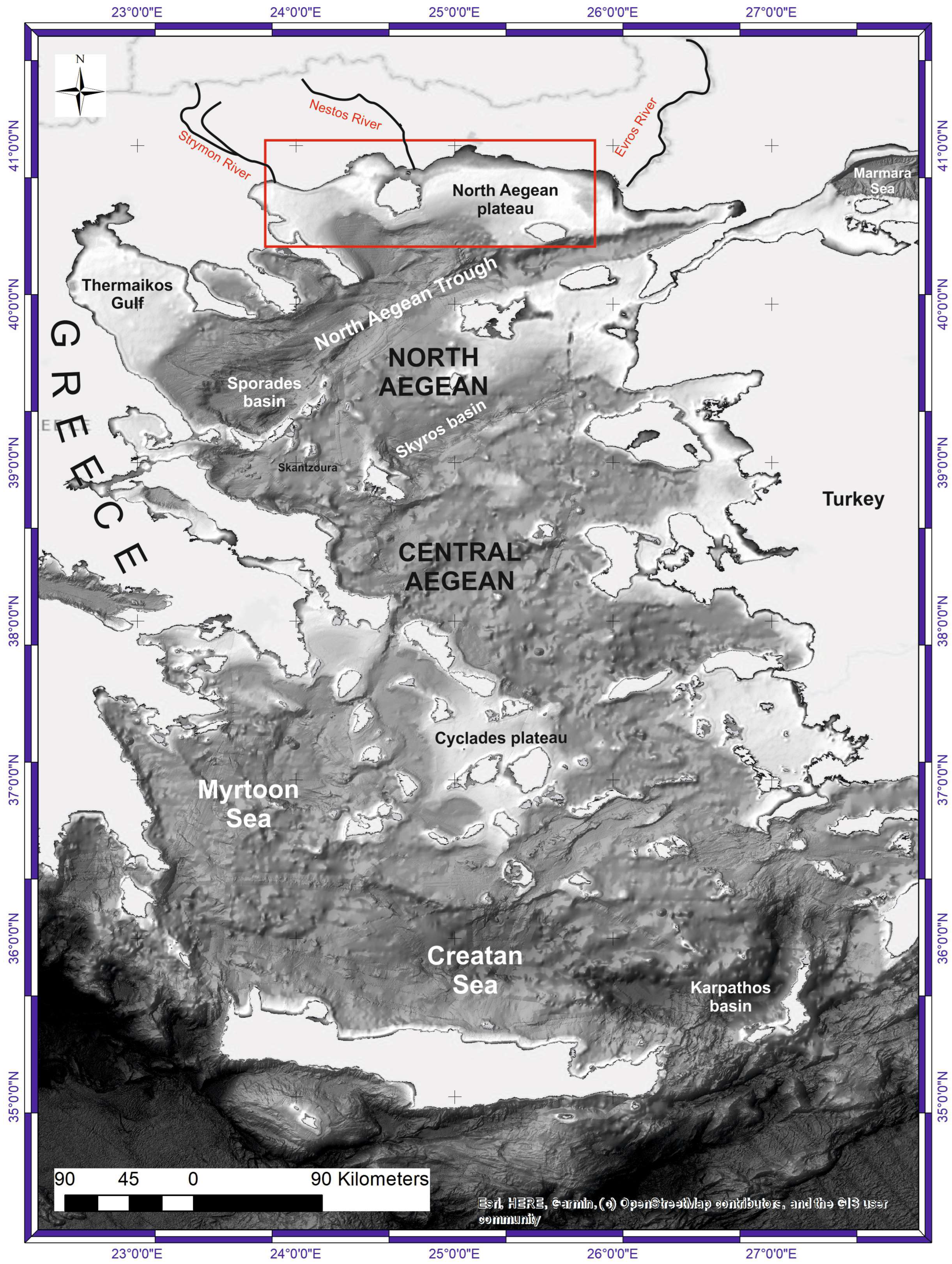
Figure 3.
Ternary diagrams representing sample classification [11].
Figure 3.
Ternary diagrams representing sample classification [11].
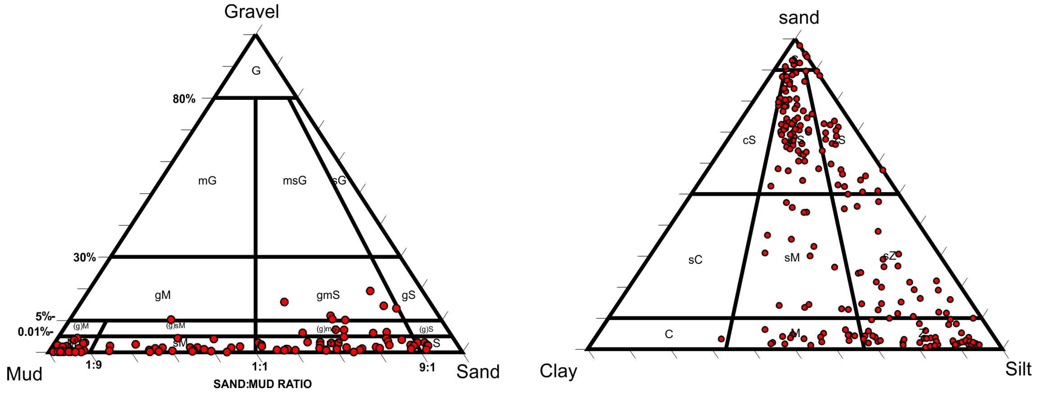
Figure 4.
Spatial distribution of gravel–sand, silt, and clay ((a–c) respectively).
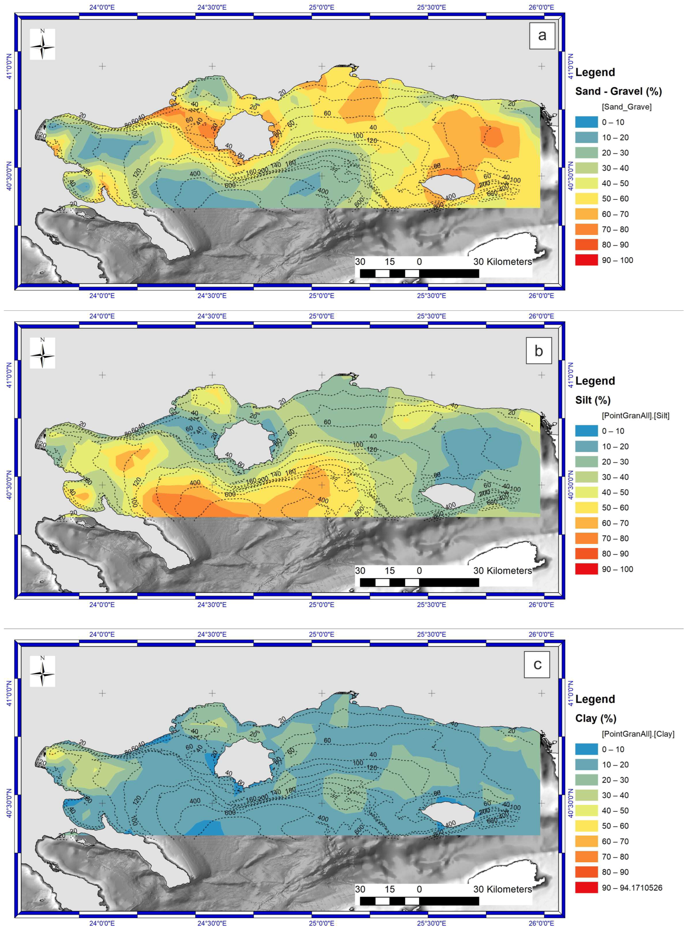
Figure 5.
Statistical parameters (mean, sorting, skewness) spatial distribution ((a–c) respectively).
Figure 5.
Statistical parameters (mean, sorting, skewness) spatial distribution ((a–c) respectively).

Figure 6.
Statistical parameters correlations. The coloring of the various groups of Y-Axis is consistent with the classification presented in Figure 5.
Figure 6.
Statistical parameters correlations. The coloring of the various groups of Y-Axis is consistent with the classification presented in Figure 5.

Figure 7.
(a) Histogram of the average vector length of the 100 randomly distributed datasets. (b) Estimation of vector length L90 for a significance level of 0.1. (c) Estimation of vector length L95 for a significance level of 0.05 and (d) Estimation of vector length L99 for a significance level of 0.01. The red part of the plots corresponds to the critical area for the significance tests.
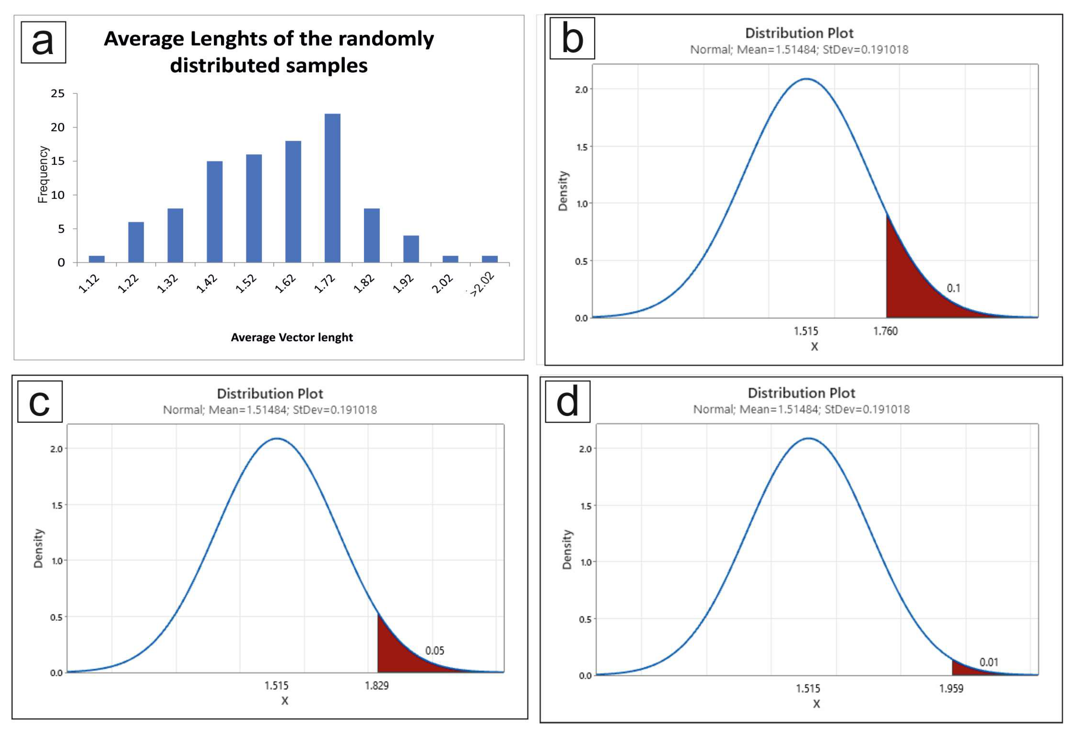
Figure 8.
Net sediment transport pattern across the study area.

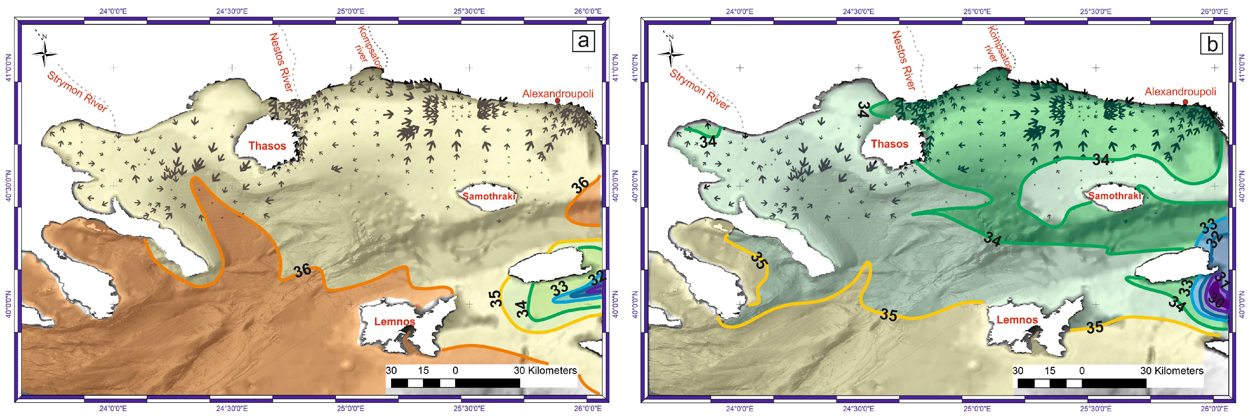
Figure 9.
(a) Generalized water circulation pattern where the flow circulation vectors of the various research are also shown [39,46,47]. (b) Vertical salinity distribution across section AB for winter (modified from [38]). (c) Vertical salinity distribution across section AB for summer (modified from [38]).

Figure 10.
(a) Surface salinity during winter. (b) Surface salinity during summer (modified from [38]).
Figure 10.
(a) Surface salinity during winter. (b) Surface salinity during summer (modified from [38]).
Disclaimer/Publisher’s Note: The statements, opinions and data contained in all publications are solely those of the individual author(s) and contributor(s) and not of MDPI and/or the editor(s). MDPI and/or the editor(s) disclaim responsibility for any injury to people or property resulting from any ideas, methods, instructions or products referred to in the content. |
© 2024 by the authors. Licensee MDPI, Basel, Switzerland. This article is an open access article distributed under the terms and conditions of the Creative Commons Attribution (CC BY) license (https://creativecommons.org/licenses/by/4.0/).
Share and Cite
MDPI and ACS Style
Vakalas, I.; Zananiri, I. Net Transport Patterns of Surficial Marine Sediments in the North Aegean Sea, Greece. J. Mar. Sci. Eng. 2024, 12, 512. https://doi.org/10.3390/jmse12030512
AMA Style
Vakalas I, Zananiri I. Net Transport Patterns of Surficial Marine Sediments in the North Aegean Sea, Greece. Journal of Marine Science and Engineering. 2024; 12(3):512. https://doi.org/10.3390/jmse12030512
Chicago/Turabian StyleVakalas, Ioannis, and Irene Zananiri. 2024. "Net Transport Patterns of Surficial Marine Sediments in the North Aegean Sea, Greece" Journal of Marine Science and Engineering 12, no. 3: 512. https://doi.org/10.3390/jmse12030512
Note that from the first issue of 2016, this journal uses article numbers instead of page numbers. See further details here.