An Adaptive Multimodal Data Vessel Trajectory Prediction Model Based on a Satellite Automatic Identification System and Environmental Data

Abstract

Ship trajectory prediction is essential for ensuring safe route planning and to have advanced warning of the dangers at sea. With the development of deep learning, most of the current research has explored advanced prediction methods based on historical spatio-temporal Automatic Identification System (AIS) data. However, environmental factors such as sea wind and visibility also affect ship navigation in real-world maritime shipping. Therefore, developing reliable models utilizing multimodal data, such as AIS and environmental data, is challenging. In this research, we design an adaptive multimodal vessel trajectory data prediction model (termed AMD) based on satellite AIS and environmental data. The AMD model mainly consists of an AIS-based extraction network, an environmental-based extraction network, and a fusion block. In particular, this work considers multimodal data such as historical spatio-temporal information and environmental factors. Time stamps and distances are correlated with AIS and environmental data, and a multilayer perceptron and gated recurrent unit networks are used to design multimodal feature extraction networks. Finally, the fusion block realizes the fusion output of multimodal features to improve the reliability of the AMD model. Several quantitative and qualitative experiments are conducted using real-world AIS and multimodal environmental datasets. Numerous experimental results prove that prediction performance using multimodal data can ensure satisfactory accuracy and reliability while exhibiting a positive impact on improving maritime transport services.

1. Introduction

The development of world trade has promoted the prosperity of the maritime transportation industry [1]. Therefore, improving maritime safety and ship transport efficiency has been a global focus. Trajectory prediction is important for improving marine traffic safety and transportation efficiency [2,3]. Because prediction technology can predict the behavior of ships in advance, it can realize functions such as the early warning of maritime risks and the planning of safe routes [4]. However, the complexity of the maritime transport environment leaves room for improvement in forecasting technology. For example, there are many ships in ports and densely populated routes; in addition, limited monitoring methods in distant oceans lead to late warnings. Therefore, researchers have become eager to explore more accurate and efficient methods of predicting the trajectory of ships [5,6,7].

The Automatic Identification System (AIS) is utilized for condition monitoring and the condition data management of seagoing vessels [8,9]. It is characterized by its wide coverage and large data volume. AIS data record important information, such as a ship’s position, course, and speed during navigation, which is extremely valuable for studying advanced models in terms of predicting ship trajectories [10]. In particular, satellite-based AIS systems can overcome the limitations of limited distances from land-based base stations and can monitor the status of oceangoing vessels [11]. Therefore, AIS data are frequently utilized to study advanced models for forecasting the trajectory of ships [12].

Existing methods for predicting vessel trajectory fall into three categories: traditional [13,14], machine learning [15,16], and deep learning [17,18,19]. Traditional approaches primarily rely on empirical and mathematical models following specific physical laws [20,21]. However, the application scenarios of traditional methods depend on boundary conditions. Machine learning methods can improve prediction accuracy by creating complex mathematical models to simulate ship movements [22,23]. However, machine learning approaches need to collect a considerable amount of labeled data and the establishment of appropriate rules. Deep learning methods can extract features from large-scale historical ship trajectory data via neural networks and are good at processing nonlinear and high-dimensional data [24,25,26]. However, the complexity of maritime application scenarios and the changing traffic environment leave considerable room for improvement in existing methods.

Notably, during sea travel, ships are affected by various environmental factors such as sea wind, visibility, temperature, etc. These environmental factors influence the speed, direction, and navigation path of the ship. Therefore, relying solely on AIS data is insufficient to achieve highly reliable forecasting methodology. The Maritime Traffic Services System contains AIS data, which are used to monitor ship statuses and maritime environmental data. Therefore, how to build a reliable model for forecasting a ship’s trajectory in a multimodal data environment, such as AIS and environmental data, still needs to be studied.

In this study, we aim to design an adaptive multimodal data vessel trajectory prediction model (termed AMD) based on satellite AIS and environmental data. This model considers the spatio-temporal information and environmental factors that affect ship navigation at sea. The AMD model can make reliable predictions under multimodal data to ensure the safe navigation of vessels at sea. First, a hybrid correlation of AIS and environmental data is performed based on the closest period and shortest distance. Then, a multilayer perceptron (MLP) and gated recurrent unit (GRU) networks are applied to the AIS- and environmental-based extraction networks, respectively, and modal prediction information is integrated to obtain the final prediction result. Finally, a comparison with current existing research validates the effectiveness of the AMD model. Typical tests and ablation experiments also show the effectiveness of the AMD model.

2. Related Works

In intelligent maritime transportation, numerous research efforts have been made to improve prediction performance. These methods can automatically extract features from vast amounts of data and achieve teh high-precision prediction of ship trajectories through complex pattern recognition [27]. More details about these three mentioned approaches are given in the following sections.

2.1. Traditional Methods

Traditional methods typically rely on empirical and mathematical models. These methods forecast ship trajectories through simulation or statistical analysis. Traditional methods mainly include simulation, statistical, knowledge-based, and control theory-based methods. For example, Xu et al. [20] designed a high-precision, long-period oil tanker trajectory prediction algorithm, which applies the density-based spatial clustering of applications with noise (DBSCAN) clustering to process AIS data, as well as extracts a series of key points representing critical navigation modes. They then developed, in turn, a novel path search algorithm to select one part of these key points to generate a predicted trajectory to a fixed target. Zhang et al. [21] presented a big data analysis strategy for proactively reducing baseline risk. The technique groups environmental parameters utilizing k-means and DBSCAN big data clustering methods, as well as principal component analysis, and it then predicts chosen ship movement dynamics employing multi-output Gaussian process regression. Xiao et al. [28] introduced a novel model that integrates motion modeling and filtering processes. Srivastava et al. [14] presented a lightweight, short-term forecast model based on linear stationary models for ship trajectory prediction and real-time anomaly detection. They integrated the best-fitting auto-regressive integrated moving average (ARIMA) model with window generator models of different sizes and visualizations for recursive real-time predictions. However, these methods often have data quality and model complexity limitations, thus making it difficult to make highly accurate predictions. For example, simulation methods may have difficulty dealing with significant time interval uncertainties. Statistical methods are based on similarity searches and Bayesian inference. Knowledge-based methods require the extraction, storage, and retrieval of knowledge. These limitations point to the need for more advanced prediction techniques.

2.2. Machine Learning Methods

A growing number of studies are focusing on using machine learning methods to ship trajectories. Zhang et al. [29] designed a position prediction approach to increase ship position forecast accuracy in ship traffic engineering by employing the k-nearest neighbors (KNN) algorithm. Sedagha et al. [22] presented a system framework for online maritime traffic monitoring aimed at the real-time tracking of vessels on waterways and the prediction of their subsequent positions. Through employing a decomposition reconstruction process and adaptive segmented error correction, Wei et al. [30] developed a multi-objective heterogeneous integration approach for predicting ship motion. Xiao et al. [31] designed a machine learning model employing physical information to build a gray box model (GBM) to predict the speed of ships crossing the ocean. Dong et al. [23] introduced a new mathematical data integration prediction (MDIP) model for predicting the maneuvering movement of ships. The MDIP model, proposed using mathematical data integration, exhibits greater generalization ability and opens up new ways for predicting the maneuvering movement of ships. However, machine learning methods require extensive data labeling and exhibit a weak learning ability for the dynamic characteristics of ships. Therefore, the training and prediction of machine learning models still face numerous challenges.

2.3. Deep Learning Methods

Deep learning methods are reasonable at utilizing neural networks to extract high-dimensional features from large amounts of data and have been widely employed. Wu et al. [32] designed a combined convolutional long short-term memory (LSTM) and sequence-to-sequence (Seq2Seq) model for improved accuracy. Chen et al. [24] designed a new framework to obtain and predict ship trajectories more accurately using the bidirectional LSTM (BiLSTM) model. Zhao et al. [26] designed a model for predicting ship trajectories using a graph attention network (GAT) and the LSTM model. Guo et al. [33] proposed a multimodal-data-based approach for predicting ship trajectories by incorporating additional hidden states to define complex modes independently. A context-driven, data-driven framework for predicting ship trajectories was presented by Mehri et al. [34]. This framework first enriched the contextual information of a trajectory, including the evaluation methods for annotating a trajectory, and then applied feature selection techniques to solve high-dimensional problems. Finally, selected factors were used in the context-aware LSTM network. However, current deep learning methods still face numerous challenges. For example, they have difficulty effectively fitting complex environmental changes and uncertainty factors. In this study, we investigate how to develop efficient methods for predicting ship trajectories under complex environmental factors.

3. Preliminaries

3.1. Problem Definition

A multimodal dataset containing AIS and environmental data can be defined as time-ordered tuple sequences $S=\{T,P,E\}$ containing N samples. The sequence contains a list of time points $T=\{t_1,\dots ,t_N\},t_1<\dots <t_N$, a discrete space–time sequence $P=\{p_1,\dots ,p_N\},p_1<\dots <p_N$, and a discrete environment sequence $E=\{e_1,\dots ,e_N\},$$e_1<\dots <e_N$.

The problem of neural network-based trajectory prediction is the difficulty in learning spatio-temporal mapping from a multimodal dataset that can predict future motion locations based on previously observed features. We adopted a sliding window to rearrange S into a new data representation. The input sequence $X_g\triangleq {\left\{x_i\right\}}_{i=1}^g={\left\{t_i\right\}}_{i=1}^g\bigcup {\left\{p_i\right\}}_{i=1}^g\bigcup {\left\{e_i\right\}}_{i=1}^g\in {\mathbb{R}}^{d\times g}$ is represented as a sequence with input length g, the output sequence ${\mathrm{Y}}_l\triangleq {\left\{y_i\right\}}_{i=1}^l={\left\{p_i\right\}}_{i=1}^l\in {\mathbb{R}}^{d\times l}$ is defined as a sequence with output length l, and d represents the data dimension.

3.2. Multilayer Perceptron Network

The MLP network comprises input, hidden, and output layers [35,36]. We define the observation sequence ${\mathrm{X}}_g^{\mathrm{ais}}={\left\{x_t^{\mathrm{ais}}\right\}}_{t=1}^g$ in the AIS dataset to represent a trajectory spatio-temporal sequence of length g. The internal hidden state is updated as the elements in the input sequence are read sequentially:

$$h_j={\sigma }_j(h_{j-1}{w}_j+b_j;\theta ).$$

(1)

An activation function with $\theta$-learnable parameters is represented by ${\sigma }_j$. In the j-th hidden layer, $b_j$ represents bias, while $w_j$ represents weight. Finally, the output layer receives the hidden layer state $h_j$ as an input to make sequential predictions.

3.3. GRU Network

Figure 1a shows that the GRU network is less complex than LSTM. This difference is because the GRU network uses fewer gates and does not have a separate internal memory. The GRU relies entirely on hidden states as its memory, thus resulting in a simpler architecture. Therefore—compared to LSTM (as shown in Figure 1b), which has a greater number of gates and states—the GRU has fewer parameters and may have less computational complexity. The GRU algorithm allows for faster convergence and internal weight updates [37]. The gating vector can determine whether the information in the long-term sequence is not cleared or removed over time.

We define the observation sequence ${\mathrm{X}}_g^{\mathrm{env}}={\left\{x_t^{\mathrm{env}}\right\}}_{t=1}^g$ in the environmental dataset to represent an ecological mode sequence of length g. The GRU algorithm reads the elements in the sequence one by one and updates the internal hidden state. Specifically, the refresh rate at time t is calculated using the following formula:

$$z_t=\sigma (W_z{x}_t^{\mathrm{env}}+U_z{h}_{t-1}+b_z),$$

(2)

where the input vector at time step t, denoted as $x_t^{extenv}$, is the t-th element of the environmental modal input sequence $ext{X}_g^{extenv}$, which experiences a linear transformation. In addition, $h_{t-1}$ saves the previous time step $t-$1, and $W_z$ and $U_z$ are weight matrices.

Update gates determine the amount of past information that is needed to propagate into the future. The following expression calculates the reset gate:

$$r_t=\sigma (W_r{x}_t^{\mathrm{env}}+U_r{h}_{t-1}+b_r).$$

(3)

The reset gate stores past relevant information through the following formula:

$$h_t^{\prime }=tanh(W_h{x}_t^{\mathrm{env}}+r_t\odot U_h{h}_{t-1}+b_h).$$

(4)

The input $x_t^{\mathrm{env}}$ and the previous statement $h_{t-1}$ change linearly through the weight matrices $W_h$ and $U_h$; then, the corresponding element product $r_t$ and hadamard product $U_h{h}_{t-1}$ are calculated. In addition, $h_t$ is calculated using the following formula:

$$h_t=(1-z_t)\odot h_{t-1}+z_t\odot h_t^{\prime },$$

(5)

where $z_t$ and $h_{t-1}$ denote the information retained between time steps.

4. Adaptive Multimodal Data Method

4.1. Overview Architecture

To address the trajectory prediction problem described in the previous section, we propose a new AMD model. Our model is designed to map AIS and environmental multimodal data input sequences to the output sequences of specified lengths. In a given time step s, our model aims to learn the following prediction distribution:

$$p(y_1,\dots ,y_l|x_1,\dots ,x_g),$$

(6)

which represents the $Y_l$ probability that g multimodal observation data in a given input sequence $X_g$ map to the l target trajectory sequences in the future. The neural network model can directly sample the target sequence once the predictive distribution has been learned.

The task of the proposed AMD model is essentially a regression problem. The purpose is to train the adaptive multimodal data neural network-based model $M_{g,l}$ using AIS $X_g^{\mathrm{ais}}$ and environmental $X_g^{\mathrm{env}}$ data. An output sequence $Y_l$ of length l is generated, thereby maximizing the conditional probability Equation (6), that is

$$Y_l=M_{g,l}(X_g^{\mathrm{ais}},X_g^{\mathrm{env}})=argmax{Y}_p\left(Y_l\right|X_g^{\mathrm{ais}},X_g^{\mathrm{env}}),$$

(7)

where the parameterized function $M_{g,l}(X_g^{\mathrm{ais}},X_g^{\mathrm{env}};\theta )$ can be trained from a given multimodal dataset to find the parameter set $\hat{\theta }$ in the training samples nearest to the mapping function in Equation (7), thereby minimizing the following task-relevant error measure L:

$$\hat{\theta }=arg{min}_{\theta }\frac{1}{N}{\sum }_{i=1}^{N}L(M_{g,l}(X_g^{\mathrm{ais}},X_g^{\mathrm{env}}),Y_l^i),$$

(8)

where N represents the overall sample count, and $(X_g^{\mathrm{ais}},X_g^{\mathrm{env}})$ and $Y_l^i$ denote the input and target sequences.

Figure 2 shows that the AMD model mainly contains an AIS-based extraction network, a weather-based extraction network, and a fusion block. First, the observation sequence $X_g^{\mathrm{ais}}$ is read based on the AIS extraction network, and the temporary prediction value ${\mathrm{Y}}_l^{\mathrm{ais}}$ is obtained through neural network training. Then, the environment observation sequence $X_g^{\mathrm{env}}$ is read based on the environment extraction network, and the temporary prediction value ${\mathrm{Y}}_l^{\mathrm{env}}$ is obtained through neural network learning. The FC is the fully connected layer, which is used to transform the matrix learned via the modal data feature extraction network according to the target sequence dimension. Finally, the fusion block fuses the predicted values ${\mathrm{Y}}_l^{\mathrm{ais}}$ and ${\mathrm{Y}}_l^{\mathrm{env}}$ to generate the ${\mathrm{Y}}_l$ of the final future trajectory.

We learn the mapping relationship $M_{g,l}$ in Equation (9) through AIS- and environmental-based extraction networks. The initial calculation functions are given in the following formulas:

$${\mathrm{Y}}_l^{\mathrm{ais}}=M_{\mathrm{ais}}({\mathrm{X}}_g^{\mathrm{ais}};{\theta }_{\mathrm{ais}}),$$

(9)

$${\mathrm{Y}}_l^{\mathrm{env}}=M_{\mathrm{env}}({\mathrm{X}}_g^{\mathrm{env}};{\theta }_{\mathrm{env}}).$$

(10)

A neural network with parameters ${\theta }_{\mathrm{ais}}$ and ${\theta }_{\mathrm{env}}$ can be described using Equations (9) and (10). A mapping ${\theta }_{\mathrm{ais}}$ is defined between the input sequence $X_g^{\mathrm{ais}}$ and internal expressions ${\mathrm{Y}}_l^{\mathrm{ais}}={\left\{h_t^{\mathrm{ais}}\right\}}_{t=1}^g$, such that $h_t^{\mathrm{ais}}\in {\mathbb{R}}^q$ is the output of the MLP’s hidden state. ${\theta }_{\mathrm{env}}$ maps the input sequence $X_g^{\mathrm{env}}$ to the internal expression sequence ${\mathrm{Y}}_l^{\mathrm{env}}={\left\{h_t^{\mathrm{env}}\right\}}_{t=1}^g$, such that $h_t^{\mathrm{env}}\in {\mathbb{R}}^q$ is the fully connected layer output of the hidden state connection GRU.

Finally, through the fusion block pairs ${\mathrm{Y}}_l^{\mathrm{ais}}$ and ${\mathrm{Y}}_l^{\mathrm{env}}$, the mapping relationship $M_{g,l}$ in Equation (7) is fused and learned, and the following output sequence of length l is finally generated:

$$Y_l=F_{2l}([Y_l^{\mathrm{ais}},Y_l^{\mathrm{env}}];{\theta }_F),$$

(11)

where Equation (11) is a neural network with ${\theta }_F$ as a parameter, which maps the input intermediate prediction value to a series of internal representations ${\mathrm{Y}}_h={\left\{h_t^{\mathrm{fused}}\right\}}_{t=1}^{2l}$, such that $h_t^{\mathrm{fused}}\in {\mathbb{R}}^q$ is the output after fusion and addition.

In our study, the AIS-based extraction and prediction network utilizes the MLP network, and the environmental-based extraction and prediction network employs the GRU network. The following subsections will provide more details about AIS- and environmental-based extraction networks, as well as fusion blocks.

4.2. AIS-Based Extraction Network

The observation sequence in the AIS data is captured via the neural network input layer based on the AIS extraction network. Afterward, the hidden layer learns the weights and parameters, and the fully connected layer outputs predictions. We employ Equation (9) to map ${\mathrm{X}}_g^{\mathrm{ais}}$ to the output, that is, the hidden sequence ${\mathrm{H}}_g^{\mathrm{ais}}\triangleq {\left\{h_t^{\mathrm{ais}}\right\}}_{t=1}^g,h_t^{\mathrm{ais}}\in {\mathbb{R}}^q$, and this is iterated through the following neural network function:

$$h_t^{\mathrm{ais}}=\mathrm{MLP}(x_t^{\mathrm{ais}},h_{t-1}^{\mathrm{ais}};{\theta }_{\mathrm{ais}}).$$

(12)

In Equation (9), ${\mathrm{Y}}_l^{\mathrm{ais}}$ is a sequence of length l obtained via the hidden layer output vector $\{h_1^{\mathrm{ais}},\dots ,h_g^{\mathrm{ais}}\}$ after another connection operation. The AIS-based extraction network encodes the spatio-temporal information from each element $h_t^{\mathrm{ais}}\in {\mathbb{R}}^q$.

4.3. Environmental-Based Extraction Network

The GRU neural network uses a environmental-based extraction network to capture the observation sequence in the environmental data. Afterward, the hidden layer learns the weights and parameters, and the fully connected layer outputs the predictions. We employ the GRU network in Equation (10) to map the $X_g^{\mathrm{env}}$ to the output, that is, the hidden sequence ${\mathrm{H}}_g^{\mathrm{env}}\triangleq {\left\{h_t^{\mathrm{env}}\right\}}_{t=1}^g,h_t^{env}\in {\mathbb{R}}^q$, and this is iterated through the following neural network function:

$$h_t^{\mathrm{env}}=\mathrm{GRU}(x_t^{\mathrm{env}},h_{t-1}^{\mathrm{env}};{\theta }_{\mathrm{env}}).$$

(13)

In Equation (10), ${\mathrm{Y}}_l^{\mathrm{env}}$ is a sequence of length l obtained after performing another connection operation on the hidden layer output vector $\{h_1^{\mathrm{env}},\dots ,h_g^{\mathrm{env}}\}$. Each element $h_t^{\mathrm{envs}}\in {\mathbb{R}}^q$ encodes the environmental modal information input from the t-th component of the sequence to the environmental-based extraction network.

4.4. Fusion Block

The fusion block of Equation (11) aims to generate future trajectories given the temporarily predicted values ${\mathrm{Y}}_l^{\mathrm{ais}}$ and ${\mathrm{Y}}_l^{\mathrm{env}}$. Mathematically, the fusion prediction block decomposes the fusion probability into ordered conditions to calculate the conditional probability given the temporary prediction value. Given the prediction sequences based on AIS and environment extraction networks, observations and future sequences are assumed to be conditionally independent as follows:

$$p\left(y_j\right|y_1,\dots ,y_{j-1})=F([Y_l^{\mathrm{ais}},Y_l^{\mathrm{env}}],u_j;{\theta }_F),$$

(14)

where the future trajectory $y_j$ is calculated via F given the temporary prediction values ${\mathrm{Y}}_l^{\mathrm{ais}}$ and ${\mathrm{Y}}_l^{\mathrm{env}}$, the observation sequence for time step j, and $u_j$ in the fusion prediction block.

4.5. Data Preprocessing

We elaborated on the data preprocessing process with regard to the association between AIS and the environmental data, as well as with respect to the processing of training data.

4.5.1. Correlating AIS and Environmental Data

This study adopted real-world AIS and environmental data. Each row in the AIS dataset records the ship’s spatio-temporal message, including the timestamp ($time$), the maritime mobile service identity ($MMSI$), longitude ($lon$), latitude ($lat$), course over ground ($cog$), and speed over ground ($sog$). Each row in the environmental dataset records local weather data, including timestamp ($time$), longitude ($lon$), latitude ($lat$), wind ($win$), visibility ($vis$), and temperature ($temp$). The original AIS data do not contain environmental factors and need to be effectively correlated. Therefore, we utilized the closest and shortest distance methods to correlate the AIS and environmental information.

Firstly, for each AIS data point, the closest environmental message cluster was selected from the environmental dataset based on the timestamp field.

Secondly, the environmental data nearest to the AIS data were selected from the filtered environmental message clusters.

Finally, the filtered environmental data were combined with the AIS data to form new multimodal original data containing both AIS and environmental data.

The above steps were repeated to form a new multimodal AIS and environmental dataset.

4.5.2. Dataset Normalization

To ensure the quality of data utilization, we preprocessed the correlated multimodal dataset. Normalization can eliminate the differences in data across different dimensions in the original dataset while preserving data characteristics as much as possible. The min–max normalization method was applied to normalize the multimodal datasets, as shown in the following formula:

$$X^{*}=\frac{X-minx}{maxx-minx},$$

(15)

where X denotes the original data, $\max x$ denotes the maximum value, and $\min x$ and $X^{*}$ are the minimum and normalized data, respectively.

To avoid distorting the obtained model due to any changes in the regional extent, when normalizing the longitudinal and latitudinal values, we set the longitudinal $max{x}_{lon}$ = 180 and $min{x}_{lon}$ = −180, as well as the latitudinal $max{x}_{lat}$ = 90 and $min{x}_{lat}$ = 0. We did not utilize the maximum and minimum longitudinal and latitudinal values within the data of a given area.

Meanwhile, to obtain multiple continuous space–time sub-trajectory sequence data for each ship, a window sliding method based on timestamps was applied to segment the normalized dataset. The length of the observed sequence for each sub-trajectory is g, and the size of the predicted sequence trajectories is l. The proposed AMD model can set a reasonable data input and output length according to the task requirements.

4.6. Implementation Details

This subsection mainly introduces the detailed configuration of the AMD model. Our model was implemented on the Python 3.6 platform, and all experiments were performed on a PC equipped with an Intel Xeon(R) E5-2650L v3 @ 1.80 GHz CPU with 32 GB of RAM. Multivariate input sequences were first transferred into 64 units for analysis using MLP and GRU networks, and this was followed by a step-by-step learning of the output sequences. Using Adam’s algorithm, the batch size was 64 and the number of epochs was 300. The detailed configuration is shown in

Table 1. Detailed configuration information of the training process.

Name	Value
Learning rate	0.001
Batches	64
Optimizer	Adam
Epochs	300
Loss function	MSE
Activation	tanh

. In addition, before training the network, the dataset was split into 70% training and 30% testing sets.

5. Results and Analysis

5.1. Datasets and Evaluation Metrics

This study mainly used AIS and environmental datasets from the geographical area of the Australian and Argentinian oceans. The AIS dataset was obtained from the China Maritime Safety Administration, and the environmental dataset was obtained from the National Centers for Environmental Information Data. Specifically, we selected the data from 1 April to 30 April 2020 to verify this research method. As shown in Figure 3, we chose the marine around Australia and southern Argentina. The detailed latitudinal and longitudinal range of the selected sea areas is shown in

Table 2. Latitude and longitude area.

	Longitude		Latitude
	Min.	Max.	Min.	Max.
Australia	105.65	178.85	−54.92	−6.56
Argentina	−100.36	−30.46	−66.91	−32.23

. We verified the effectiveness of the AMD model using the two datasets. After the AMD model was trained on one of the sea areas, it was not directly transferred to the other sea area for direct use. Data preprocessing was performed for AIS and environmental data using the preprocessing method. The results before and after processing are shown in

Table 3. Preprocessing entries for AIS and environmental datasets.

Datasets	AIS Data (Rows)			Environmental Data (Rows)
	Raw Data Entries	Preprocessed Data Entries	Ships	Raw Data Entries	Preprocessed Data Entries
Australia	795,132	314,865	176	1,168,140	380,066
Argentina	1,485,687	631,027	227	872,199	217,859

.

The AIS dataset of the Australian oceans has three characteristics: (1) in some areas, navigation is intensive, and there are scenarios with high maritime traffic complexity; (2) there are intensive ship activities at sea, and the tracks in the Australian marine area are dense, as shown in Figure 3; and (3) many types of ships exist, as described in the following Section 5.3.2, and the dataset includes eight types of ships, with each ship’s primary business at sea being different. Given these marine areas with dense routes, various ship types, and high complexity, there is an urgent need to improve maritime traffic safety and rationally plan routes for maritime ship navigation to avoid ship collisions.

This study mainly used $RMSE$, $MAPE$, and $MAE$ metrics to evaluate the usefulness of the AMD model. An error between the observed and predicted value was calculated to measure the quality of the vessel trajectory prediction task. Specifically, the aforementioned metric formulas were computed as follows:

$$RMSE=\sqrt{\frac{1}{N}{\sum }_{i=1}^N\left[{\left({\widehat{lat}}_i-la{t}_i\right)}^2+{\left({\widehat{lon}}_i-lo{n}_i\right)}^2\right]},$$

(16)

$$MAPE=\frac{100\%}{N}{\sum }_{i=1}^N\left(\left|\frac{{\widehat{lat}}_i-la{t}_i}{la{t}_i}\right|+\left|\frac{{\widehat{lon}}_i-lo{n}_i}{lo{n}_i}\right|\right),$$

(17)

where $lat$ and $lon$ are the observed values, and $\widehat{lat}$ and $\widehat{lon}$ are the predicted values. N denotes the total samples. A smaller error value means a better prediction.

Furthermore, we computed the distance between the predicted and observed values employing the haversine formula. The half-positive vector distance of any two trajectory points, such as $p_1$ and $p_2$, is calculated as follows:

$$di{s}_H=2Rarcsin\sqrt{{sin}^2\left(\frac{la{t}_2-la{t}_1}{2}\right)+coslo{n}_{1}coslo{n}_2{sin}^2\left(\frac{lo{n}_2-lo{n}_1}{2}\right)},$$

(18)

where R denotes the Earth’s radius. Using nautical miles ($nmi$) as the distance measurement unit, we define the mean square error $MAE$ for N sample points to evaluate the AMD model performance better:

$$MAE=\frac{1}{N}{\sum }_{i=1}^{N}di{s}_H\left({\hat{y}}_i,y_i\right).$$

(19)

A predicted trajectory value is denoted by ${\hat{y}}_i$, while a measured (ground truth) trajectory value is denoted by $y_i$.

5.2. Quantitative Analysis

For a detailed comparison, we compared the AMD model against the current work on vessel trajectory prediction. We used the LSTM [38], GRU [39], ANN [40], BLSTM [41], EncDec [42], MPLSTM [43], and ST-Seq2seq [44] models as the baseline models. In particular, LSTM and GRU are variant models of RNN networks, and several other models are effective trajectory prediction methods that were built using neural networks. Each model sets its learning rate for training according to the baseline model. The detailed configuration is shown in

Table 4. Detail parameter table for baseline models.

Model	Learning Rate	Input Layer	Batch Size	Activation
LSTM [38]	0.001	18	64	tanh
GRU [39]	0.001	18	64	tanh
ANN [40]	0.001	18	64	tanh
BLSTM [41]	0.005	18	5000	tanh
EncDec [42]	0.0001	18	200	tanh
MPLSTM [43]	0.001	18	64	tanh
ST-Seq2seq [44]	0.001	18	64	tanh

. The models were trained on the training set to obtain trainable models, and these were then evaluated on the test set.

Our experimental results were based on the Australian and Argentina datasets.

Table 5. Comparison of the prediction results of the various models under Australian and Argentina datasets.

Baseline Models	Australia Datasets			Argentina Datasets
	RMSE (${\mathbf{10}}^{-\mathbf{3}}$)	MAPE (${\mathbf{10}}^{-\mathbf{3}}$)	MAE ($\mathit{nmi}$)	RMSE (${\mathbf{10}}^{-\mathbf{3}}$)	MAPE (${\mathbf{10}}^{-\mathbf{3}}$)	MAE ($\mathit{nmi}$)
LSTM [38]	0.493	1.011	3.648	0.262	0.535	1.082
GRU [39]	0.362	0.454	4.005	0.343	0.826	1.663
ANN [40]	0.782	1.216	7.871	0.476	1.743	3.526
BLSTM [41]	1.043	1.710	6.776	0.775	2.418	5.656
EncDec [42]	0.913	1.847	6.924	0.434	1.273	2.687
MPLSTM [43]	0.397	0.913	2.835	0.386	0.695	2.073
ST-Seq2seq [44]	121.686	200.164	1450.614	52.652	200.713	450.236
Our model	0.161	0.195	0.843	0.254	0.244	0.624

shows that the AMD model was the most effective on various evaluation indicators. Specifically, in terms of $RMSE$ and $MAPE$ metrics, the results of various models in the Australian dataset showed that our model exhibited improvements of at least 55.4% and 57.09%, respectively. These results proved that using AMD modal information with various neural networks to adapt to multimodal AIS and environmental data has obvious advantages in improving vessel trajectory prediction capabilities.

Moreover, when contrasted against the seven comparison models, the AMD model improved, on average, by 75.44% in terms of the $RMSE$ evaluation metric on the Australian dataset. Compared to the benchmark models, the $RMSE$ of the AMD model improved by 45.49% on the Argentina dataset. It is worth noting that the prediction results of the ST-Seq2seq baseline model deviated from other models by more than 100 times. This showed that the ST-Seq2seq model does not perform well on our ocean dataset, which is closely related to the ST-Seq2seq model design goals and dataset.

$MAE$ measures the error between a model’s predicted and actual values. As shown in Table 5, the AMD model improved by an average of 84.39% and 74.66% compared to the baseline comparison model on the Australian and Argentina datasets, respectively. We selected the ship’s trajectory data ($MMSI$ = 636,092,810) on the Australian dataset and the ship’s ($MMSI$ = 740,349,000) on the Argentina dataset to draw a schematic trajectory diagram. We set the length of the observation sequence and the target prediction sequence to 9.

To explicitly show the effectiveness of the AMD model, we selected a period of historical trajectory data in the dataset as the test data to draw a trajectory display chart. We defined the known trajectory in the input prediction model as the ‘observation’ trajectories and the actual trajectory of the target predicted trajectory segment as the ‘truth’ trajectories. Among them, the ‘observation’ trajectories are also the same starting point sequence of the different prediction models. As shown in Figure 4, across different datasets, AMD’s prediction was closest to the true trajectory. However, the predicted trajectories of the other models significantly deviated by several nautical miles. This trajectory diagram is consistent with the experimental results. In summary, our AMD model achieved satisfactory performance in vessel trajectory prediction.

5.3. Qualitative Analysis

5.3.1. Comparison with Sub-Extraction Models

As mentioned earlier, the AMD model was based on MLP and GRU networks. To verify the efficacy of the AMD model, we compared it to those from the sub-extraction models constructed from MLP and GRU. AIS and environmental datasets were directly associated with training the sub-model. That is, the input dimension and input step were 10 and 2, respectively.

The AMD model exhibited better prediction across various evaluation indicators when compared to the sub-model, as shown in

Table 6. Comparison of the AMD model with the sub-extraction model.

Datasets	Models	RMSE (${10}^{-4}$)	MAPE (${10}^{-4}$)
Australia dataset	MLP sub-model	8.96	8.32
	GRU sub-model	4.59	7.05
	Our	1.61	1.95
Argentina dataset	MLP sub-model	3.52	8.66
	GRU sub-model	3.22	5.83
	Our	2.54	2.44

. Through comparing the predicted value and the actual value evaluation index $MAE$, Figure 5 shows that our proposed model performed best on the two datasets used for evaluation. This experimental result proved that simply utilizing a single neural network to train mixed AIS and environmental data cannot achieve prediction results with good accuracy.

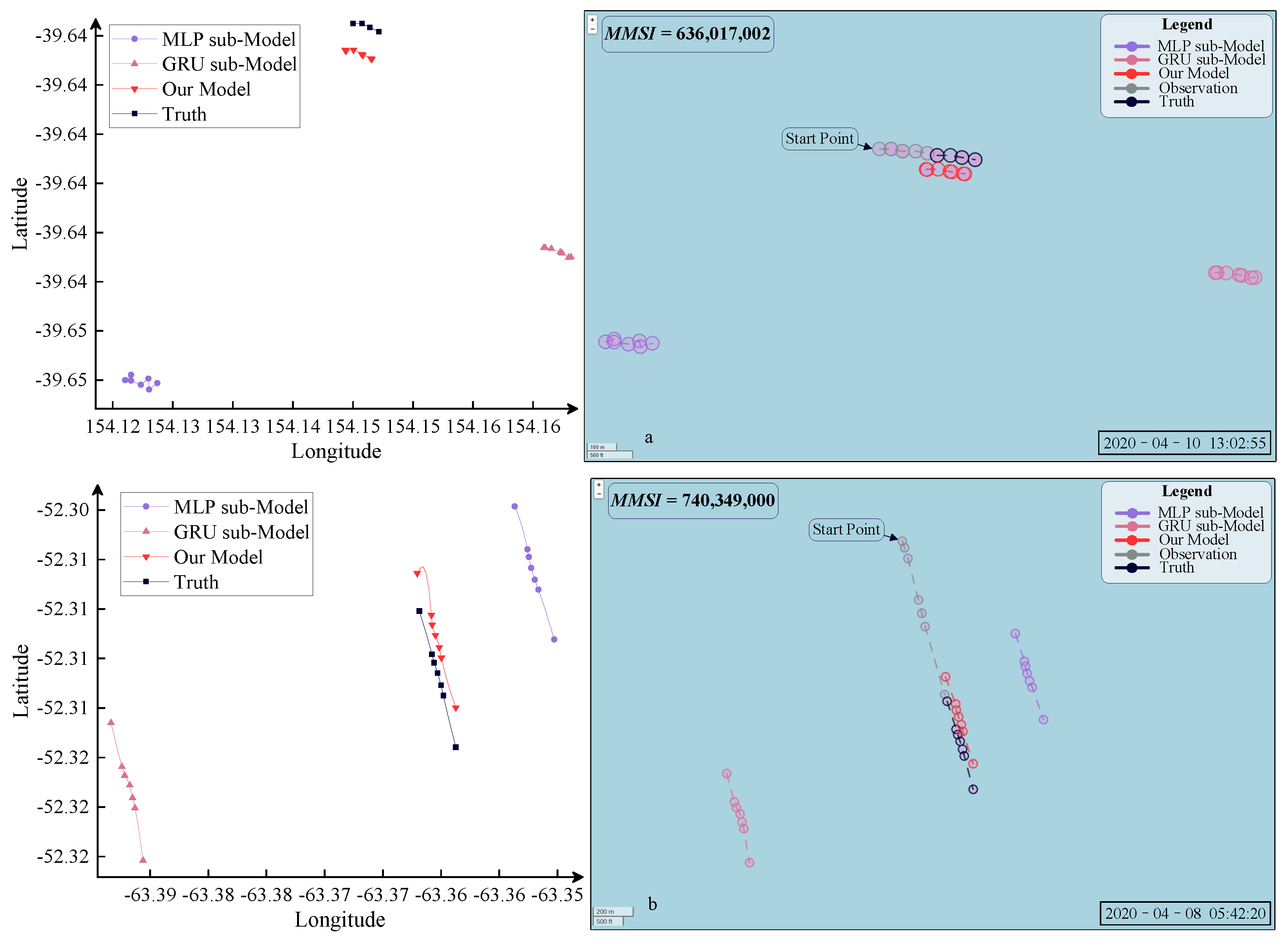
We extracted the ship’s trajectory data ($MMSI$ = 636,017,002) from the Australian dataset and the ship’s trajectory data ($MMSI$ = 740,349,000) from the Argentina dataset, and we also drew a schematic diagram of the AMD model and sub-model trajectory. The AMD model predicted the trajectory more accurately than the single model, as shown in Figure 6. Therefore, AIS-based and environmental-based multimodal data fusion prediction can improve the reliability of ship trajectory prediction.

5.3.2. Comparison of Different Types of Ships

There are many types of ships at sea, and the navigation characteristics of each ship are different. For example, obvious patterns can be seen in some ship tracks, while others are scattered due to a lack of regularity. The results of the prediction model differ depending on the vessel type. As shown in

Table 7. The different ship type numbers that correspond to ship types.

Types Number	Type Names
20	Wing in ground (WIG)
30	Fishing
40	High speed craft (HSC)
50	Pilot vessel
60	Passenger
70	Cargo
80	Tanker
90	Other type

, there are eight types of ship data in the Australian dataset.

The data of these eight ship types were separated from the dataset; then, our trained AMD model was used to predict the experimental results for different ship type datasets. As shown in Figure 7, under the $RMSE$ and $MAPE$ evaluation metrics, the ship types of 20 (wing-effect craft) and 40 (high-speed craft) had the best prediction results. This may be related to the satellite AIS receivers exceeding the distance limit. In general, land-based AIS receivers cannot effectively collect ship data due to distance limitations, but satellites can overcome this limitation.

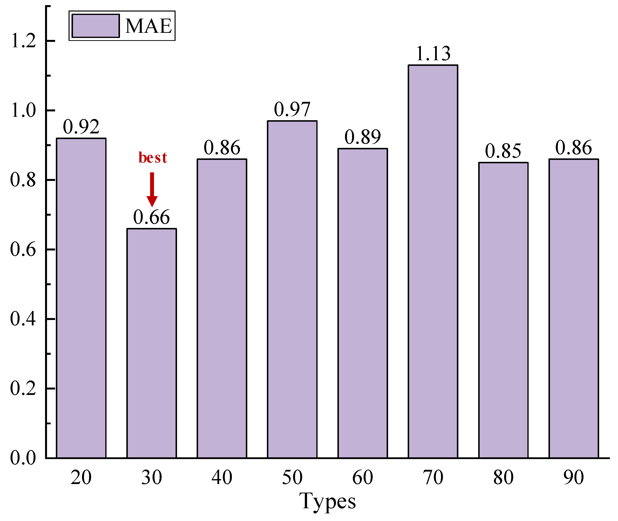
As shown in Figure 8, when the ship type = 30 (fishing boat), the error of the AMD model is the smallest. This is because fishing boats often operate in designated activity areas, and the AMD model can learn certain regular vessel trajectory characteristics more easily. Notably, the scientific magnitudes of the $RMSE$ and $MAPE$ evaluation indicators were very small, and the errors between the different types of ships were not very different. Moreover, the $MAE$ evaluation index showed that the prediction results of the various types of boats hardly differed. The AMD model predicted similar results for different types of ships, thereby proving that the AMD model can be well adapted for the prediction of ship trajectories.

5.4. Ablation Experiments Used to Verify the AMD Model’s Superiority

5.4.1. Comparison of the Prediction Results of Different Network Structures

In contrast to using AIS datasets to study the methods for predicting ship trajectories, this study also combined environmental modal data. Both AIS data and environmental data exhibited temporal sequence features. We compared the AIS and environmental data learning networks with typical networks to verify the superiority of the multimodal datasets. As shown in

Table 8. The five variant models composed of typical network structures.

	Variant 1	Variant 2	Variant 3	Variant 4	Variant 5
AIS ex-net	gru	lstm	gru	gru	bigru
Environmental ex-net	gru	lstm	bigru	lstm	mlp
Variant model	dgru	dlstm	grubigru	grulstm	bigrumlp

, five variant models were set up for comparison. The data training process and evaluation indicators were consistent with the proposed AMD method.

Figure 9 shows the experimental results of the variant model on the two datasets. The multimodal merger prediction network consisting of MLP and GRU networks performed best. The reason for this was that the ship navigation data in the two sea areas were dense, and the spatio-temporal information data were sufficient; thus, the AIS data have linear entity characteristics. Therefore, utilizing MLP works best in the AIS data extraction network. However, the space–time information itself was not directly related. We employed the nearest time and shortest distance techniques to combine the two types of modal data, thereby establishing a correlation between the environmental and spatio-temporal information. It had a weakly nonlinear time series data characteristic. Thus, the GRU network was the best in terms of environmental data extraction.

5.4.2. Comparison of the Prediction Results under Various Combinations of Environmental Factors

This study explicitly considered three environmental factors: wind (including wind speed and direction), visibility, and air temperature. This section details the series of experiments that were set up to verify whether considering sufficient environmental factors is necessary to improve the AMD model’s reliability. Specifically, six comparison experiment groups were created using the control variable method. The AIS data input dimension information remained unchanged and the environmental data factor input type changed. That is, the environmental dataset contains only win factors; only $vis$ factors; only $temp$ factors; $win$ and $vis$ factors; $win$ and $temp$ factors; and $temp$ and $vis$ factors. The AMD method we designed was trained on these six comparison datasets to obtain a model; then, the prediction results were obtained when the model was applied to the test dataset.

Table 9. Prediction results of the AMD model under different combinations of environmental factors (Australian dataset).

	win	vis	temp	win and vis	win and temp	temp and vis	win, vis and temp
RMSE (${10}^{-4}$)	4.61	3.72	6.66	5.13	4.82	5.64	1.61
MAPE (${10}^{-4}$)	9.86	6.52	2.39	5.09	2.75	2.03	1.95

shows the prediction results of our model for various comparison datasets. In the RMSE evaluation metric, our method is at least 56.56% better than other combinations of environmental factors (including only $vis$ factors). According to Figure 10, the AMD model was the most accurate when considering all three environmental factors together. Therefore, from the prediction results, it is reasonable for the experimental results to be different under different combinations of environmental factors because they have different effects on ship navigation. For example, if the wind speed is too high, the ship’s navigation will be disrupted, thus causing it to veer off course or move slowly. When visibility is poor, ships often use safer navigation methods, such as traveling at low speeds. In terms of the $MAPE$ and $MAE$ evaluation metrics, temperature factors are considered as having a better effect than considering wind factors. However, in terms of the $RMSE$ evaluation index, the impact of temperature factors on the model is considerably smaller than other environmental factors (such as wind or visibility). This is reasonable because the effects of temperature factors on ship navigation are relatively small in real-world navigation conditions.

We recorded the navigation route of the ship with $MMSI$ = 538,008,487 in a specific area of Australia. Figure 11 shows that the AMD model-predicted trajectory was closer to the actual value when considering the three environmental factors. In comparison, the effect was significantly worse when one or two factors were considered. In summary, considering as many environmental factors as possible when the aim is to improve the AMD model’s reliability is of positive importance. Therefore, including all three environmental factors in the AMD model can improve its reliability from the perspective of multimodal data.

6. Conclusions

To improve the ability to predict ship trajectories utilizing multimodal datasets, we proposed a ship trajectory prediction model that adapts to satellite multimodal AIS and environmental data. Unlike most existing studies that only consider a ship’s historical spatio-temporal trajectory data, the AMD model also considers the maritime environmental factors that affect ship navigation. Various modalities of data, such as space–time and environmental data, exhibit various effects on ship trajectory prediction. Thus, the multimodal feature extraction network was designed to obtain multimodal data features. Specifically, we associated two types of modal data through the closest timestamp and shortest distance methods, which were then used to construct multimodal datasets. Then, an effective modal data extraction network was designed to obtain multimodal data features, and a weighted sum method was used to fuse multimodal feature prediction output.

The AMD model realized the fusion of multimodal data, and the realized multimodal data features in addition to the spatio-temporal data were needed to ensure the prediction model’s reliability. Numerous experimental results proved that the AMD model improves the RMSE and MAPE metrics by at least 55.4% and 57.09%, respectively, when compared to the advanced baseline model. In addition, the superiority of the AMD model was verified by comparing the prediction performance with critical components, and the prediction results were obtained by considering different ship types. Finally, the effectiveness of the AMD model design was demonstrated through a series of ablation experiments. However, in a real-world maritime traffic service system, various modalities of data related to ship navigation exist, and the performance of existing prediction models can still be improved.

Although this study explored a multimodal data adaptive prediction model, there remain various areas to further improve the prediction performance. Our future work will employ attention mechanisms to improve the AMD model’s ability to learn characteristic elements based on multimodal data. These include the acceleration and deceleration behavior of ships during navigation, abnormal ship behavior in extreme weather environments, etc. Moreover, the navigation characteristics of different types of vessels should be further studied, thereby encompassing their business behaviors and navigation characteristics in diverse maritime scenarios.

References

- Tian, X.; Yan, R.; Liu, Y.; Shuaian, W. A smart predict-then-optimize method for targeted and cost-effective maritime transportation. Transport. Res. B-Meth. 2023, 172, 32–52. [Google Scholar] [CrossRef]
- Kaklis, D.; Kontopoulos, I.; Varlamis, I.; Emiris, I.Z.; Varelas, T. Trajectory mining and routing: A cross-sectoral approach. J. Mar. Sci. Eng. 2024, 12, 157. [Google Scholar] [CrossRef]
- Chondrodima, E.; Pelekis, N.; Pikrakis, A.; Theodoridis, Y. An efficient LSTM neural network-based framework for vessel location forecasting. IEEE Trans. Intell. Transp. Syst. 2023, 24, 4872–4888. [Google Scholar] [CrossRef]
- Zhang, M.; Yu, S.R.; Chung, K.S.; Chen, M.L.; Yuan, Z.M. Time-optimal path planning and tracking based on nonlinear model predictive control and its application on automatic berthing. Ocean Eng. 2023, 286, 115228. [Google Scholar] [CrossRef]
- Xiao, Y.; Li, X.; Yao, W.; Chen, J.; Hu, Y. Bidirectional Data-Driven Trajectory Prediction for Intelligent Maritime Traffic. IEEE Trans. Intell. Transp. Syst. 2022, 24, 1773–1785. [Google Scholar] [CrossRef]
- Jia, H.; Yang, Y.; An, J.; Fu, R. A ship trajectory prediction model based on attention-BILSTM optimized by the whale optimization algorithm. Appl. Sci. 2023, 13, 4907. [Google Scholar] [CrossRef]
- Gao, D.; Zhu, Y.; Soares, C.G. Uncertainty modelling and dynamic risk assessment for long-sequence AIS trajectory based on multivariate Gaussian Process. Reliab. Eng. Syst. Saf. 2023, 230, 108963. [Google Scholar] [CrossRef]
- Park, J.; Jeong, J.; Park, Y. Ship trajectory prediction based on bi-LSTM using spectral-clustered AIS data. J. Mar. Sci. Eng. 2021, 9, 1037. [Google Scholar] [CrossRef]
- Wang, X.; Xiao, Y. A deep learning model for ship trajectory prediction using automatic identification system (AIS) data. Information 2023, 14, 212. [Google Scholar] [CrossRef]
- Zhang, X.; Liu, J.; Gong, P.; Chen, C.; Han, B.; Wu, Z. Trajectory prediction of seagoing ships in dynamic traffic scenes via a gated spatio-temporal graph aggregation network. Ocean Eng. 2023, 287, 115886. [Google Scholar] [CrossRef]
- Wang, S.; Li, Y.; Xing, H. A novel method for ship trajectory prediction in complex scenarios based on spatio-temporal features extraction of AIS data. Ocean Eng. 2023, 281, 114846. [Google Scholar] [CrossRef]
- Zhang, J.; Liu, J.; Hirdaris, S.; Zhang, M.; Tian, W. An interpretable knowledge-based decision support method for ship collision avoidance using AIS data. Reliab. Eng. Syst. Saf. 2023, 230, 108919. [Google Scholar] [CrossRef]
- Xu, X.; Wu, B.; Xie, L.; Teixeira, Â.P.; Yan, X. A novel ship speed and heading estimation approach using radar sequential images. IEEE Trans. Intell. Transp. Syst. 2023, 24, 11107–11120. [Google Scholar] [CrossRef]
- Srivastava, S.; Kumar, L.; Jeyanthi, R.; Deepa, K.; Aggrawal, V. Framework for ship trajectory forecasting based on linear stationary models using automatic identification system. Procedia Comput. Sci. 2023, 218, 1463–1474. [Google Scholar] [CrossRef]
- Xu, J.; Gong, J.; Wang, L.; Li, Y. Integrating k-means clustering and LSTM for enhanced ship heading prediction in oblique stern wave. J. Mar. Sci. Eng. 2023, 11, 2185. [Google Scholar] [CrossRef]
- Liu, J.; Zhang, J.; Billah, M.M.; Zhang, T. ABiLSTM based prediction model for AUV trajectory. J. Mar. Sci. Eng. 2023, 11, 1295. [Google Scholar] [CrossRef]
- Wu, Y.; Deng, L.; He, W. BwimNet: A novel method for identifying moving vehicles utilizing a modified encoder-decoder architecture. Sensors 2020, 20, 7170. [Google Scholar] [CrossRef] [PubMed]
- Wang, Y.; Liu, J.; Liu, R.W.; Wu, W.; Liu, Y. Interval prediction of vessel trajectory based on lower and upper bound estimation and attention-modified LSTM with bayesian optimization. Physica A 2023, 630, 129275. [Google Scholar] [CrossRef]
- Zhang, Y.; Han, Z.; Zhou, X.; Li, B.; Zhang, L.; Zhen, E.; Wang, S.; Zhao, Z.; Guo, Z. METO-S2S: A S2S based vessel tra-jectory prediction method with multiple-semantic encoder and type-oriented decoder. Ocean Eng. 2023, 277, 114248. [Google Scholar] [CrossRef]
- Xu, X.; Liu, C.; Li, J.; Miao, Y.; Zhao, L. Long-term trajectory prediction for oil tankers via grid-based clustering. J. Mar. Sci. Eng. 2023, 11, 1211. [Google Scholar] [CrossRef]
- Zhang, M.; Kujala, P.; Musharraf, M.; Zhang, J.; Hirdaris, S. A machine learning method for the prediction of ship motion trajectories in real operational conditions. Ocean Eng. 2023, 283, 114905. [Google Scholar] [CrossRef]
- Sedaghat, A.; Arbabkhah, H.; Jafari Kang, M.; Hamidi, M. Deep learning applications in vessel dead reck-oning to deal with missing automatic identification system data. J. Mar. Sci. Eng. 2024, 12, 152. [Google Scholar] [CrossRef]
- Dong, Q.; Wang, N.; Song, J.; Hao, L.; Liu, S.; Han, B.; Qu, K. Math-data integrated prediction model for ship maneuvering motion. Ocean Eng. 2023, 285, 115255. [Google Scholar] [CrossRef]
- Chen, X.; Wei, C.; Zhou, G.; Wu, H.; Wang, Z.; Biancardo, S.A. Automatic identification system (AIS) data supported ship trajectory prediction and analysis via a deep learning model. J. Mar. Sci. Eng. 2022, 10, 1314. [Google Scholar] [CrossRef]
- Bao, K.; Bi, J.; Gao, M.; Sun, Y.; Zhang, X.; Zhang, W. An improved ship trajectory prediction based on AIS data using MHA-BiGRU. J. Mar. Sci. Eng. 2022, 10, 804. [Google Scholar] [CrossRef]
- Zhao, J.; Yan, Z.; Zhou, Z.; Chen, X.; Wu, B.; Wang, S. A ship trajectory prediction method based on GAT and LSTM. Ocean Eng. 2023, 289, 116159. [Google Scholar] [CrossRef]
- Wang, S.; Li, Y.; Zhang, Z.; Xing, H. Big data driven vessel trajectory prediction based on sparse mul-ti-graph convolutional hybrid network with spatio-temporal awareness. Ocean Eng. 2023, 287, 115695. [Google Scholar] [CrossRef]
- Xiao, Z.; Fu, X.; Zhang, L.; Zhang, W.; Liu, R.W.; Liu, Z.; Goh, R.S.M. Big data driven vessel trajectory and navigating state prediction with adaptive learning, motion modeling and particle filtering techniques. IEEE Trans. Intell. Transp. Syst. 2020, 23, 3696–3709. [Google Scholar] [CrossRef]
- Zhang, M.; Huang, L.; Wen, Y.; Zhang, J.; Huang, Y.; Zhu, M. Short-term trajectory prediction of maritime vessel using k-nearest neighbor points. J. Mar. Sci. Eng. 2022, 10, 1939. [Google Scholar] [CrossRef]
- Wei, Y.; Chen, Z.; Zhao, C.; Chen, X.; He, J.; Zhang, C. A three-stage multi-objective heterogeneous inte-grated model with decomposition-reconstruction mechanism and adaptive segmentation error correction method for ship motion multi-step prediction. Adv. Eng. Inform. 2023, 56, 101954. [Google Scholar] [CrossRef]
- Lang, X.; Wu, D.; Mao, W. Physics-informed machine learning models for ship speed prediction. Expert. Syst. Appl. 2024, 238, 121877. [Google Scholar] [CrossRef]
- Wu, W.; Chen, P.; Chen, L.; Mou, J. Ship trajectory prediction: An integrated approach using Con-vLSTM-based sequence-to-sequence model. J. Mar. Sci. Eng. 2023, 11, 1484. [Google Scholar] [CrossRef]
- Guo, S.; Zhang, H.; Guo, Y. Toward multimodal vessel trajectory prediction by modeling the distribution of modes. Ocean Eng. 2023, 282, 115020. [Google Scholar] [CrossRef]
- Mehri, S.; Alesheikh, A.A.; Basiri, A. A context-aware approach for vessels’ trajectory prediction. Ocean Eng. 2023, 282, 114916. [Google Scholar] [CrossRef]
- Ghimire, S.; Nguyen-Huy, T.; Prasad, R.; Deo, R.C.; Casillas-Perez, D.; Salcedo-Sanz, S.; Bhandari, B. Hybrid convolutional neural network-multilayer perceptron model for solar radiation prediction. Cogn. Comput. 2023, 15, 645–671. [Google Scholar] [CrossRef]
- Li, H.; Gao, W.; Xie, J.; Yen, G.G. Multiobjective bilevel programming model for multilayer perceptron neural networks. Inform. Sciences 2023, 642, 119031. [Google Scholar] [CrossRef]
- Mirzavand Borujeni, S.; Arras, L.; Srinivasan, V.; Samek, W. Explainable sequence-to-sequence GRU neural network for pollution forecasting. Sci. Rep. 2023, 13, 9940. [Google Scholar] [CrossRef] [PubMed]
- Hochreiter, S.; Schmidhuber, J. Long short-term memory. Neural. Comput. 1997, 9, 1735–1780. [Google Scholar] [CrossRef]
- Chung, J.; Gulcehre, C.; Cho, K.; Bengio, Y. Empirical evaluation of gated recurrent neural networks on sequence modeling. arXiv 2014, arXiv:1412.3555. [Google Scholar]
- Perera, L.P.; Oliveira, P.; Soares, C.G. Maritime traffic monitoring based on vessel detection, tracking, state estimation, and trajectory prediction. IEEE Trans. Intell. Transp. Syst. 2012, 13, 1188–1200. [Google Scholar] [CrossRef]
- Liu, R.W.; Nie, J.; Garg, S.; Xiong, Z.; Zhang, Y.; Hossain, M.S. Data-driven trajectory quality improvement for promoting intelligent vessel traffic services in 6G-enabled maritime IoT systems. IEEE Internet Things J. 2020, 8, 5374–5385. [Google Scholar] [CrossRef]
- Capobianco, S.; Millefiori, L.M.; Forti, N.; Braca, P.; Willett, P. Deep learning methods for vessel trajectory prediction based on recurrent neural networks. IEEE Trans. Aerosp. Electron. Syst. 2021, 57, 4329–4346. [Google Scholar] [CrossRef]
- Gao, D.W.; Zhu, Y.S.; Zhang, J.F.; He, Y.K.; Yan, K.; Yan, B.R. A novel MP-LSTM method for ship tra-jectory prediction based on AIS data. Ocean Eng. 2021, 228, 108956. [Google Scholar] [CrossRef]
- You, L.; Xiao, S.; Peng, Q.; Claramunt, C.; Han, X.; Guan, Z.; Zhang, J. St-seq2seq: A spatio-temporal feature-optimized seq2seq model for short-term vessel trajectory prediction. IEEE Access 2020, 8, 218565–218574. [Google Scholar] [CrossRef]
Figure 1.
Structural diagrams of the networks. (a) The GRU. (b) The LSTM.
Figure 2.
The architecture diagram of the adaptive multimodal data model in this research.
Figure 3.
The sea area selected for this study. The red dots in the figure are ship track points. (a) Australia. (b) Argentina.
Figure 4.
Schematic diagram of the predicted trajectories of ships under different models on the Australian and Argentina datasets. (a) Vessel trajectories ( = 636,092,810) in the Australian dataset. (b) Vessel trajectories ( = 740,349,000) in the Argentina dataset.
Figure 5.
Compare MAE indicators in the AMD model with the sub-extraction model.
Figure 6.
Comparison of the predicted trajectories of the AMD model with the sub-extraction model. (a) Vessel trajectories ( = 636,017,002) in the Australian dataset. (b) Vessel trajectories ( = 740,349,000) in the Argentina dataset.
Figure 7.
Comparison of the trajectory prediction results of the different types of ships.
Figure 8.
Comparison of the errors between predicted values and true values for different types of ship trajectories.
Figure 9.
Comparison of the prediction performance of the variant models on the two datasets: (a) Australia dataset. (b) Argentina dataset.
Figure 10.
The error between the predicted value and the actual value of the AMD model under different environmental factors.
Figure 11.
A schematic diagram of the trajectory predicted by the AMD model under different environmental factors.