
The Response of Mixed Layer Depth Due to Hurricane Katrina (2005)

1
Bureau of Economic Geology, Jackson School of Geosciences, The University of Texas at Austin, Austin, TX 78713-8924, USA
2
Oceanography Division, U.S. Naval Research Laboratory, Stennis Space Center, MS 39529, USA
*
Author to whom correspondence should be addressed.
J. Mar. Sci. Eng. 2024, 12(4), 678; https://doi.org/10.3390/jmse12040678
Submission received: 18 March 2024
/
Revised: 12 April 2024
/
Accepted: 16 April 2024
/
Published: 19 April 2024
(This article belongs to the Special Issue Ocean Modeling and Data Assimilation)
Abstract
:The ocean’s mixed layer depth (MLD) plays an important role in understanding climate dynamics, especially during extreme weather occurrences like hurricanes. This study investigates the effects of Hurricane Katrina (2005) on the MLD in the Gulf of Mexico, using the Delft3D modeling system. By integrating hydrodynamics and wave dynamics modules, we simulate the ocean’s response to extreme weather, focusing on temperature, salinity and MLD variations. Our analysis reveals significant cooling and mixing induced by Katrina, resulting in spatial and temporal fluctuations in temperature (~±4 °C) and salinity (~±1.5 ppt). The MLD is estimated using a simple threshold method, revealing a substantial deepening to ~120 m on 29–30 August during Hurricane Katrina in the middle of the northern Gulf of Mexico, compared to an average MLD of ~20–40 m during pre-storm conditions. It took about 18 days to recover to ~84% of the pre-storm level after Katrina. Compared to the stand-alone FLOW model, the coupled FLOW+WAVE model yields a deeper MLD of ~5%. The MLD recovery and wave effect on the MLD provide insights from various scientific, environmental and operational perspectives, offering a valuable basis for ocean management, planning and applications, particularly during extreme weather events.
1. Introduction
The ocean mixed layer plays an important role in the global climate dynamics due to its capacity to store vast amounts of heat compared to the atmosphere. Its variability is one of the most important quantities of the upper ocean processes because it can identify the surface region that directly interacts with the atmosphere. It has a broad influence on determining the volume or mass of distributed net surface heat flux [1], near-surface acoustic pulse propagation [2] and ocean ecosystem [3,4,5,6,7]. Ocean waves, surface currents, winds, and evaporation and precipitation can all cause significant mixing in the upper ocean which in turn effects changes in the mixed layer depth [8,9,10,11,12,13,14,15].
The ocean mixed layer depth is generally defined as a homogeneous region in the upper ocean where there is little variation in temperature (0.2–0.5 °C [16,17]) or density (0.01–0.03 kg/m3 [16,18]) with depth. It is predominantly determined by the process of the turbulent mixing due to the winds and heat exchange at the air–sea interface. The MLD is generally derived from the temperature/salinity/density profiles which can be homogeneous from the water surface to a certain depth [19]. Typically, salinity and temperature fields are controlled by wind-driven processes and thermohaline circulation [20]. They are transported and transformed by interaction with currents and turbulent mixing in the ocean, which are often driven by winds. Data show that intense winds, such as “Shamal” in the Arabian Gulf [21], “Mistral” in the Northern Mediterranean Sea [22] and “Bora” in the Adriatic Sea [23], lead to surface mixing, convective cooling and overturning with surface heat loss leading to significant changes in the mixed layer.
Extreme weather conditions, such as tropical cyclones and intense storms, are particularly likely to have a major impact on mixing dynamics and transport by surface forcing (e.g., wind stress, heat flux, surface wave effects, transport). However, it is not yet fully understood how the extreme weather conditions might affect the mixed layer, nor is it clear how much time it takes before the ocean returns to its former state. Several studies of Hurricanes Gilbert [24,25], Opal [26], Lili [27], Ivan [28], Katrina and Rita [29,30,31] in the Gulf of Mexico have analyzed the impact of storms on upper ocean variability by the tropical cyclone intensity. Early observations including ship-based [32,33], aircraft-based [34] and mooring-based [35,36] observations resulted in maximum sea surface temperature (SST) decreases of 1 °C to 6 °C to the right of the storm track. The temperature in upper ocean mixed layer was reduced by about 6 °C [37], 1–5 °C [30], 3–4 °C [38], 2–4.5 °C [39] and more than 5 °C [28,40] by hurricanes in the Gulf of Mexico. These changes are attributed to the dynamic cooling and dissipative heating processes at the surface layer [41,42], which can affect the transport of heat flux and establishment of thermocline strength [43].
Unfortunately, the lack of temperature and salinity profiles in any particular region inhibits the description of proper definition of the MLD, which may cause misleading information and incorrect predictions on the upper ocean mixed layer. The lack of adequate observation hinders description of thermocline, thermohaline and pycnocline processes and variations in lateral and vertical mixing and physical and oceanic processes for deducing the MLD, particularly during extreme weather events. Thus, it is also important to determine the MLD in the ocean during extreme weather conditions because it plays an important role in a wide variety of oceanic investigations [18]. The recovery rate (or time) of the MLD from strong wind and other extreme weather events will help to minimize the potential errors and incorrect predictions during humanitarian and military operations. Because of the high importance of the MLD in the global ocean, many techniques have been used to determine the MLD. Several studies [24,44,45,46,47,48], including field data analysis, experiments and numerical simulations, show the influence of spatial and temporal variations of the MLD on tropical cyclones.
This study aimed to examine how extreme weather events, particularly Hurricane Katrina in 2005, impact the mixed layer depth (MLD) in the Gulf of Mexico. We utilized the Delft3D modeling system, which offers advanced simulations of ocean physics like hydrodynamics and wave dynamics. This allows for a detailed understanding of processes such as wind–wave interactions, dissipation of surface waves due to white-capping and depth-induced surface wave breaking which are crucial for accurately capturing the ocean’s response to severe weather. Our goal was to gain insights into how hurricanes affect ocean dynamics, temperature, salinity and the recovery rates of the MLD. It is worth noting that intense storms can cause regional mixing, anomalies in temperature and salinity, and variations in heat transport and the strength of the thermocline, which impacts its recovery time. These effects can have implications for environmental health and various civilian and military operations in the affected area. While data during extreme events are limited in the Gulf of Mexico, we utilized available Argo profile and reanalysis (e.g., HYCOM) data to inform our modeling approach. By employing the comprehensive Delft3D system, we aimed to better understand the hydrographic responses of oceanic water columns to extreme weather events.
2. General Background and Methods
2.1. Study Area
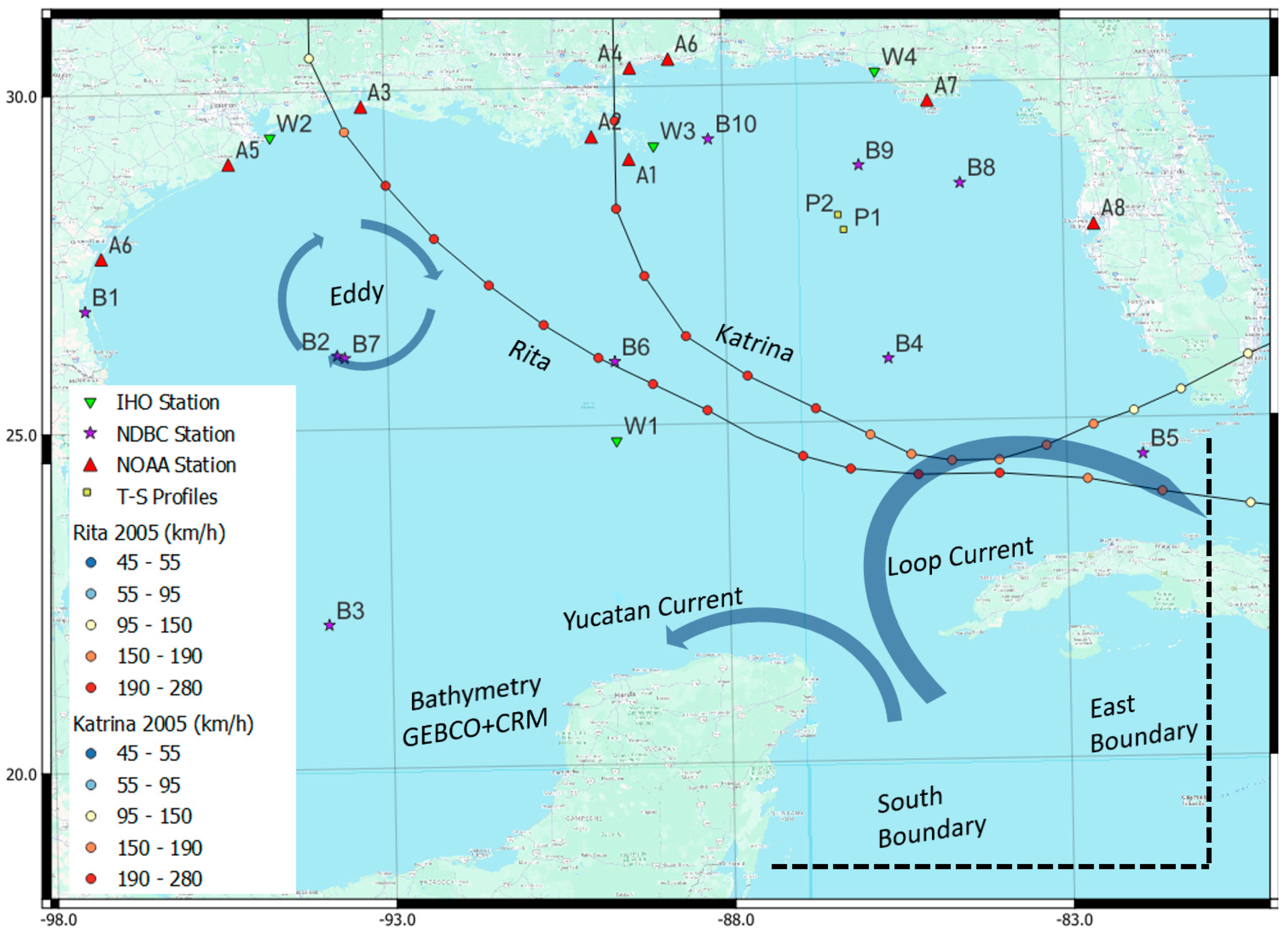
The Gulf of Mexico, situated between the Strait of Florida and the Yucatan Channel, stretches across the coordinates of 18–31° N and 99–81° W (Figure 1), representing a vast expanse of water. Its diverse terrain includes coastal regions, continental shelves and an abyssal plain, boasting an average depth of approximately 1615 m over its expansive 1.6 million km2 surface area [49]. Economically and ecologically, the Gulf holds significant importance both regionally and globally. Its rich energy resources support a thriving industry, with oil production reaching 1.65 million barrels per day in 2017 [50], sustaining over 55,000 jobs [51]. Additionally, the Gulf’s diverse marine ecosystems, including vibrant coral environments, harbor a plethora of marine species, underscoring its ecological significance [52].
The mixed layer depth (MLD) within the Gulf is of considerable importance for dynamic ocean management and fisheries applications. Understanding its fluctuations aids in predicting the distribution and abundance of marine life and informs management strategies amidst global climate change [53]. Due to the Gulf’s varied geological provinces at different depths, salinity and temperature exhibit notable seasonal variations. Salinity typically ranges between 30 and 36 ppt at a depth of 10 m due to coastal inflows, while deeper depths experience less variability at around 35.5–37 ppt. Likewise, sea surface temperatures vary seasonally, ranging from 28 to 29 °C in summer, from 16 to 18 °C in the northern Gulf and from 24 to 26 °C in the southern Gulf during winter [54]. Freshwater influx from the Mississippi river delta and other tributaries further influences salinity and temperature dynamics, particularly in the northern Gulf [55,56].
The Gulf’s physiographic diversity manifests in subtropical and tropical characteristics, driven by the Loop Current—a warm ocean current converging with the Yucatan and Florida currents [57,58,59]. This intricate circulation pattern, along with the Loop Current’s associated eddies, significantly impacts ocean circulation patterns [60,61,62] and biological communities [63,64] and even influences the development of hurricanes. Notably, hurricanes such as Katrina and Rita in 2005, intensifying rapidly over the warm waters of the Loop Current, highlight the Gulf’s vulnerability to extreme weather events [30,65,66]. Given the Gulf’s advantageous position for oceanographic and atmospheric observations, as well as its support for marine life and operational predictions across industrial, civilian and military sectors, significant weather events like hurricanes can profoundly impact these processes and environments. Investigating the spatial and temporal variability of the MLD under extreme weather events can enhance our understanding of the Gulf’s physical climate, offshore industrial operations and the maintenance of oceanic and atmospheric observations.
2.2. Hurricane Katrina (2005)
Hurricane Katrina, the impactful storm that struck the Gulf of Mexico in 2005, stands out as a suitable case study for this work due to its notable characteristics and significant socio-economic consequences along the Gulf Coast. Katrina exhibited remarkable strength, reaching Category 5 status with maximum sustained winds of 175 mph (280 km/h) and a center pressure of 902 mbar on 28 August. The trajectory of Hurricane Katrina presents a unique opportunity to examine the hydrographic responses of thermohaline processes to the intensification of wind forcing in the Gulf of Mexico. Initially, Katrina made landfall as a Category 1 hurricane on the southeastern coast of Florida. Subsequently, it rapidly intensified into a Category 3 hurricane within the Gulf, escalating to Category 5 status in less than 12 h. This swift intensification, coupled with fluctuations in strength as it progressed towards the northern Gulf coast, provides a dynamic scenario for investigating oceanographic responses. Furthermore, the profound impact of Hurricane Katrina on coastal communities and infrastructure underscores the importance of understanding the underlying oceanic dynamics during extreme weather events. Through our focus on Katrina, we aim to elucidate the complex interactions between atmospheric forcing and oceanic processes, shedding light on the mechanisms driving the intensification and propagation of tropical cyclones in the Gulf of Mexico. Our selection of Hurricane Katrina for this study is motivated by its exceptional characteristics, trajectory and socio-economic significance, which collectively provide a compelling basis for exploring the hydrographic responses of thermohaline processes in the Gulf region.
2.3. Model Configuration
We employ the Delft3D modeling system, integrating Delft3D-FLOW and Delft3D-WAVE modules [67], to investigate changes in thermohaline/thermocline characteristics induced by hurricanes in the Gulf of Mexico. Delft3D-FLOW, grounded in the three-dimensional Navier–Stokes equations for incompressible fluids, utilizes the Generalized Lagrangian Mean (GLM) formulation. In 3D mode, solutions are derived via the bottom-following σ- or fixed-level z-coordinate system, incorporating the shallow water approximation and Boussinesq approximation for buoyancy-driven flow. The model dynamically evolves hydrodynamics’ vertical structure, encompassing salinity, temperature, and resulting density gradients. Concurrently, the Delft3D-WAVE module integrates the Simulating WAves Nearshore (SWAN) model, a third-generation spectral wave model, to analyze wind–wave growth, wave–current interaction, dissipation and depth-induced surface wave breaking [68]. This module enables FLOW to access SWAN-modeled wave information, including wave orbital velocity, wave forcing and Stokes drift, while SWAN accesses surface currents and water levels from FLOW.
The model domain encompasses the entire Gulf of Mexico with open boundaries as shown in Figure 1. It is a spherical rectangular grid with a resolution of 0.04°×0.04° (~4 km) and vertical discretization of 40 vertical layers in the z-coordinate system. Layer thickness linearly increases from surface to bottom, with maximum layer thickness at 15.29% at the bottom and minimum at 0.03% at the surface. Combined bathymetry from the GEneral Bathymetric Chart of the Ocean [69] and Coastal Relief Model [70] is adopted in the model. In addition, we utilize the HYbrid Coordinate Ocean Model (HYCOM) + Navy Coupled Ocean Data Assimilation (NCODA) GoM 1/25° Reanalysis (GOMu0.04 expt_50.1 year-2005) data to provide the initial and boundary conditions. These data represent time- and space (via the layers)-varying boundary conditions of water level, current, salinity and temperature with high resolution (0.25°, ~3.5 km and 3 hourly) in the regional domain. Time series of Riemann invariants along the southern open boundary and current velocity along the eastern open boundary were used to simulate a weakly reflective boundary. The wave grid has a lower resolution of 0.1° × 0.1° (~10 km) and covers the hydrodynamic grid, with 24 frequency bins, ranging from 0.033 to 0.5 Hz, and 36 directional components. SWAN is run in non-stationary mode with a 10 min time-step and coupled with FLOW every 30 min. The coupled model simulation spans approximately 54 days from 1 July to 23 August with restart files containing the hydrodynamic conditions for the subsequent model runs.
Winds from the HRD Real-Time Hurricane Wind Analysis System (H*WIND, [71]) which provides high-accuracy and high-resolution wind field in a 4° × 4° grid around the center of the storm were combined with the winds from Coupled Ocean-Atmosphere Mesoscale Prediction System (COAMPS, [72,73]) for areas not covered by the H*WIND grid. This provided a more accurate wind field during extreme weather conditions, as compared with observed data from the National Data Buoy Center (NDBC) stations (as shown in Figure 2). The three wind drag coefficients are specified with the wind speed (0.001 at 0 m/s, 0.003 at 25 m/s, 0.00723 at 100 m/s) in Delft3D, and the k-ε 3D turbulence model is applied with constant horizontal eddy viscosity and diffusivity (10 m2/s). In addition, the Ocean Heat Flux model [74,75] typically applied for a large body of water [67] is used for the Gulf of Mexico. Several sources, including the COAMPS, National Centers for Environmental Prediction (NCEP) Climate Forecast System Reanalysis (CFSR) and Objectively Analyzed Air-Sea Fluxes (OAFlux), were incorporated to provide the meteorological data such as precipitation, evaporation air temperature, humidity and cloud coverage in the Gulf for the modeling system. These represent the three-hourly meteorological data over the entire Gulf of Mexico. In addition, the other specified physical parameters are given in Table 1.
The Multi-Directional Upwind Explicit (MDUE, [76]) scheme and Van-Leer 2 [77] method were used for momentum and transport solvers in the Z-coordinate system, respectively. In order to avoid computational noise, such as loss of imposing significant amplitude in a steeply peaked solution, the Forester filtering technique [78] was applied to smooth salinity and temperature variations in horizontal and vertical mixing. In addition, a slope limiter was used to prevent the large velocity gradients along the very steep bottom slopes.
2.4. Model Calibration
Multiple calibration steps were performed to achieve an optimal model configuration for thermohaline processes. These dynamical variables are influenced by various oceanographic conditions and expected to have a strong impact on thermohaline/thermocline predictions: Key parameters include eddy viscosity and diffusivity, Secchi depth and Dalton–Stanton number, which were selected based on values recommended in the model user’s manual or literature. Horizontal eddy viscosity and diffusivity are associated with three-dimensional turbulence eddies, horizontal motions, dispersion and forcing not resolved by the horizontal grid [67]. These values significantly contribute to salinity and temperature variations, affecting the characteristics of water mixing processes. Since they represent physics unresolved in the equations, they are utilized as calibration parameters. Recommended values vary widely, and we selected several sets of background horizontal eddy viscosity and diffusivity (1, 5, 10, 15 m2/s) to assess their impact. Secchi depth [79,80], as a measure of water transparency or turbidity in a body of water [81], is linked to the heat flux of net incident solar radiation. In the Ocean Heat Flux model, Secchi depth is used to compute the absorption of heat in the water column, influencing vertical mixing and thermohaline/thermocline structures [67]. The temporal and spatial incoming energy flux may induce vertical mixing and influence the thermohaline/thermocline structures. A number of studies [82,83,84,85,86,87] showed the significant effects of Secchi depth on temperature and salinity anomalies. The Secchi depths used here follow those used by FGDC [88]. The considered Secchi depths are 3.5, 5, 10 and 15 (m). Evaporation and heat exchange at the interface between ocean and air contribute significantly to the water temperature and salinity. Dalton and Stanton numbers are usually applied to compute the latent evaporative heat flux [67,89] and heat convection. In order to obtain a realistic hurricane simulation, the ratio of enthalpy to drag coefficient, (the range of 1.2~1.5, [90,91]), was applied to produce ensembles of Dalton and Stanton numbers in the calibration process. Here, is the exchange coefficient of heat which is a Dalton or Stanton number, and is surface drag coefficient. Table 2 provides a summary of the physical parameters in the calibration process.
2.5. Model Skill Metrics
These observations are depicted in Figure 1. Various error statistics, including root mean squared error (RMSE), Pearson’s correlation coefficient (CC) and refined index of agreement (RIA, [92]), were calculated for all available observed stations using data and model predictions.
Here, n = total number of data; = predicted model value; = observed field value; c is scale constant (c = 2, preferred). Several Taylor diagrams [93] provide a summary of the statistical results between each model result in calibration processes and observation. Three statistics are included: the RMS error of model results is represented by the grey dashed line; Pearson’s correlation coefficient (CC), which can quantify the similarity in pattern between modeled and observed points, is depicted in dashed–dotted contours; the refined index of agreement (RIA), proportional to the radial distance, is shown in dashed contours. The predicted water level and vertical profiles of salinity and temperature were compared to four tidal stations, two vertical profiles and HYCOM results. Figure 3 and Figure 4 show the results of total error statistics for water level change and vertical profiles, respectively. Although no obvious trends emerge due to the different parameters, minimal impact is observed across the range of values chosen, even for the background eddy viscosity and diffusivity. However, certain stations tend to exhibit better performance with specific sets of values. A combination of specified forcing using the optimal parameter set, with the values of 10/10 (m2/s) for eddy viscosity and diffusivity, 10 m for Secchi depth and 0.0041/0.0041 for Dalton and Stanton number (Table 2), was utilized for the results presented in the remainder of this study.
3. Results
3.1. Model Validations—Water Levels, Winds and Waves
A total of six NOAA tidal stations (station locations in Table 3) were used to compare the water elevation with the model results (as shown in Figure 5) along the Louisiana and Mississippi coasts during Hurricane Katrina. Water levels at stations Norco, B Labranche (#A3) and Cypremort Point (#A4) were somewhat over- and under-estimated, respectively, during the hurricane event, but the other four stations in open water show great agreement, which boosts confidence in our model results.
The predicted significant wave height and wave peak period were compared with observed data from NDBC stations in Figure 6. The model exhibits great performance over the buoy stations in the eastern Gulf (right side of storm track). Minor differences in significant wave height and peak period are attributable to wind uncertainty, currents and bathymetry profile. However, the significant wave heights observed at stations 42,001 (#B6) and 42,002 (#B7) are notably smaller than the model results, likely due to the hurricane’s counter-clockwise rotation leading to less energetic waves to the left side of the eye because these waves encounter opposing winds and absorb less energy from them [94], which is likely to have a significant impact on the development of wave height. However, this effect is not accounted for in SWAN and consequently results in larger than observed wave height predictions. Overall, the coupled model (Delft3D FLOW+WAVE) agrees well with the measured wave and wind parameters at NDBC stations as shown in Figure 6. Table 3 gives the summary of statistical results for water levels and vertical profiles.
3.2. Model Validations—Vertical Profiles of Salinity and Temperature
Only two observed vertical profiles (in Figure 1) were available during July and August in 2005. Figure 7 shows the comparisons of vertical profiles for the salinity and temperature on 10 and 19 July. The model demonstrates a good agreement with the observed value, except for the surface anomaly in salinity for 10 July. In addition, the model results align with the HYCOM reanalysis data which provided the salinity and temperature conditions initially in the entire domain and along the boundary during the simulation. The RMSE was 0.46 ppt/0.84 °C on 10 July and 0.26 ppt/0.7 °C on 19 July. One drawback in the model validation is insufficient historical profile data during the period of time in this study, but the agreement of the model results with available measurements of water levels/winds/waves lends confidence in the model. To ensure the adequacy of model configurations and the model’s ability to accurately simulate hydrodynamic and thermohaline processes, we compared profiles across various locations within the model domain to HYCOM reanalysis data. This comparison is depicted in Figure 7, demonstrating relatively good agreement between our model and HYCOM at multiple locations. In addition, the comparison of sea surface height from the model and altimetry (shown in Figure 8) can support whether the model accurately represents pertinent ocean circulation in terms of spatial and temporal distribution and current intensity. The satellite-based radar altimetry measurements of the sea surface height anomaly (SSHA) from satellites such as TOPography EXperiment (TOPEX)/Poseidon, European Remote Sensing Satellite (ERS-1, ERS-2), Geosat Follow-On, Envisat and Jason-1 are merged into daily gridded data maps and utilized for comparison with the surface water elevation from the model. By aligning our model results with data from these satellite altimeters, which provide measurements based on the geoid representing mean sea level, we can directly evaluate the performance of the model in reproducing sea surface height variations. This comparison helps in determining whether the model (its performance) has the relevant ocean circulations and processes in the right place and with the right current strength. Figure 8 shows the comparison between daily mean water levels from the model and daily altimetry data. The correlation between the daily mean water level and sea surface height anomaly was estimated to be between 0.78 and 0.91 over the Gulf of Mexico for the given period. Additionally, salinity/temperature profiles and water level observations serve as validation metrics for the model.
3.3. Vertical Variability of Salinity and Temperature
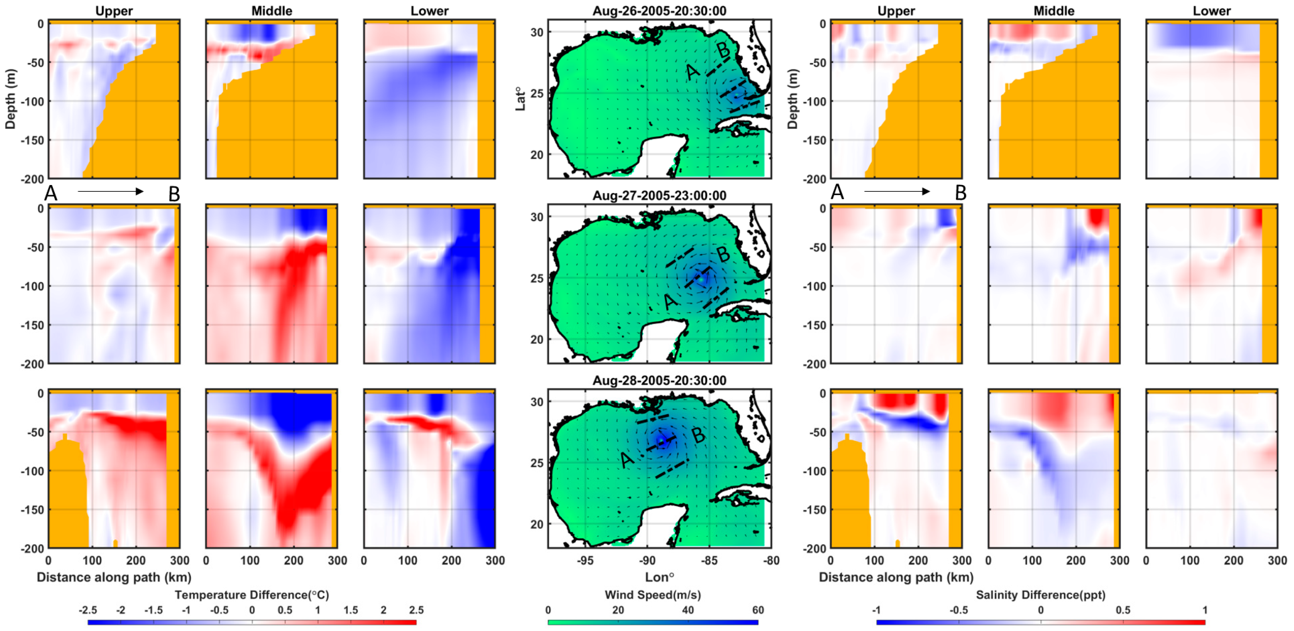
Figure 9 and Figure 10 show the temperature and salinity differences following Hurricane Katrina’s passage, delineating the left and right sides of the storm, as well as ahead of the eye and in the wake at various times within the upper 200 m in depth. As shown in Figure 9, the stronger wind force on the right side of the storm’s eye induces horizontal and vertical temperature changes of ±4 °C and salinity changes of ±1.5 ppt after Katrina’s passage at 20:30:00 on 28 August. Conversely, Figure 10 depicts spatial and temporal variations along the eye at the same time, showcasing an increase and decrease of ~±2.5 °C in temperature and ~± 1.0 ppt in salinity due to the strong hurricane winds and influx of warm water possibly associated with the Loop Current. Temperature and salinity differences were calculated relative to a three-day mean sea state (21–23 August) preceding the storm. As shown in both figures, the water mass exchanges driven by the strong winds drive the various processes, such as disturbance, mixing and transport, leading to abrupt changes in temperature and salinity. The turbulence caused by the strong wind-driven current in the upper ocean can uplift colder water from the thermocline to the mixed layer, resulting in thickening and cooling [95]. Although the likelihood of upwelling process influence is not significantly higher [96], the combination of turbulence-driven vertical mixing and enhanced upwelling caused by geostrophic flow, such as the Loop Current and frontal cyclones [30,97], contributes to cooling beneath the storm. This effect is particularly pronounced on the right side of the eye, as depicted in Figure 10. Salinity anomalies are less distinct compared to temperature. Typically, salinity increases gradually with depth. However, during Hurricane Katrina, intense vertical mixing led to salinity increases in the mixed layer due to the intense entrainment of high salinity from the subsurface layer [24,98,99,100]. Additionally, the energy absorbed from the environment during the evaporation process can likely lead to cooling of the upper ocean layer and salinization of the ocean mixed layer [101], as observed in the results for 28 August at 20:30:00 in Figure 10.
3.4. Mixed Layer Depth during Katrina
A simple threshold approach [16,102,103,104,105] is utilized to identify the MLD from model results based on a temperature variation of 0.2 °C from the surface/reference depth. The strong current generated by hurricane winds, along with mixing induced by waves and turbulence in the upper ocean layer, significantly influence temperature variations during extreme weather events [45,48,106,107,108]. Dynamic cooling and dissipative heating processes at the surface layer also drive these variations [41,42], subsequently affecting the transport of heat flux and the thermocline structure [43]. Figure 11 illustrates the distribution of daily mean mixed layer depth relative to the development of hurricane winds. Figure 11(a1) depicts the initial phases of the wind field and the mean MLD over three days preceding the storm (21–23 August). Utilizing a temperature variation of 0.2 °C, we observe a pre-storm MLD ranging from 20 to 40 m (Figure 11), consistent with seasonal values. Notably, the MLD substantially deepens to around 120 m on 29–30 August in the middle of the northeastern Gulf. As discussed below, the MLD gradually returns to pre-hurricane conditions following the passage of Hurricane Katrina.
4. Further Discussion
4.1. MLD Recovery
The recovery of the MLD from storm disturbances appears to vary depending on the background climate [109]. Understanding the degree (e.g., duration) it takes for the MLD to revert to pre-storm levels aids in comprehending the upper ocean’s response to storms. The relative change in the MLD, expressed as a percentage (%), is calculated using the equation
where represents the mean MLD computed over the two days preceding the storm impact and is the MLD at time i after the storm’s passage. Figure 12 presents the Gulf’s MLD change resulting from several hurricanes, encompassing the period from July to August (before Katrina) and extending to September 2005, based on MLD variations attributable to each storm’s impact. Mean MLD distributions during 1–2 July (a) and 21–22 August (b) serve as benchmarks for determining MLD changes induced by hurricane impacts. Following Hurricane Cindy, a Category 1 storm with maximum winds of 33.4 m/s that traversed from south to north across the middle of the Gulf, the Gulf failed to fully return to its normal sea state due to the subsequent Hurricane Dennis. Post-Cindy, the MLD recovered to approximately 81%, but it subsequently dropped to 72% following Dennis’s impact. Despite Dennis being upgraded to a Category 3–4 hurricane, it resulted in only a 9% additional decrease from Cindy’s impact, with the MLD recovering to 79% by 16–17 July. Due to Dennis’s more eastern storm track, the shallow depth and continental shelf regions along the western side of the Florida Panhandle were likely unaffected in terms of MLD evolution. Hurricane Emily, reaching Category 5 intensity in the Caribbean Sea, drove warm water through the Yucatan Channel, inducing anomalously high temperatures and salinity [110], before moving west to northwest. Emily’s impact led to a significant MLD decrease to 55–57%, gradually rebounding to over 75% post-storm. Even during the interlude between Hurricanes Emily and Katrina, the Gulf’s MLD had not fully recovered, remaining below 80%. The cumulative impact of multiple storms within a short period may compromise the Gulf’s oceanic hydrodynamic resilience, altering the region’s climate background.
In Figure 12b, two different mean-MLD bases are utilized, computed during 1–2 July and 21–22 August. Compared to the preceding hurricanes, Katrina inflicted the most substantial MLD impact, with the MLD level plummeting to 37–39% using the July basis. Even three weeks later (before Hurricane Rita), the MLD level remained below 70%. Katrina’s influence was anticipated to cause significant changes in thermohaline processes, circulation and mixing during and after impact. When compared to the August basis, Katrina still induced a substantial MLD change of 60%, with an eventual recovery to approximately 84%. The Gulf had not fully rebounded from Katrina’s impact and was subsequently affected by Hurricane Rita on 20 September (not examined here). A longer duration may be necessary for the Gulf to recover to over 90% of its former sea state, but multiple hurricane strikes during the Atlantic hurricane season impede full recovery.
4.2. Wave Effect on MLD
A strong hurricane event is expected to have a major impact on mixing and transport via surface waves. However, the influence of waves on the thermohaline structure and the subsequent impacts of white-capping on said structure remain areas of ongoing investigation [111]. To address this gap, we utilized both model results from FLOW and the coupled FLOW+WAVE to scrutinize the wind-driven wave effect on parameters such as the mixed layer depth (MLD), temperature and salinity.
In Figure 13, we present comparisons of daily mean MLD distributions during Hurricane Katrina, contrasting results from the FLOW and FLOW+WAVE coupled models. Additionally, we depict wave length and MLD along a cross-section down the long axis of the Gulf at each time step. During the early stages of the storm on 26 August, the MLDs showed minimal response to the waves. However, the intense hurricane wind-driven waves on 28–29 August led to more significant variations in MLD in the northeastern Gulf of Mexico compared to predictions without wave effects. Notably, on 30 August, even as Hurricane Katrina weakened while moving inland over southern and central Mississippi, both models estimated wider and deeper MLDs, hinting at the persistent influence of the storm’s dynamics.
Various hydrodynamic and wave characteristics, such as time lag for MLD response to strong winds and wave dynamics, as well as geological features and circulations, may account for this phenomenon. Typically, wave effects penetrate to a depth of half their wavelength [112,113], with predicted wavelengths in ranges conducive to affecting the MLD, as depicted in Figure 13. We observe that strong wind-driven waves result in deeper MLDs, approximately 3.5–5.4% deeper than those predicted by the FLOW model alone (Figure 13). Although the additional mixing induced by wave effects may appear minor, it provides invaluable insights into the contribution of wave-induced processes to overall mixing. Even at a relatively small scale of 3.5–5.4%, this understanding is important for systems reliant on acoustic (sonar) technology, which is highly sensitive to temperature and density variations. Recognizing and comprehending the impact of waves on oceanic processes, such as the MLD, allows stakeholders to improve their interpretation and adapt their strategies for navigation, ocean monitoring and environmental assessment in storm-prone regions like the Gulf of Mexico.
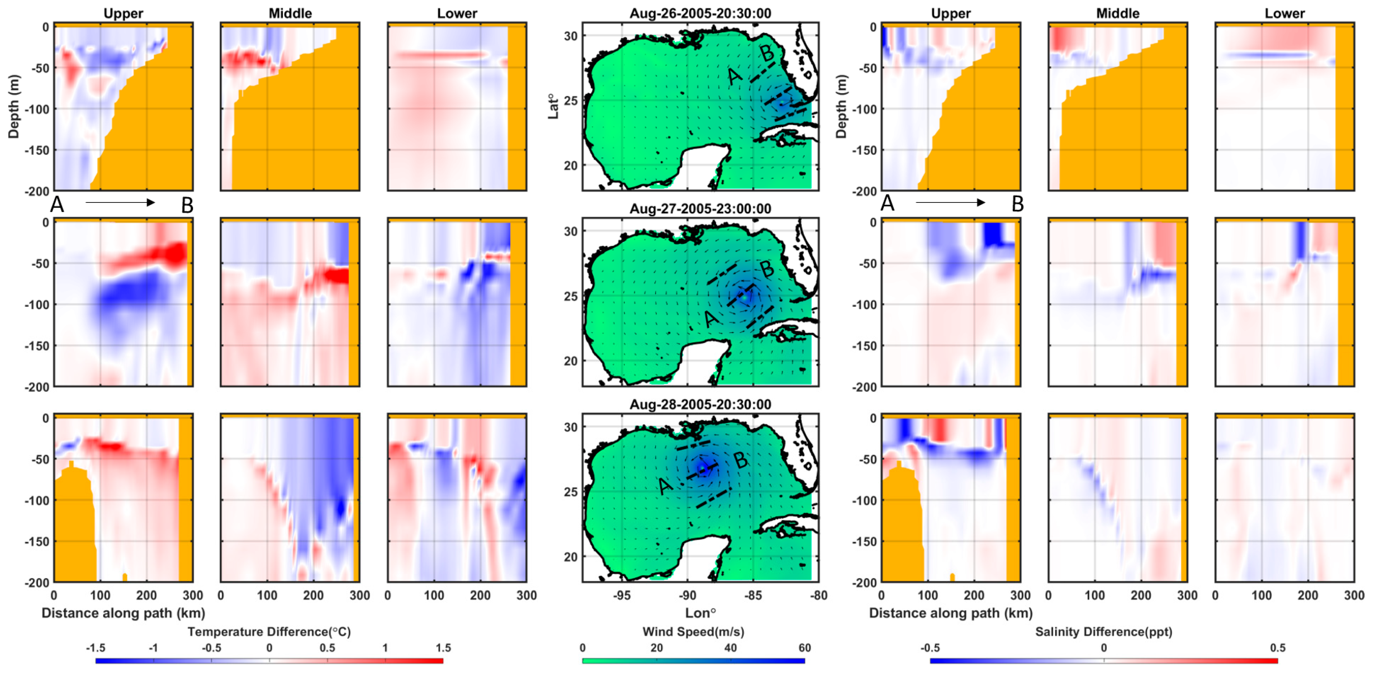
Figure 14 and Figure 15 illustrate vertical variations in temperature and salinity caused by wind-driven wave effects during Hurricane Katrina. These figures compare differences in temperature and salinity between the coupled FLOW+WAVE model and the FLOW model cross-sections along the specified lines. The coupled model results demonstrate greater depth variations in temperature and salinity due to surface waves. While no significant changes occur in the salinity field, the coupled model reveals spatial and temporal variations, with temperature fluctuations of up to ±2.0 °C and salinity fluctuations of up to ±1.0 ppt compared to FLOW model results. Additionally, strong winds on the right side of the storm track exhibit a more pronounced effect on temperature and salinity fields than those on the left side of the eye. The wave effects on the thermohaline process cross-sections, as depicted in Figure 14 and Figure 15, can be inferred from the model predictions between the MLDs and associated wavelengths in Figure 13. These effects are likely attributable to dynamic cooling, dissipative heating and wave processes acting as turbulent sources on the ocean surface [42,114,115].
5. Conclusions
This study provides a comprehensive analysis of the hydrodynamic and wave effects of Hurricane Katrina on the Gulf of Mexico’s upper ocean dynamics. Utilizing a sophisticated modeling system integrating Delft3D FLOW and WAVE models, we evaluated various parameters including water elevation, vertical profiles of salinity and temperature, significant wave height, peak period, wind speed and direction. Our findings indicate strong agreement between model predictions and observational data from NOAA, NDBC, TOPEX and ERS-2 satellites, as well as the HYCOM model used for initial and boundary conditions.
During Hurricane Katrina, the model accurately captured spatial and temporal variations in temperature and salinity, with notable increases and decreases observed. Under the influence of extreme weather conditions, such as Hurricane Katrina, significant cooling, wind-driven mixing and surface heat loss induce notable spatial and temporal variations in temperature (~±4 °C) and salinity (~±1.5 ppt). The MLD is strongly developed with ~120 m (or more) on 29–30 August in the middle of the northeastern Gulf, compared to pre-storm conditions (~20–40 m). Recovery analysis indicates that it takes about 18 days for the MLD to rebound to approximately 84% of its pre-storm level following Hurricane Katrina. Additionally, the incorporation of surface wave effects in the coupled model results in a slightly deeper MLD (~5%) compared to the stand-alone hydrodynamic model. Our findings underscore the importance of accurate modeling in predicting and understanding the impacts of extreme weather events on ocean dynamics. These provide valuable insights for scientific understanding, environmental management and operation applications, particularly in predicting and mitigating the impacts of extreme weather events on ocean dynamics.
Future applications should focus on incorporating denser observational data to further refine and validate the model, facilitating deeper insights into the complex responses of thermohaline structure and circulation to hurricane-induced disturbances. By leveraging advanced modeling techniques and observational data, we can deepen our understanding of marine systems and inform strategies for mitigating the impacts of climate-related disasters.
Author Contributions
W.L. designed the concept and methodology of the integrated modeling system, constructed the Delft3D model and performed Delft3D model validations. W.L. analyzed the model results and provided the initial draft of the manuscript. J.V. contributed in supporting the modeling technique and discussing, editing and writing processes. All authors actively contributed to analyzing model outcomes and revisions in the writing process. All authors have read and agreed to the published version of the manuscript.
Funding
The research presented in this paper was funded by the Office of Naval Research (ONR, Grant No. N0001421WX00991).
Institutional Review Board Statement
Not applicable.
Informed Consent Statement
Not applicable.
Data Availability Statement
All datasets used in this study are publicly available: (a) GEBCO and CRM bathymetry data are available at https://www.bodc.ac.uk/data/hosted_data_systems/gebco_gridded_bathymetry_data/ (accessed on 15 April 2022) and https://www.ngdc.noaa.gov/mgg/coastal/crm.html, (accessed on 15 April 2022) respectively; (b) NCEP-CFSR (https://rda.ucar.edu/datasets/ds093.1/) (accessed on 15 April 2022) and OAFlux (https://rda.ucar.edu/datasets/ds260.1/) (accessed on 15 April 2022) provide the meteorological data in Gulf of Mexico for model input of heat flux; (c) the HYCOM+NCODA reanalysis data provided by U.S. Navy are available at http://tds.hycom.org/thredds/catalogs/GOMu0.04/expt_50.1.html?dataset=GOMu0.04-expt_50.1-2005 (accessed on 20 April 2022); (d) U.S. Naval research laboratory provided the COAMPS data, and HRD real-time hurricane analysis data HWIND are available at https://www.rms.com/event-response/hwind/legacy-archive (accessed on 22 April 2022); (e) profile data of temperature and salinity are obtained from the Naval Oceanographic Office, where profiles from Argo drifters, ship-based XBTs and CTDs, gliders, and fixed and drifting buoys obtained from the GTS system are processed for operational use; (f) the historical meteorological data and tides/water level in the Gulf of Mexico were obtained from NOAA’s NDBC (https://www.ndbc.noaa.gov) (accessed on 23 April 2022) and NOAA’s Tides and Currents (https://tidesandcurrents.noaa.gov) (accessed on 23 April 2022), respectively; (g) sea surface height anomaly (SSH-A) from the TOPography EXperiment (TOPEX) and European Remote Sensing Satellite (ERS-2) is available at https://geo.gcoos.org/ssh/data1/ (accessed on 23 May 2022).
Acknowledgments
The authors thank all collaborators for sharing data sources and interactive discussion. The authors would like to thank anonymous reviewers for their valuable feedback during the submission and editing process of this manuscript.
Conflicts of Interest
The authors declare no conflicts of interest/competing interests.
References
- Chen, D.; Busalacchi, A.J.; Rothstein, L.M. The roles of vertical mixing, solar radiation, and wind stress in a model simulation of the sea surface temperature seasonal cycle in the tropical Pacific Ocean. J. Geophys. Res. 1994, 99, 20345–20359. [Google Scholar] [CrossRef]
- Sutton, P.J.; Worcester, P.F.; Masters, G.; Cornuelle, B.D.; Lynch, J.F. Ocean mixed layers and acoustic pulse propagation in the Greenland Sea. J. Acoust. Soc. Am. 1993, 94, 1517–1526. [Google Scholar] [CrossRef]
- Arrigo, K.R.; Robinson, D.H.; Worthen, D.L.; Dunbar, R.B.; Ditullio, G.R.; Vanwoert, M.; Lizotte, M.P. Phytoplankton community structure and the drawdown of nutrients and CO2 in the southern ocean. Science 1999, 283, 365–367. [Google Scholar] [CrossRef] [PubMed]
- Fasham, M.J.R. Variations in the seasonal cycle of biological production in subarctic oceans: A model sensitivity analysis. Deep Sea Res. Part I Oceanogr. Res. Pap. 1995, 42, 1111–1149. [Google Scholar] [CrossRef]
- Helber, R.W.; Kara, A.; Barron, C.; Boyer, T. Mixed layer depth in the Aegean, Marmara, Black and Azov Seas: Part II: Relation to the sonic layer depth. J. Mar. Syst. 2009, 78, S181–S190. [Google Scholar] [CrossRef]
- Obata, A.; Ishizaka, J.; Endoh, M. Global verification of critical depth theory for phytoplankton bloom with climatological in situ temperature and satellite ocean color data. J. Geophys. Res. Oceans 1996, 101, 20657–20667. [Google Scholar] [CrossRef]
- Polovina, J.J.; Mitchum, G.T.; Evans, G.T. Decadal and basin-scale variation in mixed layer depth and the impact on biological production in the Central and North Pacific, 1960–1988. Deep Sea Res. Part I Oceanogr. Res. Pap. 1995, 42, 1701–1716. [Google Scholar] [CrossRef]
- Agrawal, Y.C.; Terray, E.A.; Donelan, M.A.; Hwang, P.A.; Williams, A.J.; Drennan, W.M.; Kahma, K.K.; Krtaigorodskii, S.A. Enhanced dissipation of kinetic energy beneath surface waves. Nature 1992, 359, 219–220. [Google Scholar] [CrossRef]
- Craik, A.D.; Leibovich, S. A rational model for Langmuir circulations. J. Fluid Mech. 1976, 73, 401–426. [Google Scholar] [CrossRef]
- Large, W.G.; McWilliams, J.C.; Doney, S.C. Oceanic vertical mixing: A review and a model with a nonlocal boundary layer parameterization. Rev. Geophys. 1994, 32, 363–403. [Google Scholar] [CrossRef]
- Mellor, G.L.; Durbin, P.A. The structure and dynamics of the ocean surface mixed layer. J. Phys. Oceanogr. 1975, 5, 718–728. [Google Scholar] [CrossRef]
- Pickard, G.; Emery, W. Descriptive Physical Oceanography: An Introduction By George L. Pickard Oxford: Pergamon Press1964. Pp. viii + 199. Price 25s. J. Mar. Biol. Assoc. UK 1964, 44, 758. [Google Scholar]
- Roden, G.I. The Depth Variability of Meridional Gradients of Temperature, Salinity and Sound Velocity in the Western North Pacific. J. Phys. Oceanogr. 1979, 9, 756–767. [Google Scholar] [CrossRef]
- Skyllingstad, E.D.; Paluszkiewicz, T.; Denbo, D.W.; Smyth, W.D. Nonlinear vertical mixing processes in the ocean: Modeling and parameterization. Phys. D Nonlinear Phenom. 1996, 98, 574–593. [Google Scholar] [CrossRef]
- Welander, P. Mixed Layers and Fronts in Simple Ocean Circulation Models. J. Phys. Oceanogr. 1981, 11, 148–152. [Google Scholar] [CrossRef]
- de Boyer Montégut, C.; Madec, G.; Fischer, A.S.; Lazar, A.; Iudicone, D. Mixed layer depth over the global ocean: An examination of profile data and a profile-based climatology. J. Geophys. Res. Ocean. 2004, 109. [Google Scholar] [CrossRef]
- Spall, M.A.; Weller, R.A.; Furey, P.W. Modeling the three-dimensional upper ocean heat budget and subduction rate during the Subduction Experiment. J. Geophys. Res. Ocean. 2000, 105, 26151–26166. [Google Scholar] [CrossRef]
- Thomson, R.E.; Fine, I.V. Estimating Mixed Layer Depth from Oceanic Profile Data. J. Atmos. Ocean. Technol. 2003, 20, 319–329. [Google Scholar] [CrossRef]
- Bhaskar, T.U.; Swain, D. Sonic Layer Depth estimated from XBT temperatures and climatological salinities. Nat. Preced. 2011. [Google Scholar] [CrossRef]
- Huang, R.X. Ocean Circulation: Wind-Driven and Thermohaline Processes; Cambridge University Press: Cambridge, UK, 2010. [Google Scholar]
- Murty, T.S.; El-Sabh, M.I. Storm tracks, storm surges and sea state in the Arabian Gulf, Strait of Hormuz and the Gulf of Oman. UNESCO Rep. Mar. Sci 1984, 28, 12–24. [Google Scholar]
- Schott, F.; Visbeck, M.; Send, U.; Fischer, J.; Stramma, L.; Desaubies, Y. Observations of deep convection in the Gulf of Lions, northern Mediterranean, during the winter of 1991/92. J. Phys. Oceanogr. 1996, 26, 505–524. [Google Scholar] [CrossRef]
- Lee, C.M.; Askari, F.; Book, J.; Carniel, S.; Cushman-Roisin, B.; Dorman, C.; Doyle, J.; Flament, P.; Harris, C.K.; Jones, B.H. Northern Adriatic response to a wintertime bora wind event. Eos Trans. Am. Geophys. Union 2005, 86, 157–165. [Google Scholar] [CrossRef]
- Jacob, S.D.; Shay, L.K.; Mariano, A.J.; Black, P.G. The 3D Oceanic Mixed Layer Response to Hurricane Gilbert. J. Phys. Oceanogr. 2000, 30, 1407–1429. [Google Scholar] [CrossRef]
- Shay, L.; Black, P.; Mariano, A.; Hawkins, J.; Elsberry, R. Upper ocean response to Hurricane Gilbert. J. Geophys. Res. Ocean. 1992, 97, 20227–20248. [Google Scholar] [CrossRef]
- Shay, L.K.; Goni, G.J.; Black, P.G. Effects of a Warm Oceanic Feature on Hurricane Opal. Mon. Weather Rev. 2000, 128, 1366–1383. [Google Scholar] [CrossRef]
- Uhlhorn, E.W.; Shay, L.K. Loop Current Mixed Layer Energy Response to Hurricane Lili (2002). Part I: Observations. J. Phys. Oceanogr. 2012, 42, 400–419. [Google Scholar] [CrossRef]
- Walker, N.D.; Leben, R.R.; Balasubramanian, S. Hurricane-forced upwelling and chlorophyll a enhancement within cold-core cyclones in the Gulf of Mexico. Geophys. Res. Lett. 2005, 32. [Google Scholar] [CrossRef]
- Jaimes, B.; Shay, L.K. Near-Inertial Wave Wake of Hurricanes Katrina and Rita over Mesoscale Oceanic Eddies. J. Phys. Oceanogr. 2010, 40, 1320–1337. [Google Scholar] [CrossRef]
- Jaimes, B.; Shay, L.K. Mixed layer cooling in mesoscale oceanic eddies during Hurricanes Katrina and Rita. Mon. Weather Rev. 2009, 137, 4188–4207. [Google Scholar] [CrossRef]
- Shay, L.K. Upper Ocean Structure: Responses to Strong Atmospheric Forcing Events. In Encyclopedia of Ocean Sciences; Elsevier Ltd.: Amsterdam, The Netherlands, 2009; pp. 192–210. Available online: http://www.scopus.com/inward/record.url?scp=84884459695&partnerID=8YFLogxK (accessed on 12 November 2021).
- Fedorov, K.N.; Varfolomeev, A.A.; Ginzburg, A.I. Thermal reaction of the ocean on the passage of hurricane Ella. Okeanologiya 1979, 19, 992–1001. [Google Scholar]
- Leipper, D.F. Observed ocean conditions and Hurricane Hilda, 1964. J. Atmos. Sci. 1967, 24, 182–186. [Google Scholar] [CrossRef]
- Black, P.G. Ocean temperature changes induced by tropical cyclones. Ph.D. Thesis, The Pennsylvania State University, State College, PA, USA, 1983. [Google Scholar]
- Brooks, D.A. The wake of Hurricane Allen in the western Gulf of Mexico. J. Phys. Oceanogr. 1983, 13, 117–129. [Google Scholar] [CrossRef]
- Shay, L.K.; Elsberry, R.L. Near-inertial ocean current response to Hurricane Frederic. J. Phys. Oceanogr. 1987, 17, 1249–1269. [Google Scholar] [CrossRef]
- Bender, M.A.; Ginis, I.; Kurihara, Y. Numerical simulations of tropical cyclone-ocean interaction with a high-resolution coupled model. J. Geophys. Res. Atmos. 1993, 98, 23245–23263. [Google Scholar] [CrossRef]
- Gierach, M.M.; Subrahmanyam, B.; Thoppil, P.G. Physical and biological responses to Hurricane Katrina (2005) in a 1/25 nested Gulf of Mexico HYCOM. J. Mar. Syst. 2009, 78, 168–179. [Google Scholar] [CrossRef]
- Davis, C.; Wang, W.; Chen, S.S.; Chen, Y.; Corbosiero, K.; DeMaria, M.; Dudhia, J.; Holland, G.; Klemp, J.; Michalakes, J.; et al. Prediction of Landfalling Hurricanes with the Advanced Hurricane WRF Model. Mon. Weather Rev. 2008, 136, 1990–2005. [Google Scholar] [CrossRef]
- Halliwell Jr, G.R.; Shay, L.K.; Jacob, S.D.; Smedstad, O.M.; Uhlhorn, E.W. Improving ocean model initialization for coupled tropical cyclone forecast models using GODAE nowcasts. Mon. Weather Rev. 2008, 136, 2576–2591. [Google Scholar] [CrossRef]
- Korty, R.L.; Emanuel, K.A.; Scott, J.R. Tropical cyclone–induced upper-ocean mixing and climate: Application to equable climates. J. Clim. 2008, 21, 638–654. [Google Scholar] [CrossRef]
- Liu, H.-L. Temperature changes due to gravity wave saturation. J. Geophys. Res. 2000, 105, 12329–12336. [Google Scholar] [CrossRef]
- Bueti, M.R.; Ginis, I.; Rothstein, L.M.; Griffies, S.M. Tropical cyclone–induced thermocline warming and its regional and global impacts. J. Clim. 2014, 27, 6978–6999. [Google Scholar] [CrossRef]
- Jacob, S.D.; Shay, L.K. The Role of Oceanic Mesoscale Features on the Tropical Cyclone–Induced Mixed Layer Response: A Case Study. J. Phys. Oceanogr. 2003, 33, 649–676. [Google Scholar] [CrossRef]
- Mao, Q.; Chang, S.W.; Pfeffer, R.L. Influence of large-scale initial oceanic mixed layer depth on tropical cyclones. Mon. Weather Rev. 2000, 128, 4058–4070. [Google Scholar] [CrossRef]
- McPhaden, M.J.; Foltz, G.R.; Lee, T.; Murty, V.S.N.; Ravichandran, M.; Vecchi, G.A.; Vialard, J.; Wiggert, J.D.; Yu, L. Ocean-Atmosphere Interactions During Cyclone Nargis. Eos Trans. Am. Geophys. Union 2009, 90, 53–54. [Google Scholar] [CrossRef]
- Sutyrin, G.G.; Khain, A.P. Effect of the ocean–atmosphere interaction on the intensity of a moving tropical cyclone. Atmos. Ocean. Phys. 1984, 20, 787–794. [Google Scholar]
- Toffoli, A.; McConochie, J.; Ghantous, M.; Loffredo, L.; Babanin, A.V. The effect of wave-induced turbulence on the ocean mixed layer during tropical cyclones: Field observations on the Australian North-West Shelf. J. Geophys. Res. Ocean. 2012, 117, C00J24. [Google Scholar] [CrossRef]
- Nipper, M.; Sánchez Chávez, J.A.; Tunnell, J.W., Jr. (Eds.) Gulf Base: Resource Database for Gulf of Mexico Research; World Wide Web Electronic Publication, 2009; Available online: http://www.gulfbase.org (accessed on 10 March 2022).
- U.S. Energy Information Administration. U.S. Gulf of Mexico Crude Oil Production to Continue at Record Highs through 2019. 2018. Available online: https://www.eia.gov/todayinenergy/detail.php?id=35732 (accessed on 10 March 2022).
- Hill, K.; Hill, G.N. Encyclopedia of Federal Agencies and Commissions; Infobase Publishing: New York, NY, USA, 2014. [Google Scholar]
- Kennedy, J. Facts about Marine Life in the Gulf of Mexico. Thought Co, 26 February 2019. Available online: https://www.thoughtco.com/gulf-of-mexico-facts-2291771 (accessed on 13 September 2019).
- Hobday, A.J.; Hartog, J.R. Derived Ocean Features for Dynamic Ocean Management. Oceanography 2014, 27, 134–145. [Google Scholar] [CrossRef]
- Baranova, O.; Biddle, M.; Boyer, T. Seawater Temperature–Climatological Mean In Gulf of Mexico Data Atlas. Stennis Space Center (MS): National Centers for Environmental Information. 2014. Available online: https://gulfatlas.noaa.gov/ (accessed on 20 June 2022).
- Lane, R.R.; Day, J.W.; Marx, B.D.; Reyes, E.; Hyfield, E.; Day, J.N. The effects of riverine discharge on temperature, salinity, suspended sediment and chlorophyll a in a Mississippi delta estuary measured using a flow-through system. Estuar. Coast. Shelf Sci. 2007, 74, 145–154. [Google Scholar] [CrossRef]
- McDonald, T.; Telander, A.; Marcy, P.; Oehrig, J.; Geggel, A.; Roman, H.; Powers, S. Temperature and Salinity Estimation in Estuaries of the Northern Gulf of Mexico. NOAA Tech Rep. 2015. Available online: https://www.fws.gov/doiddata/dwh-ar-documents/863/DWH-AR0270936.pdf (accessed on 1 March 2022).
- Gyory, J.; Mariano, A.J.; Ryan, E.H. The Loop Current. Ocean Surface Currents. 2019. Available online: https://oceancurrents.rsmas.miami.edu/atlantic/loop-current.html (accessed on 1 March 2022).
- Hofmann, E.E.; Worley, S.J. An investigation of the circulation of the Gulf of Mexico. J. Geophys. Res. Ocean. 1986, 91, 14221–14236. [Google Scholar] [CrossRef]
- Sturges, W.; Leben, R. Frequency of Ring Separations from the Loop Current in the Gulf of Mexico: A Revised Estimate. J. Phys. Oceanogr. 2000, 30, 1814–1819. [Google Scholar] [CrossRef]
- Liu, Y.; Weisberg, R.H.; Vignudelli, S.; Mitchum, G.T. Patterns of the loop current system and regions of sea surface height variability in the eastern Gulf of Mexico revealed by the self-organizing maps. J. Geophys. Res. Ocean. 2016, 121, 2347–2366. [Google Scholar] [CrossRef]
- Pérez-Brunius, P.; Furey, H.; Bower, A.; Hamilton, P.; Candela, J.; García-Carrillo, P.; Leben, R. Dominant Circulation Patterns of the Deep Gulf of Mexico. J. Phys. Oceanogr. 2018, 48, 511–529. [Google Scholar] [CrossRef]
- Weisberg, R.H.; Liu, Y. On the Loop Current Penetration into the Gulf of Mexico. J. Geophys. Res. Ocean. 2017, 122, 9679–9694. [Google Scholar] [CrossRef]
- Davis, R.W.; Ortega-Ortiz, J.G.; Ribic, C.A.; Evans, W.E.; Biggs, D.C.; Ressler, P.H.; Cady, R.B.; Leben, R.R.; Mullin, K.D.; Würsig, B. Cetacean habitat in the northern oceanic Gulf of Mexico. Deep Sea Res. Part I Oceanogr. Res. Pap. 2002, 49, 121–142. [Google Scholar] [CrossRef]
- Love, M.; Baldera, A.; Yeung, C.; Robbins, C. The Gulf of Mexico Ecosystem: A Coastal and Marine Atlas; Ocean Conservancy, Gulf Restoration Center: New Orleans, LA, USA, 2013. [Google Scholar]
- Keim, B.D.; Muller, R.A. Hurricanes of the Gulf of Mexico; Louisiana State University Press: Baton Rouge, LA, USA, 2009; p. 216. [Google Scholar]
- Yablonsky, R.M.; Ginis, I. Limitation of One-Dimensional Ocean Models for Coupled Hurricane–Ocean Model Forecasts. Mon. Weather Rev. 2009, 137, 4410–4419. [Google Scholar] [CrossRef]
- Deltares. Deft3D-Flow and -Wave User Manuals; Deltares: Delft, The Netherlands, 2019. [Google Scholar]
- Booij, N.; Ris, R.C.; Holthuijsen, L.H. A third-generation wave model for coastal regions: 1. Model description and validation. J. Geophys. Res. Ocean. 1999, 104, 7649–7666. [Google Scholar] [CrossRef]
- GEBCO Compilation Group. GEneral Bathymetric Chart of the Oceans-GEBCO 2021 Grid [Internet]. 2021. Available online: https://www.gebco.net/data_and_products/historical_data_sets/#gebco_2021 (accessed on 15 April 2022).
- National Geophysical Data Center. U.S. Coastal Relief Model–Central Gulf of Mexico; National Geophysical Data Center, NOAA: Boulder, CO, USA, 2001. [CrossRef]
- Powell, M.; Houston, S.; Amat, L.; Morisseau-Leroy, N. The HRD real-time hurricane wind analysis system. J. Wind. Eng. Ind. Aerodyn. 1998, 77–78, 53–64. [Google Scholar] [CrossRef]
- Doyle, J.D. Coupled atmosphere–ocean wave simulations under high wind conditions. Mon. Weather Rev. 2002, 130, 099. [Google Scholar] [CrossRef]
- Hodur, R.M. The Naval Research Laboratory’s Coupled Ocean-Atmosphere Mesoscale Prediction System (COAMPS). Mon. Weather. Rev. 1997, 125, 1414–1430. [Google Scholar] [CrossRef]
- Gill, A.E. Atmosphere-Ocean Dynamics; vol. 30 of International Geophysics Series; Academic Press: Cambridge, MA, USA, 1982. [Google Scholar]
- Lane, A. The Heat Balance of the North Sea; Report No. 8; Proudman Oceanographic Laboratory: Birkenhead, UK, 1989; 46p. [Google Scholar]
- Eijkeren, J.C.H.; van Haan, B.K.d.; Stelling, G.S.; van Stijn, T.L. Notes on Numerical Fluid Mechanics, Linear upwind biased methods. In Numerical Methods for Advection-Diffusion Problems; Vreugdenhil, C.B., Koren, B., Eds.; Vieweg Verlag: Braunschw, Germany, 1993; Volume 45, pp. 55–91. [Google Scholar]
- van Leer, B. Towards the Ultimate Conservative Difference Scheme. II. Monotonicity and Conservation Combined in a Second-order Scheme. J. Comput. Phys. 1974, 14, 361–370. [Google Scholar] [CrossRef]
- Forester, C.K. Higher order monotonic convective difference schemes. J. Comput. Phys. 1979, 23, 1–22. [Google Scholar] [CrossRef]
- Cialdi, M.; Secchi, P.A. Sur la Transparence de la Mer. Comptes Rendu De L’acadamie Des Sci. 1865, 61, 100–104. [Google Scholar]
- Whipple, G.C. The Microscopy of Drinking-Water; John Wiley & Sons: New York, NY, USA, 1899; pp. 73–75. [Google Scholar]
- Wernand, M.R. On the history of the Secchi disc. J. Eur. Opt. Soc.-Rapid Publ. 2010, 5, 10013s. Available online: https://www.jeos.org/index.php/jeos_rp/article/view/10013s (accessed on 5 October 2021). [CrossRef]
- Collin, R.; D’Croz, L.; Gondola, P.; Del Rosario, J.B. Climate and hydrological factors affecting variation in chlorophyll concentration and water clarity in the Bahia Almirante, Panama. In Proceedings of the Smithsonian Marine Science Symposium, Washington, DC, USA, 15–16 November 2007; Smithsonian Institution Scholarly Press: Washington DC, USA, 2009. [Google Scholar]
- Löptien, U.; Meier, H.E.M. The influence of increasing water turbidity on the sea surface temperature in the Baltic Sea: A model sensitivity study. J. Mar. Syst. 2011, 88, 323–331. [Google Scholar] [CrossRef]
- Raabe, T.; Wiltshire, K.H. Quality control and analyses of the long-term nutrient data from Helgoland Roads, North Sea. J. Sea Res. 2009, 61, 3–16. [Google Scholar] [CrossRef]
- Testa, J.; Lyubchich, V.; Zhang, Q. Patterns and Trends in Secchi Disk Depth over Three Decades in the Chesapeake Bay Estuarine Complex. Estuaries Coasts 2019, 42, 927–943. [Google Scholar] [CrossRef]
- Wiltshire, K.H.; Malzahn, A.M.; Wirtz, K.; Greve, W.; Janisch, S.; Mangelsdorf, P.; Manly, B.F.J.; Boersma, M. Resilience of North Sea phytoplankton spring bloom dynamics: An analysis of long-term data at Helgoland Roads. Limnol. Oceanogr. 2008, 53, 1294–1302. [Google Scholar] [CrossRef]
- Wiltshire, K.H.; Kraberg, A.; Bartsch, I.; Boersma, M.; Franke, H.-D.; Freund, J.; Gebühr, C.; Gerdts, G.; Stockmann, K.; Wichels, A. Helgoland Roads, North Sea: 45 Years of Change. Estuaries Coasts 2010, 33, 295–310. [Google Scholar] [CrossRef]
- Federal Geographic Data Committee. FGDC-STD-018. Coastal and Marine Ecological Classification Standard; Federal Geographic Data Committee: Reston, VA, USA, 2012.
- Singh, V.P.; Xu, C.-Y. Evaluation and Generalization of 13 Mass-Transfer Equations for Determining Free Water Evaporation. Hydrol. Process. 1997, 11, 311–323. [Google Scholar] [CrossRef]
- Emanuel, K.A. Sensitivity of Tropical Cyclones to Surface Exchange Coefficients and a Revised Steady-State Model incorporating Eye Dynamics. J. Atmos. Sci. 1995, 52, 3969–3976. [Google Scholar] [CrossRef]
- Janssen, P. Air-Sea Interaction through Waves. In Proceedings of the ECMWF Workshop on Ocean-Atmosphere Interactions, Reading, UK, 10–12 November 2008; Available online: https://www.ecmwf.int/sites/default/files/elibrary/2009/10218-air-sea-interaction-through-waves.pdf (accessed on 15 March 2022).
- Willmott, C.J.; Robeson, S.M.; Matsuura, K. A refined index of model performance. Int. J. Climatol. 2012, 32, 2088–2094. [Google Scholar] [CrossRef]
- Taylor, K.E. Summarizing multiple aspects of model performance in a single diagram. J. Geophys. Res. Atmos. 2001, 106, 7183–7192. [Google Scholar] [CrossRef]
- Young, I.R. A review of the sea state generated by hurricanes. Mar. Struct. 2003, 16, 201–218. [Google Scholar] [CrossRef]
- Ginis, I. Tropical Cyclone-Ocean Interactions; Advances in Fluid Mechanics Series; WIT Press: Boston, MA, USA, 2002; p. 33. [Google Scholar]
- Dietrich, D.E.; Tseng, Y.-H.; Jan, S.; Yau, P.; Lin, C. Modeled Oceanic Response to Hurricane Katrina. In Proceedings of the 16th Conference on Atmospheric and Oceanic Fluid Dynamics, Santa Fe, NM, USA, 25–29 June 2007; p. 10. [Google Scholar]
- Jaimes, B.; Shay, L.K. Enhanced Wind-Driven Downwelling Flow in Warm Oceanic Eddy Features during the Intensification of Tropical Cyclone Isaac (2012): Observations and Theory. J. Phys. Oceanogr. 2015, 45, 1667–1689. [Google Scholar] [CrossRef]
- Domingues, R.; Goni, G.; Bringas, F.; Lee, S.-K.; Kim, H.-S.; Halliwell, G.; Dong, J.; Morell, J.; Pomales, L. Upper ocean response to Hurricane Gonzalo (2014): Salinity effects revealed by targeted and sustained underwater glider observations. Geophys. Res. Lett. 2015, 42, 7131–7138. [Google Scholar] [CrossRef]
- Maneesha, K.; Murty, V.S.N.; Ravichandran, M.; Lee, T.; Yu, W.; McPhaden, M.J. Upper Ocean Variability in the Bay of Bengal during the Tropical Cyclones Nargis and Laila. 2012. Available online: https://drs.nio.org/xmlui/handle/2264/4202 (accessed on 5 October 2021).
- Ning, J.; Xu, Q.; Zhang, H.; Wang, T.; Fan, K. Impact of Cyclonic Ocean Eddies on Upper Ocean Thermodynamic Response to Typhoon Soudelor. Remote Sens. 2019, 11, 938. [Google Scholar] [CrossRef]
- Bingham, F.M.; Foltz, G.R.; McPhaden, M.J. Seasonal cycles of surface layer salinity in the Pacific Ocean. Ocean Sci. 2010, 6, 775–787. [Google Scholar] [CrossRef]
- D’Ortenzio, F.; Iudicone, D.; De, C.; de Boyer Montégut, C.; Testor, P.; Antoine, D.; Marullo, S.; Santoleri, R.; Madec, G.; Citation, D. Seasonal variability of the mixed layer depth in the Mediterranean Sea as derived from in situ profiles. Geophys. Res. Lett. 2005, 32. [Google Scholar] [CrossRef]
- Kara, A.B.; Rochford, A.; Hurlburt, H.E. Mixed Layer Depth Variability over the Global Ocean. J. Geophys. Res. Ocean. 2003, 108. Available online: https://agupubs.onlinelibrary.wiley.com/doi/10.1029/2000JC000736 (accessed on 5 October 2021). [CrossRef]
- Keerthi, M.G.; Lengaigne, M.; Vialard, J.; de Boyer Montégut, C.; Muraleedharan, P.M. Interannual variability of the Tropical Indian Ocean mixed layer depth. Clim. Dyn. 2013, 40, 743–759. [Google Scholar] [CrossRef]
- Lim, S.; Jang, C.J.; Oh, I.S.; Park, J. Climatology of the mixed layer depth in the East/Japan Sea. J. Mar. Syst. 2012, 96–97, 1–14. [Google Scholar] [CrossRef]
- DeMaria, M.; Kaplan, J. A statistical hurricane intensity prediction scheme (SHIPS) for the Atlantic basin. Weather Forecast. 1994, 9, 209–220. [Google Scholar] [CrossRef]
- Emanuel, K.A. The Maximum Intensity of Hurricanes. J. Atmos. Sci. 1988, 45, 1143–1155. [Google Scholar] [CrossRef]
- Whitney, L.D.; Hobgood, J.S. The Relationship between Sea Surface Temperatures and Maximum Intensities of Tropical Cyclones in the Eastern North Pacific Ocean. J. Clim. 1997, 10, 2921–2930. [Google Scholar] [CrossRef]
- Bitz, C.M.; Chiang, J.C.H.; Cheng, W.; Barsugli, J.J. Rates of thermohaline recovery from freshwater pulses in modern, Last Glacial Maximum, and greenhouse warming climates. Geophys. Res. Lett. 2007, 34. [Google Scholar] [CrossRef]
- D’Sa, E.J.; Tehrani, N.C.; Rivera-Monroy, V.H. Oceanic response around the Yucatan Peninsula to the 2005 hurricanes from remote sensing. In Remote Sensing of the Ocean, Sea Ice, Coastal Waters, and Large Water Regions; SPIE: Bellingham, WA, USA, 2011; Volume 8175, pp. 234–241. [Google Scholar]
- Andreas, E.L.; Monahan, E.C. The role of whitecap bubbles in air–sea heat and moisture exchange. J. Phys. Oceanogr. 2000, 30, 433–442. [Google Scholar] [CrossRef]
- Dean, R.G.; Dalrymple, R.A. Water Wave Mechanics for Engineers and Scientists; World Scientific Publishing Company: Singapore, 1991; Volume 2. [Google Scholar]
- Holthuijsen, L.H. Waves in Oceanic and Coastal Waters; Cambridge University Press: Cambridge, UK, 2007; Available online: https://www.cambridge.org/core/books/waves-in-oceanic-and-coastal-waters/F6BF070B00266943B0ABAFEAE6F54465 (accessed on 5 October 2021).
- Dai, D.; Qiao, F.; Sulisz, W.; Han, L.; Babanin, A. An experiment on the nonbreaking surface-wave-induced vertical mixing. J. Phys. Oceanogr. 2010, 40, 2180–2188. [Google Scholar] [CrossRef]
- Huang, C.J.; Qiao, F.; Song, Z.; Ezer, T. Improving simulations of the upper ocean by inclusion of surface waves in the Mellor-Yamada turbulence scheme. J. Geophys. Res. Ocean. 2011, 116. Available online: https://onlinelibrary.wiley.com/doi/abs/10.1029/2010JC006320 (accessed on 5 October 2021). [CrossRef]
Figure 1.
Map of Gulf of Mexico with hurricane tracks of Katrina and Rita, NDBC buoy locations (B1–B10), NOAA water level stations (A1–A8), temperature and salinity profile locations (P1 and P2) and IHO stations (W1–W4). The best tracks of Hurricane Katrina (23–31 August) and Rita (18–26 September) in 2005 are shown with the wind intensity.

Figure 2.
Comparison of wind speed (m/s) and direction (°) between NDBC (●) stations, COAMPS (┼ in red) and blended (▬ in blue) winds (COAMPS+HWIND).
Figure 2.
Comparison of wind speed (m/s) and direction (°) between NDBC (●) stations, COAMPS (┼ in red) and blended (▬ in blue) winds (COAMPS+HWIND).

Figure 3.
Taylor diagram for error statistics of water level. Cases refer to Table 2. Stations W1, W2, W3 and W4 are in Figure 1. Cases 1–4 indicate the values of parameters in Table 2.
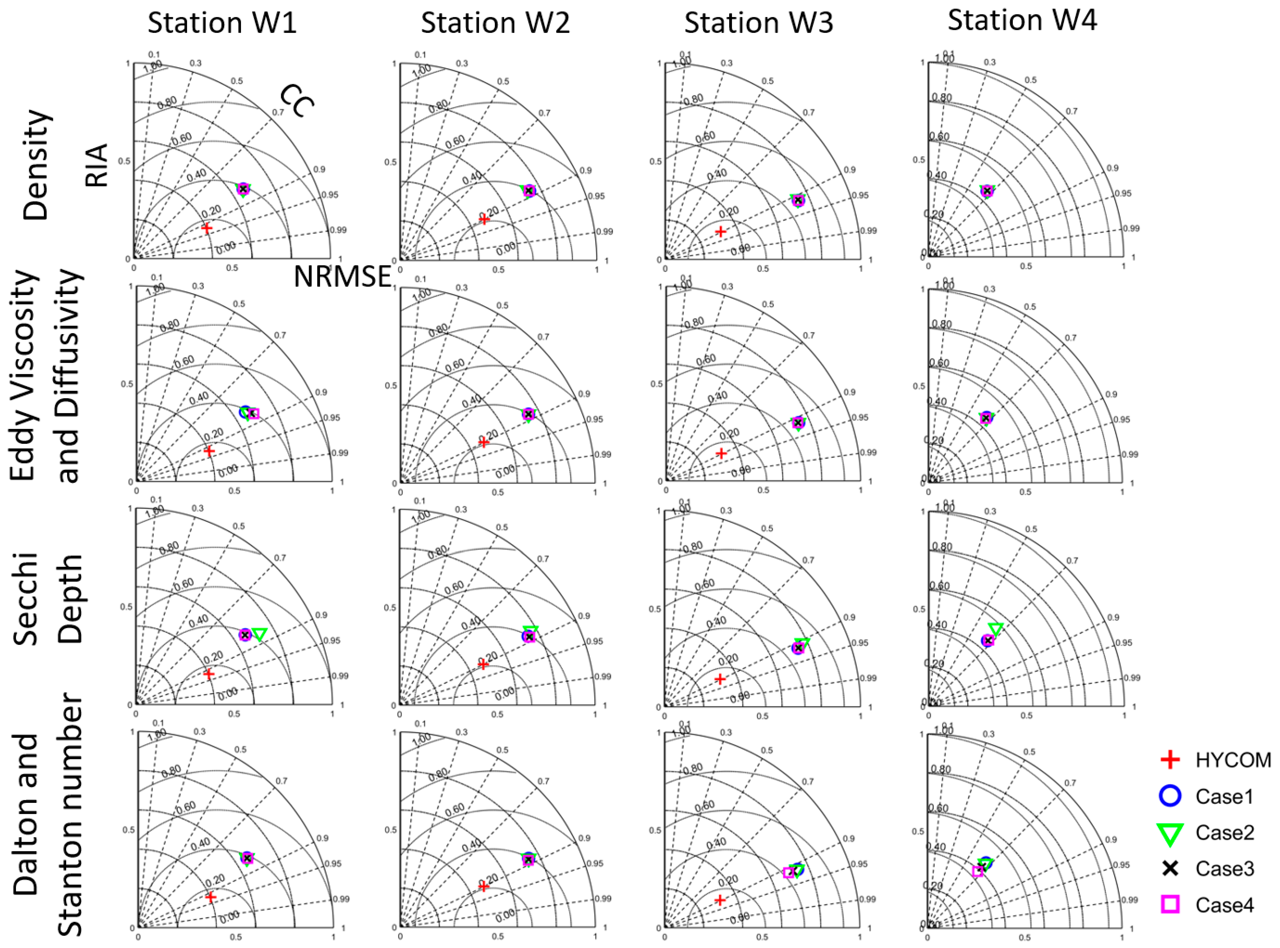
Figure 4.
Taylor diagram for error statistics of vertical profiles of salinity and temperature. Cases refer to Table 2. The locations of profiles P1 and P2 are in Figure 1.

Figure 5.
Comparisons of water level change during Hurricane Katrina in 2005: data (●) of NOAA stations and Delft3D model results (▬).
Figure 5.
Comparisons of water level change during Hurricane Katrina in 2005: data (●) of NOAA stations and Delft3D model results (▬).
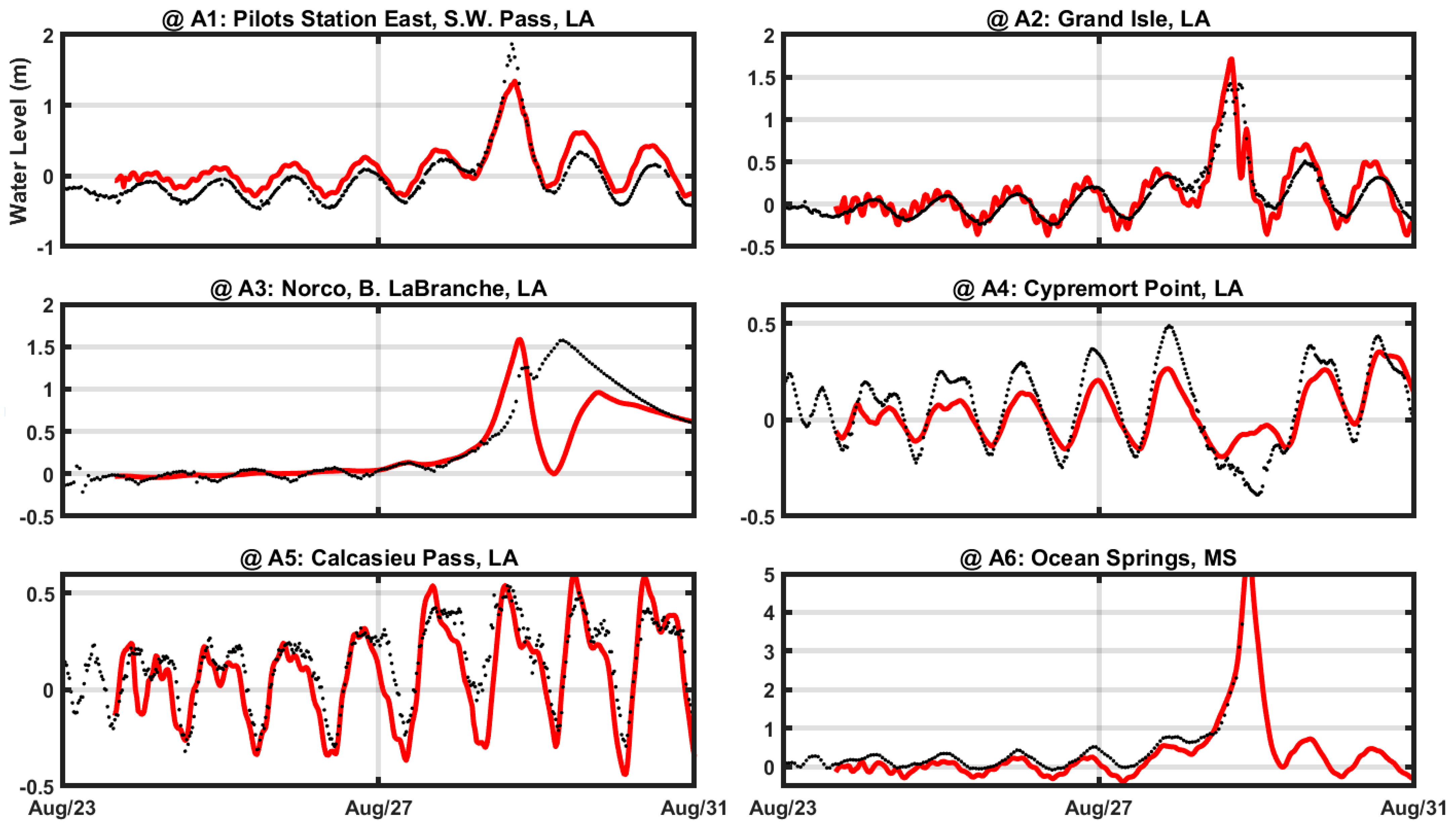
Figure 6.
Comparisons of wave (significant wave height and peak period) and wind (speed and direction) properties at NDBC stations. Data (●) and model results (▬).
Figure 6.
Comparisons of wave (significant wave height and peak period) and wind (speed and direction) properties at NDBC stations. Data (●) and model results (▬).
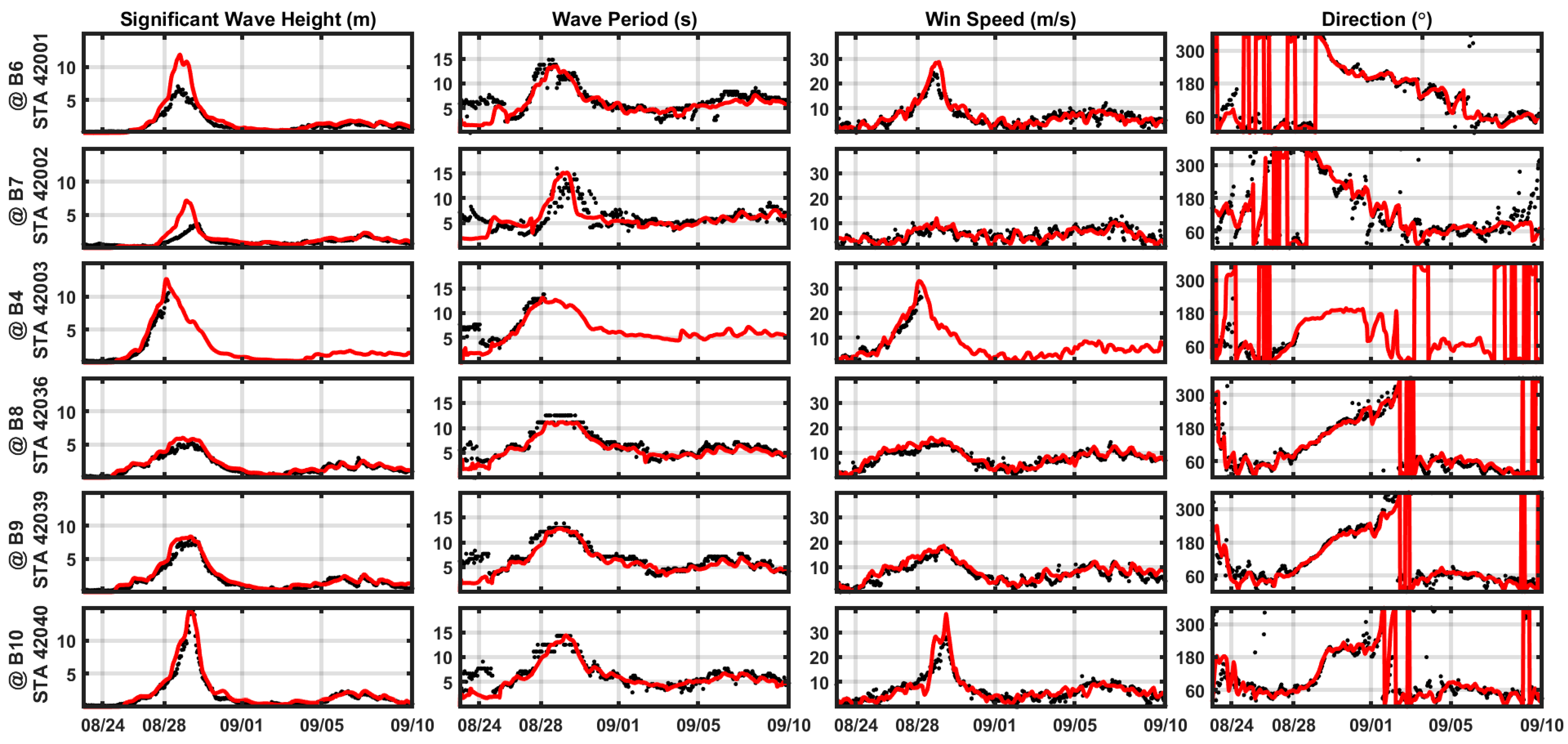
Figure 7.
Comparisons of vertical profiles of salinity and temperature on 10 July and 19 July: Profiles (● in black), HYCOM (♦ in blue), model results (★ in red).
Figure 7.
Comparisons of vertical profiles of salinity and temperature on 10 July and 19 July: Profiles (● in black), HYCOM (♦ in blue), model results (★ in red).

Figure 8.
Comparisons of 1–day mean water level (from the model) and altimeter sea surface height anomaly (from the TOPEX and ERS–2 satellites). The scatterplots are from pointwise comparisons between both data: the dashed-black line is the slope (linear fit), and correlation coefficients (CCs) were estimated for each time span.
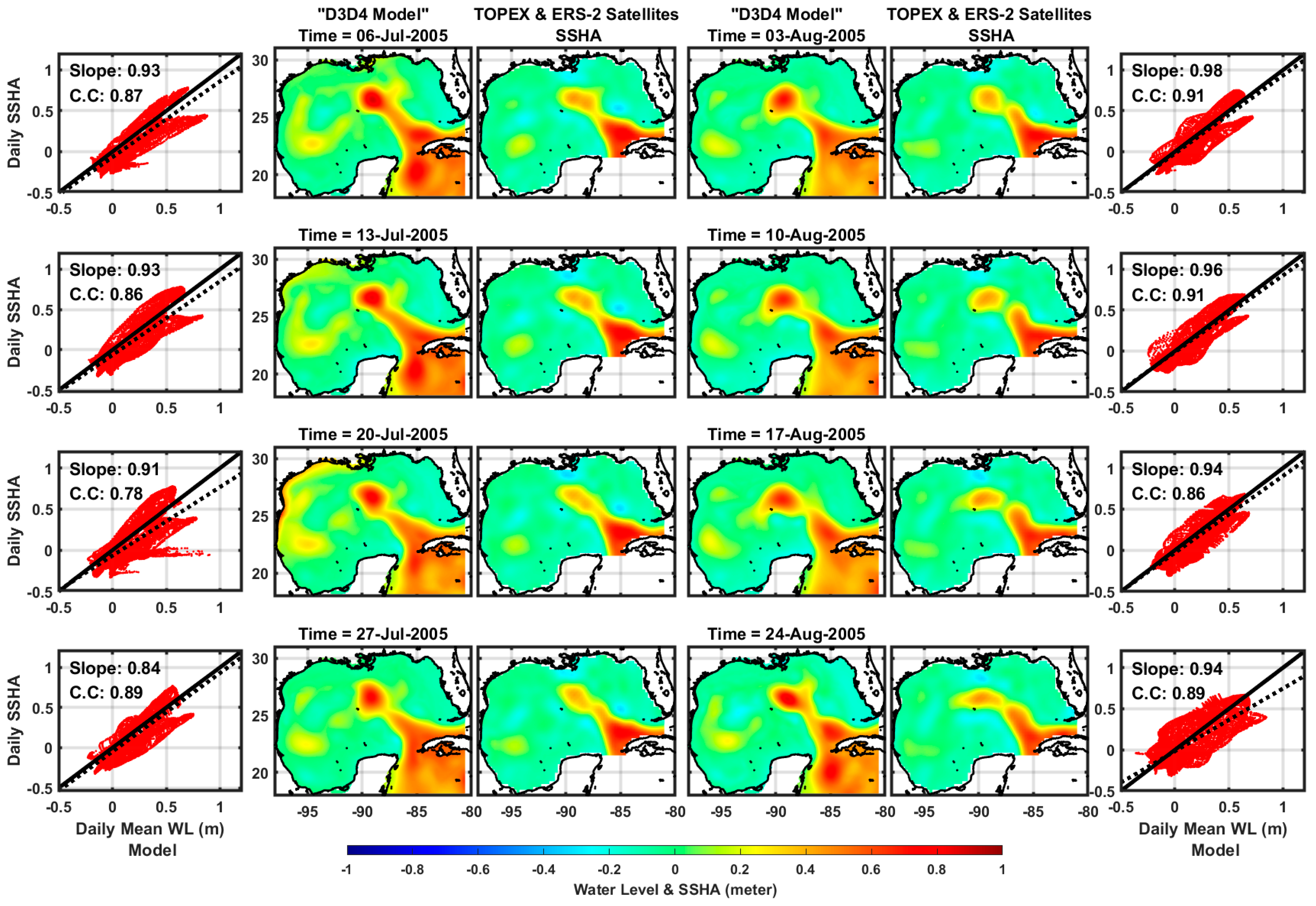
Figure 9.
Differences of vertical cross–sections (along the black dashed lines) of temperature (°C) and salinity (ppt) along the lines; left side, center and right side of the storm’s eye. The direction of the path is indicated as A to B.
Figure 9.
Differences of vertical cross–sections (along the black dashed lines) of temperature (°C) and salinity (ppt) along the lines; left side, center and right side of the storm’s eye. The direction of the path is indicated as A to B.
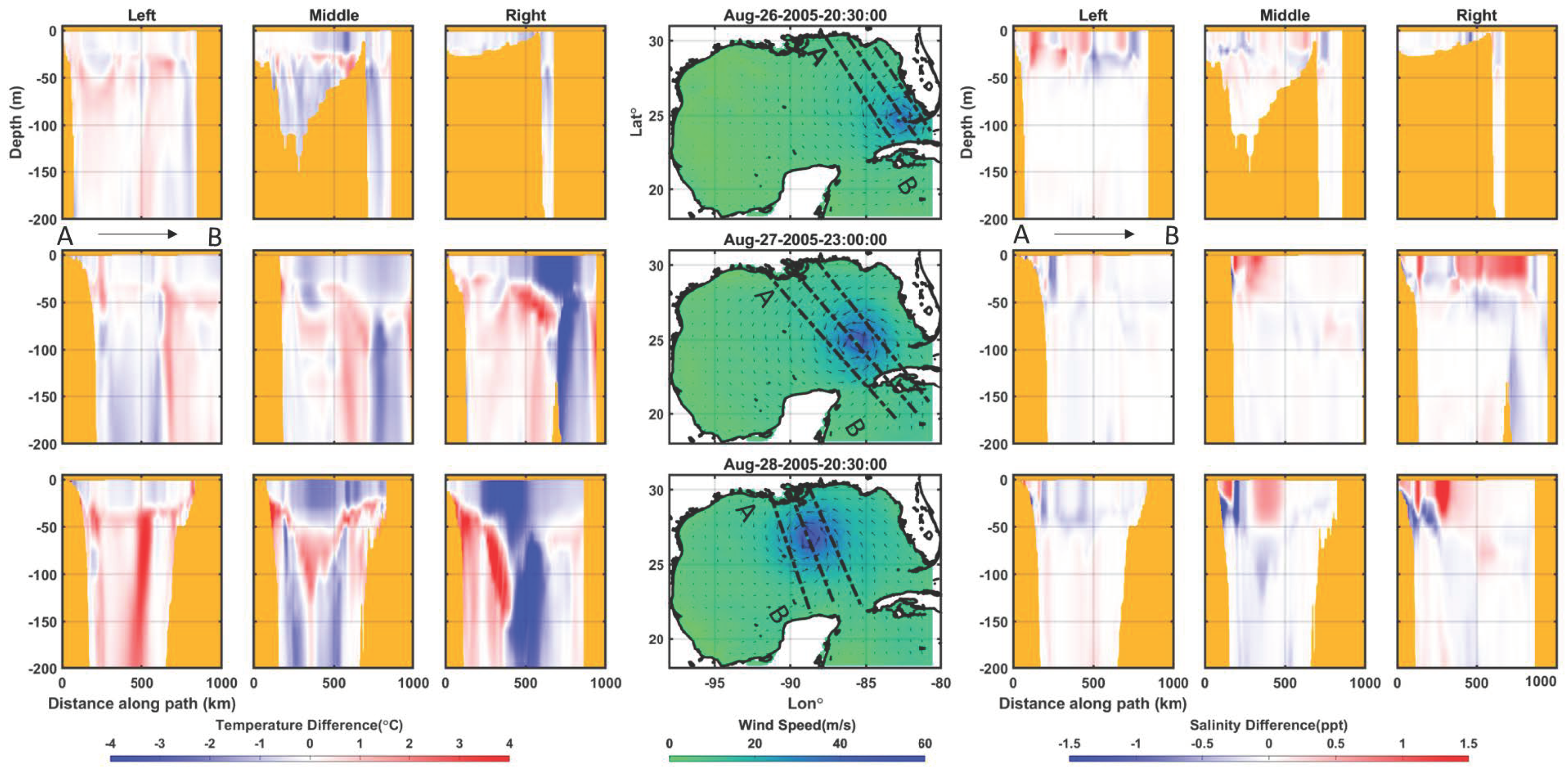
Figure 10.
Differences of vertical cross–sections (along the black dashed lines) of temperature (°C) and salinity (ppt) along the lines; upper, middle and lower portions of the storm’s eye. The direction of the path is indicated as A to B.
Figure 10.
Differences of vertical cross–sections (along the black dashed lines) of temperature (°C) and salinity (ppt) along the lines; upper, middle and lower portions of the storm’s eye. The direction of the path is indicated as A to B.

Figure 11.
Estimated daily mean mixed layer depths (MLDs, m, a2–h2) and wind fields (WSs, m/s, a1–h1) of Hurricane Katrina, ranging between 26 August and 1 September. Reference sea state and winds are averaged MLDs and WSs during 21–23 August, respectively. (a) average wind speed and MLD during August 21–23, wind speed and MLD on (b) August 26 12:00, (c) August 27 12:00, (d) August 28 12:00, (e) August 29 12:00, (f) August 30 12:00, (g) August 31 12:00, (h) September 01 12:00.
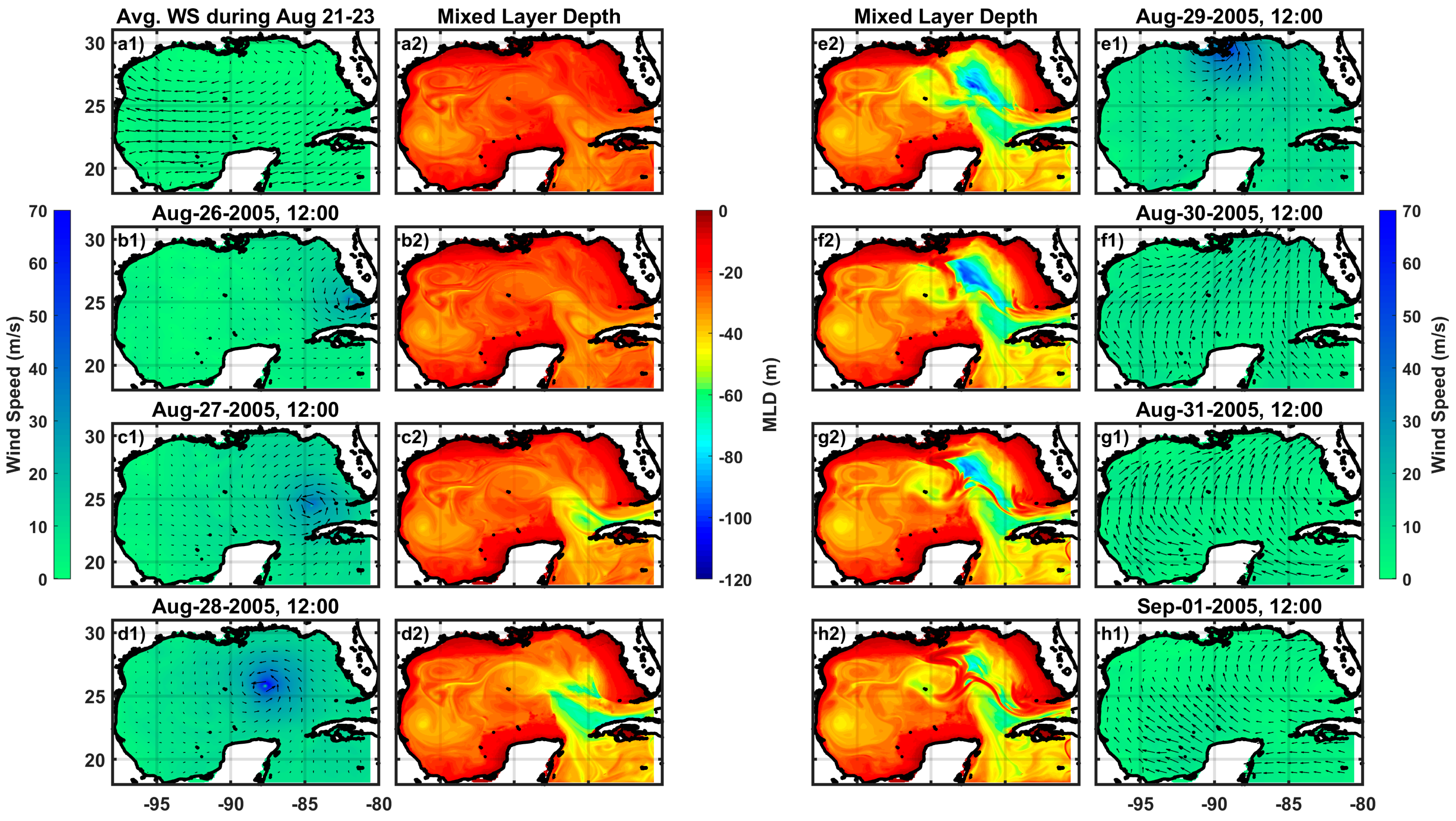
Figure 12.
(a) MLD recovery (%) from July in the Gulf of Mexico before Hurricane Katrina compared with mean MLD during 1–3 July; (b) MLD recovery from Hurricane Katrina compared with mean MLD during 1–3 July (►) and 21–23 August (●).
Figure 12.
(a) MLD recovery (%) from July in the Gulf of Mexico before Hurricane Katrina compared with mean MLD during 1–3 July; (b) MLD recovery from Hurricane Katrina compared with mean MLD during 1–3 July (►) and 21–23 August (●).

Figure 13.
Variations in MLD during Hurricane Katrina: (1) wind–field, (2) MLD in FLOW model, (3) MLD in coupled FLOW+WAVE model, (4) wave length along the line, (5) comparison of MLD along the black dashed line: FLOW (+) and FLOW+WAVE (▬).
Figure 13.
Variations in MLD during Hurricane Katrina: (1) wind–field, (2) MLD in FLOW model, (3) MLD in coupled FLOW+WAVE model, (4) wave length along the line, (5) comparison of MLD along the black dashed line: FLOW (+) and FLOW+WAVE (▬).
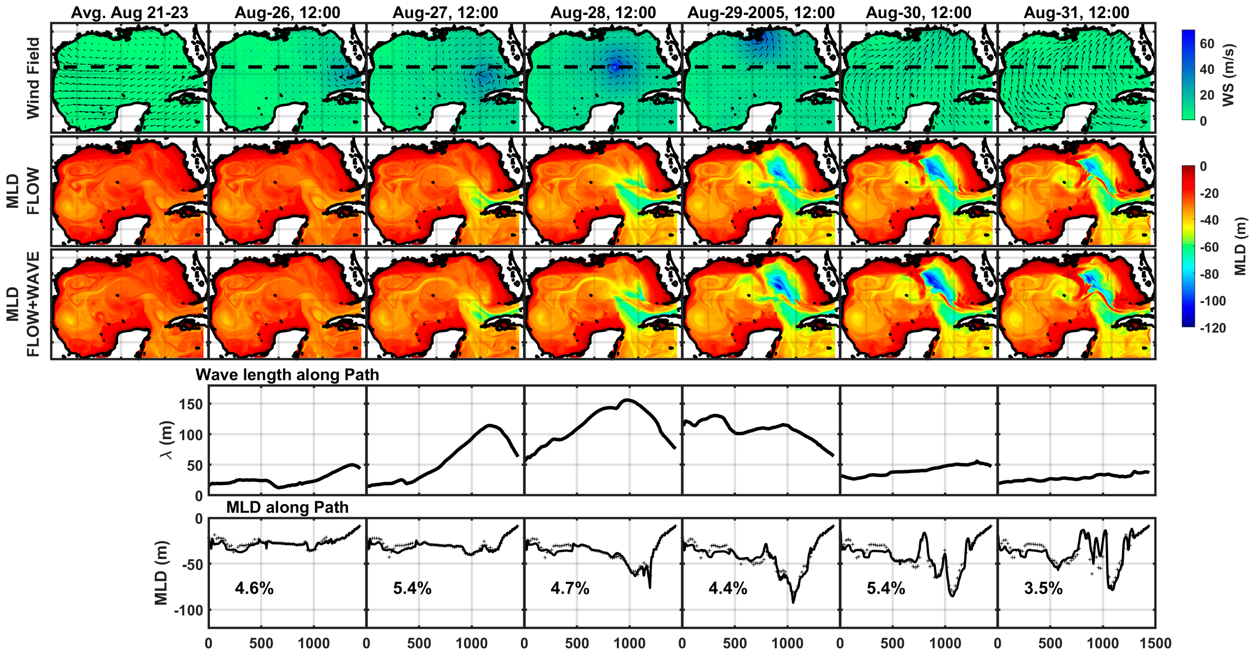
Figure 14.
Wave effects on the vertical cross–sections (along the black dashed lines) of temperature (°C) and salinity (ppt) along the lines; left side, center and right side of the storm’s eye. The direction of the path is indicated as A to B.
Figure 14.
Wave effects on the vertical cross–sections (along the black dashed lines) of temperature (°C) and salinity (ppt) along the lines; left side, center and right side of the storm’s eye. The direction of the path is indicated as A to B.
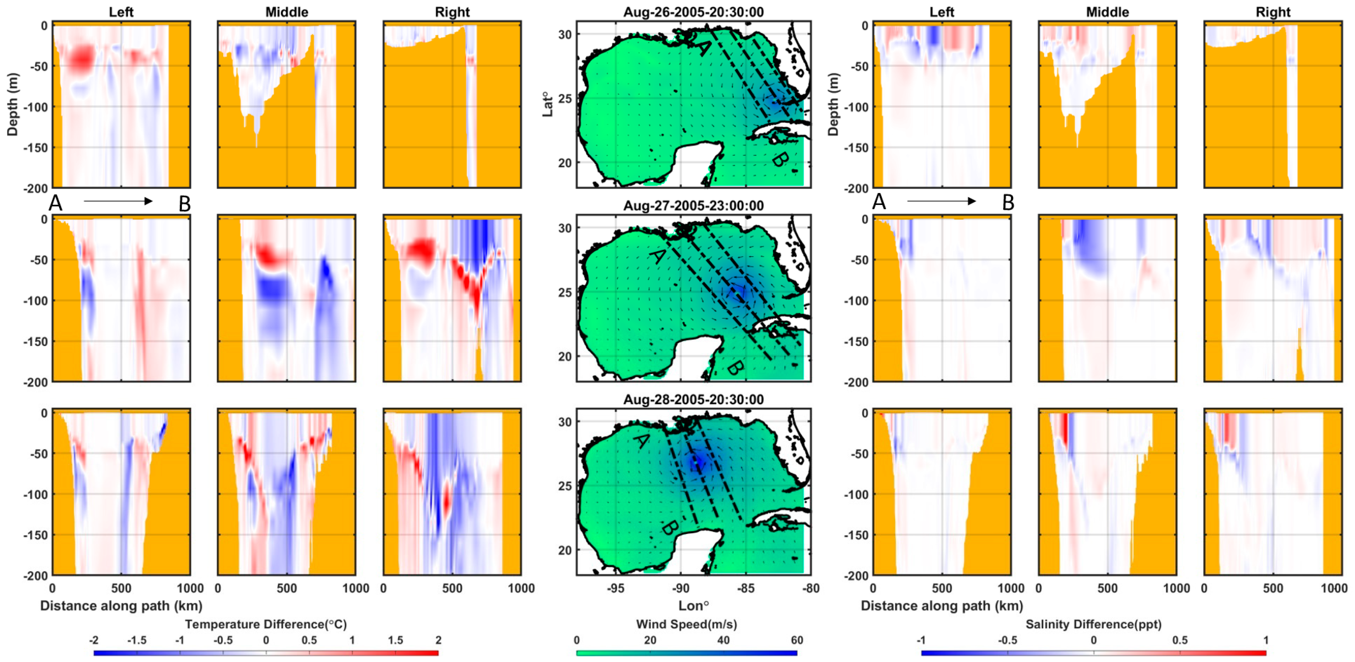
Figure 15.
Wave effects on the vertical cross–sections (along the black dashed lines) of temperature (°C) and salinity (ppt) along the lines; upper, middle, and lower portions of the storm’s eye. The direction of the path is indicated as A to B.
Figure 15.
Wave effects on the vertical cross–sections (along the black dashed lines) of temperature (°C) and salinity (ppt) along the lines; upper, middle, and lower portions of the storm’s eye. The direction of the path is indicated as A to B.


Table 1.
The physical parameters used in Delft3D modeling system.
| Dalton | 0.0041 |
| Stanton | 0.0041 |
| Air Density | 1.15 kg/m3 |
| Bottom Roughness | Manning’s Formula |
| Water: 0.02, Land: 0.08 | |
| Secchi Depth | 15 m |
| Background Horizontal | |
| Viscosity | 10 m2/s |
| Diffusivity | 10 m2/s |
Table 2.
A summary of physical parameters in the calibration process.
| Parameter | Value 1 | Value 2 | Value 3 | Value 4 |
|---|---|---|---|---|
| Eddy Viscosity/Diffusivity (m2/s) | 01/01 | 05/05 | 10/10 | 15/15 |
| Secchi Depth (m) | 3.5 | 5.0 | 10.0 | 15.0 |
| Dalton and Stanton Number | 0.0013/0.0013 | 0.0014/0.0014 | 0.0041/0.0041 | 0.0098/0.0098 |
Table 3.
Information of NOAA stations and profiles and statistical results of model validation during 1 July–1 September 2005.
Table 3.
Information of NOAA stations and profiles and statistical results of model validation during 1 July–1 September 2005.
| Lat | Lon | Parameter | RMSE | CC | RIA | |
|---|---|---|---|---|---|---|
| NOAA Stations (water level from mean sea level) | ||||||
| Corpus Christi, TX | 27.58 | −97.22 | Water level | 0.085 | 0.942 | 0.818 |
| Freeport, TX | 28.95 | −95.32 | ʺ | 0.081 | 0.942 | 0.831 |
| Calcasieu, LA | 29.77 | −93.35 | ʺ | 0.114 | 0.921 | 0.768 |
| Grand Isle, LA | 29.27 | −89.95 | ʺ | 0.118 | 0.855 | 0.643 |
| S.W Pass, LA | 28.93 | −89.40 | ʺ | 0.196 | 0.806 | 0.368 |
| Wave Land, MS | 30.28 | −89.37 | ʺ | 0.138 | 0.922 | 0.671 |
| Ocean Springs, MS | 30.40 | −88.80 | ʺ | 0.187 | 0.914 | 0.573 |
| Apalachicola, FL | 29.73 | −84.98 | ʺ | 0.267 | 0.848 | 0.321 |
| Tampa, FL | 27.87 | −82.55 | ʺ | 0.229 | 0.877 | 0.543 |
| Profiles (vertical structure of salinity and temperature) | ||||||
| Profile on 10 July | 27.79 | −86.20 | Salinity/Temperature | 0.18/0.85 | 0.999/0.999 | 0.89/0.92 |
| Profile on 19 July | 28.01 | −86.28 | ʺ | 0.26/0.69 | 0.926/0.996 | 0.89/0.92 |
Disclaimer/Publisher’s Note: The statements, opinions and data contained in all publications are solely those of the individual author(s) and contributor(s) and not of MDPI and/or the editor(s). MDPI and/or the editor(s) disclaim responsibility for any injury to people or property resulting from any ideas, methods, instructions or products referred to in the content. |
© 2024 by the authors. Licensee MDPI, Basel, Switzerland. This article is an open access article distributed under the terms and conditions of the Creative Commons Attribution (CC BY) license (https://creativecommons.org/licenses/by/4.0/).
Share and Cite
MDPI and ACS Style
Lee, W.; Veeramony, J. The Response of Mixed Layer Depth Due to Hurricane Katrina (2005). J. Mar. Sci. Eng. 2024, 12, 678. https://doi.org/10.3390/jmse12040678
AMA Style
Lee W, Veeramony J. The Response of Mixed Layer Depth Due to Hurricane Katrina (2005). Journal of Marine Science and Engineering. 2024; 12(4):678. https://doi.org/10.3390/jmse12040678
Chicago/Turabian StyleLee, Wonhyun, and Jayaram Veeramony. 2024. "The Response of Mixed Layer Depth Due to Hurricane Katrina (2005)" Journal of Marine Science and Engineering 12, no. 4: 678. https://doi.org/10.3390/jmse12040678
Note that from the first issue of 2016, this journal uses article numbers instead of page numbers. See further details here.