Effluent Mixing Modeling for Liquefied Natural Gas Outfalls in a Coastal Ecosystem

Abstract

Liquid Natural Gas (LNG) processing facilities typically are located on ocean shores for easy transport of LNG by marine vessels. These plants use large quantities of water for various process streams. The combined wastewater effluents from the LNG plants are discharged to the coastal and marine environments typically through submarine outfalls. Proper disposal of effluents from an LNG plant is essential to retain local and regional environmental values and to ensure regulatory and permit compliance for industrial effluents. Typical outfall designs involve multi-port diffuser systems where the design forms a part of the overall environmental impact assessment for the plant. The design approach needs to ensure that both near-field plume dispersion and far-field effluent circulation meets the specified mixing zone criteria. This paper describes typical wastewater process streams from an LNG plant and presents a diffuser system design case study (for an undisclosed project location) in a meso-tidal coast to meet the effluent mixing zone criteria. The outfall is located in a coastal and marine ecosystem where the large tidal range and persistent surface wind govern conditions for the diffuser design. Physical environmental attributes and permit compliance criteria are discussed in a generic format. The paper describes the design approach, conceptualization of numerical model schemes for near- and far-field effluent mixing zones, and the selected diffuser design.

1. Introduction

Total global demand for liquefied natural gas (LNG), which is one of the cleanest fossil fuels, is estimated to have grown by approximately seven percent per year since 2000 [1,2]. Driven by national environmental preference for lower carbon fuels, economic impacts of carbon emission costs and low shale gas prices, desire to diversify energy supply sources, geopolitics, and heightened popular opposition to post-Fukushima nuclear energy, the LNG production capacity is set to experience unprecedented growth by 2018 [2,3]. The number of new construction and operation of LNG plants also heightened environmental awareness in the plant permitting process. The LNG is primarily composed of methane, CH₄, which is converted to a liquid form for adequate storage and transport. In a typical LNG process the natural gas is first extracted from a deep on- or offshore gas exploration site, pre-treated and transported to an onshore or near shore processing plant where it is purified by removing condensates such as water, oil, mud, and other gases. An LNG process train would also typically be designed to remove trace amounts of mercury from the gas stream. The gas is then cooled down in stages until it is liquefied at approximately −260 °F at atmospheric pressure [4].

The LNG processing plants use large quantities of water for various process and wastewater streams. Plant wastewater is treated to meet required regulatory standards before wastewater effluents are discharged to the coastal and marine environments. Onshore LNG plants also support desalination of seawater to meet the large water demand of the LNG process and potable use during construction and operation of the LNG plant. Proper disposal of effluents from an LNG facility is essential to retain regional environmental values and ensure regulatory and permit compliance. The combined wastewater effluents are discharged through appropriately designed outfalls that commonly adopt a multi-port diffuser system in sufficiently deep waters. The diffuser system design accounts for the mixing characteristics in the near field and far field regions and generally forms a part of the plant overall environmental impact assessment.

In this paper, a diffuser system design case study is presented to meet the regulatory effluent mixing zone criteria. Although the project location is not specified, it is located on a meso-tidal coast with frequent storm surge impacts. The outfall is located in a coastal and marine ecosystem where large tidal range and persistent surface wind govern conditions for the diffuser design. Physical environmental attributes and permit compliance criteria for the case study are discussed in a generic format. The paper describes major LNG process wastewater streams, the diffuser system design approach, conceptualization of numerical model schemes for near- and far-field effluent mixing zones, and the selected diffuser design with particular emphasis on the modeling of the near-field mixing process.

2. LNG Process and Outfall Wastewater Streams

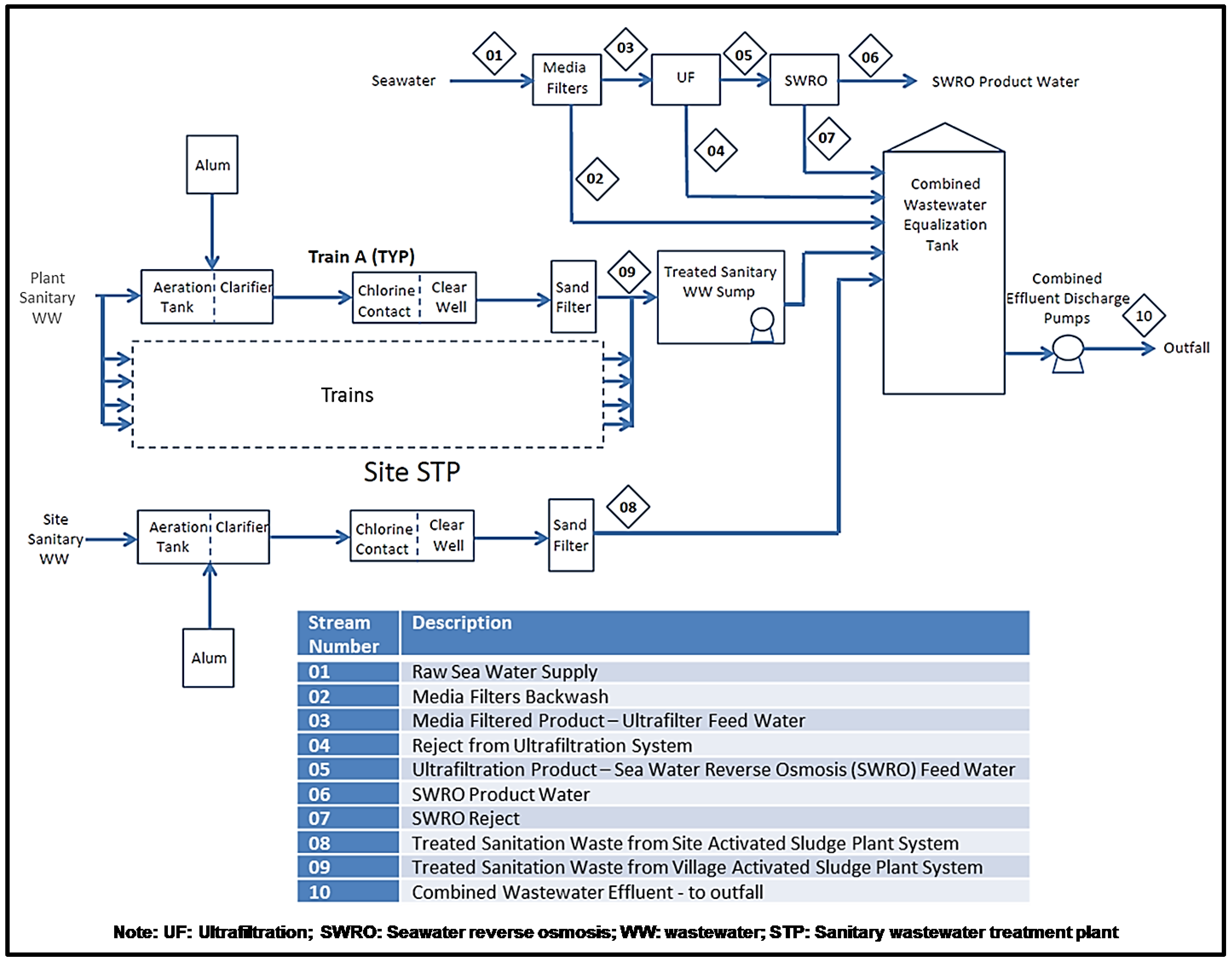
Onshore LNG plants support desalination of seawater to meet the large water demand of the LNG process and potable use during construction and operation of the LNG plant. Treated effluents from LNG plants may include several wastewater streams, for example, desalination plant brines, treated wastewater from LNG process streams, and treated sanitary wastewater.

Figure 1 shows a typical schematic description of the LNG plant wastewater process streams including outfall to natural environment. The figure shows one desalination (seawater reverse osmosis, SWRO) plant to supply SWRO product water to the LNG plant and SWRO filtration water and brines as wastewater to the equalizer tank. Treated wastewater from two sanitary wastewater streams, one from the LNG train areas and other from site facilities, are also pumped to the same equalizer tank. The final treated wastewaters from these streams are equalized in the combined equalizer tank before discharging to the outfall. The projected combined effluent flow rate from this system is estimated as approximately 750 m³/h.

Figure 1. Schematics of a typical LNG plant wastewater process streams.

Figure 1. Schematics of a typical LNG plant wastewater process streams.

3. Effluent Diffuser Design Approach

Environmental impacts from wastewater discharges are often evaluated based on the characteristics of effluent outfall plumes including mixing, dispersion and dilution, and ambient hydraulic characteristics such as currents, winds, temperature and density. Detailed evaluation of effluent outfall plumes is also important for meeting regulatory mixing zone criteria. Such effluent evaluation studies are performed employing numerical models that account for diffuser system design and resolve flow dynamics for the near field and far field regions. The near field region is characterized by small scales near the discharge location where flows are governed by diffuser designs, discharge properties and strong turbulent and jet mixing. On the other hand, the far field region is defined by large scales in the ambient receiving water where buoyant spreading motions and passive diffusion governs effluent dilution. Combination of these models is routinely used for mixing zone evaluation and wastewater disposal designs [5,6,7,8]. Several models are available for each flow types (near- and far-fields) focusing on the specific scales, resolutions and processes for each flow fields [9,10,11,12]. Plume models, which provide average plume characteristics in the near field zone, use spatial and temporal averaging of the flow field using equivalent diffuser characteristics. Consequently, the plume models simplify the processes using empirical techniques and analytical solutions based on the simplified geometry [9,10,13,14]. Hydrodynamic circulation models resolves the flow, density and temperature fields in three-dimensions solving the unsteady, baroclinic, shallow water equations [15,16].

In addition models that combine the near-field and far-field mixing processes are also proposed [17,18] to dynamically couple information exchanges between the models of varying time and space scales. Numerical fluid dynamic simulations, which are computationally very demanding, have also been performed to resolve the mixing process [19].

Present study uses a combination of near- and far-field models to evaluate outfall discharge configuration and mixing zone behavior. This paper presents results from both near- and far-field analyses with particular emphasis on the near-field mixing process. Effluent near-field mixing is evaluated by employing the Cornell Mixing Zone Expert System (CORMIX) modeling tool [9,10,13,14]. CORMIX is a steady-state mixing zone model for single or multi-port discharges particularly suitable for near-field mixing. CORMIX has the capability to analyse negatively buoyant effluents such as effluents from desalination plants that have higher density than the receiving water body. This is simulated in CORMIX such that the effluent flow from a submerged discharge port provides a velocity discontinuity between the discharged fluid and the ambient fluid causing an intense shearing action which breaks down into turbulent motion. This turbulent intensity progresses in the direction of the flow by entraining more of the ambient less turbulent fluid [9].

The far-field effluent mixing process is studied using the three-dimensional numerical model, Delft3D-FLOW [15]. The study investigates the far-field dispersion of the outfall discharge, the potentials for re-circulation of the effluent discharge as well as the dredged bathymetry impact on the extent of the mixing zone. Delft3D-FLOW is a three-dimensional hydrodynamic and transport process model, which simulates unsteady flow and transport phenomena that result from tidal and meteorological forcing. Delft3D-FLOW solves the governing flow equations for an incompressible fluid, under the shallow water assumptions and solves the equations on a rectilinear or a curvilinear boundary fitted grid system. The far-field model primarily was used to confirm the selected diffuser design from the near-field model.

4. Model Setup

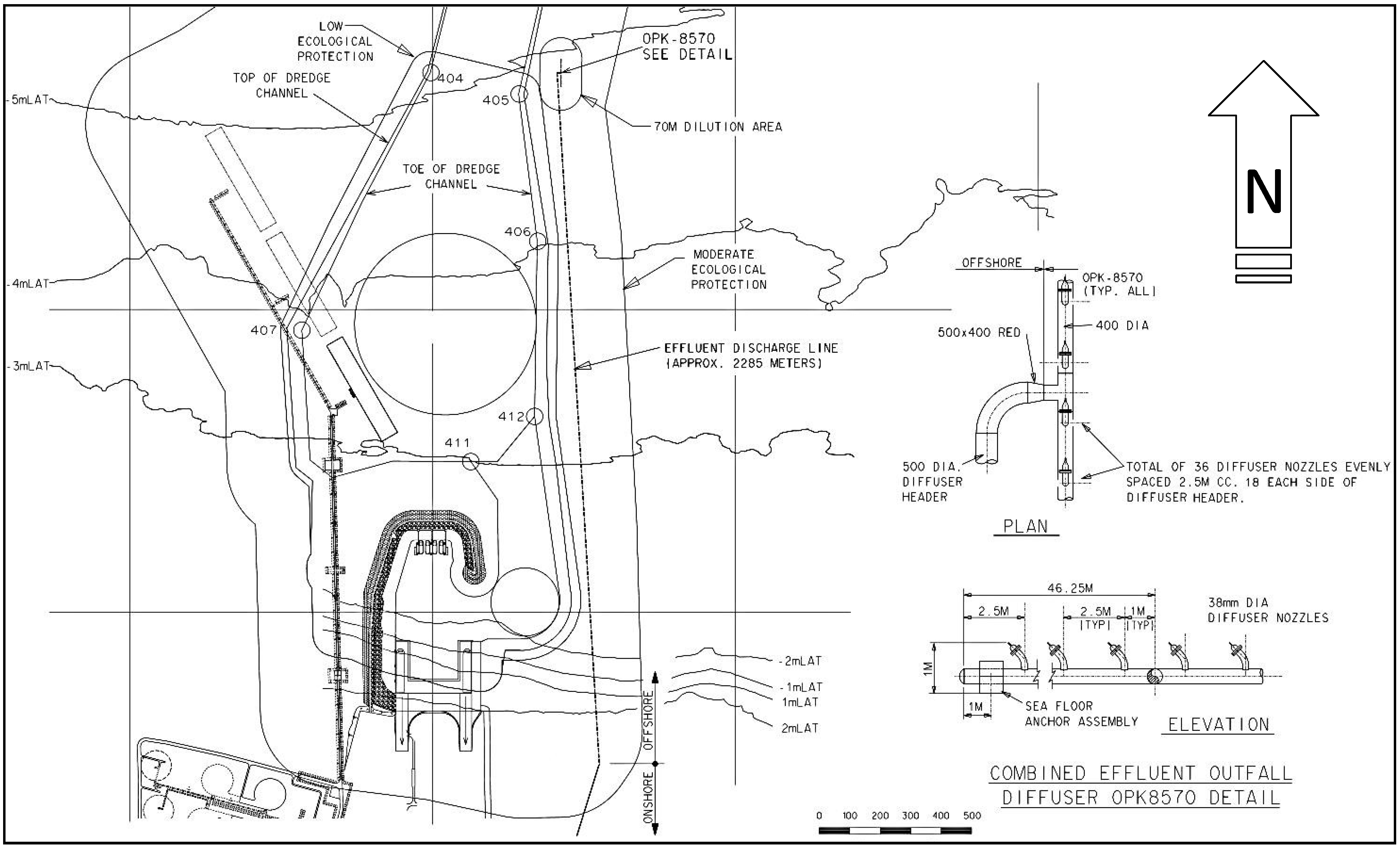
The shoreline and layout of the proposed outfall is shown in Figure 2. The outfall is located approximately 2.2 km from the shoreline at water depth of 5 m with respect to the lowest astronomical tide (LAT). For this analysis tidal water level variation is considered and the corresponding water depth and current velocity are used for each studied tidal conditions.

Figure 2. Outfall diffuser location and receiving water body.

Figure 2. Outfall diffuser location and receiving water body.

4.1. Physical Environment

Ambient conditions of the receiving water body of the coastal environment where the effluent discharges are described below.

4.1.1. Bathymetry

The bathymetry input comprises of bathymetry data (below water surface) and topography data (above water surface) from several data sources. A navigation channel is planned at the project site with a water depth of approximately 14.8 m relative to mean sea level (MSL). Figure 3 shows the pre-development bathymetry of the area. The diffuser system would be placed approximately at elevation 5 m below the lowest astronomical tide (LAT) (see Figure 2), which is considered as the uniform bottom elevation of the offshore-ward unbounded near-field model (CORMIX). The difference between MSL and LAT is approximately 1.5 m.

Figure 3. Bathymetry near the outfall location (depths are in meter relative to MSL).

Figure 3. Bathymetry near the outfall location (depths are in meter relative to MSL).

4.1.2. Wind Speed

Wind speeds of 3 m/s (breeze) were assumed in the direction towards the shore for the near-field simulation to represent a conservative design condition [8]. Although wind impacts are unimportant for near-field mixing [10], higher wind conditions likely would result in more dilution to the effluent plume.

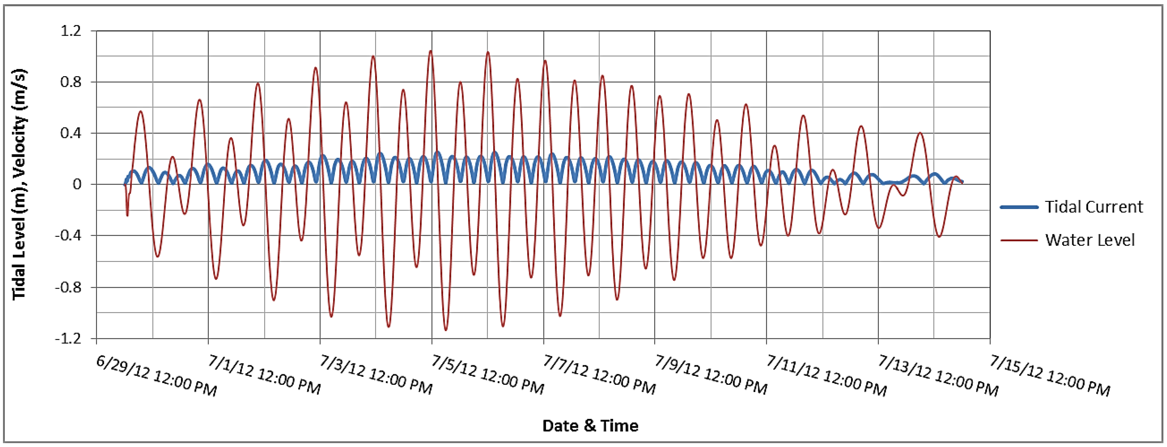
4.1.3. Tide

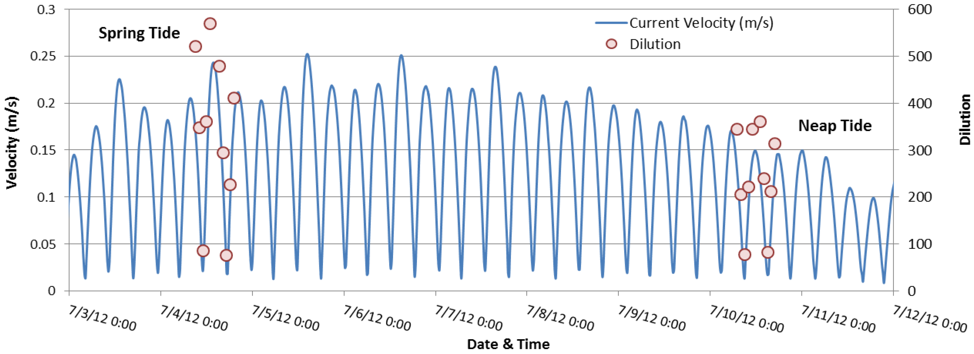
Figure 4 shows tidal water level and current variation over a neap-spring tidal cycle near the site. Note that all current magnitudes are presented as positive. As the outfall location experiences tidal reversals, near-field dilution analysis is performed at the tidal phase when current velocities are at or near slack tide. The following 20 tide phases were considered for the analysis:

• Four tidal conditions—high and low water slack under neap and spring tides.
• Five tidal phases—at slack tide, and one and two hours before and after slack tides.

4.1.4. Salinity, Temperature and Density

The average seawater salinity and temperature at the outfall area are 35 parts per thousand (ppt) and 25 °C (77 °F), respectively. No density stratification due to salinity is indicated for the coastal area near the outfall. The ambient density of the seawater was estimated based on the ambient total dissolved solids (TDS) concentration and temperature. Based on the methodology outlined in the UNESCO equation of state [20], TDS concentration of 37,600 mg/L (37.6 kg/m³) and temperature of 25 °C (77 °F), the seawater density is estimated as 1025.31 kg/m³.

4.1.5. Ambient Constituent Concentrations

The ambient TDS concentration of 37,600 mg/L corresponds to Stream Number 1, as shown in Figure 1, under maximum flow conditions. The ambient TSS (Total Suspended Solids) concentration was obtained as 5.3 mg/L corresponds to Stream Number 1 under average flow conditions. The ambient phosphorus concentration was obtained from measured data as 0.0135 mg/L, which was taken as a conservative value. The ambient nitrogen concentration was obtained as 0.15 mg/L corresponding to Stream Number 1. This value is estimated as an average of measured data close to the site.

Figure 4. Variation of tidal water level and current near the site over a neap-spring cycle.

Figure 4. Variation of tidal water level and current near the site over a neap-spring cycle.

4.2. Diffuser Geometry

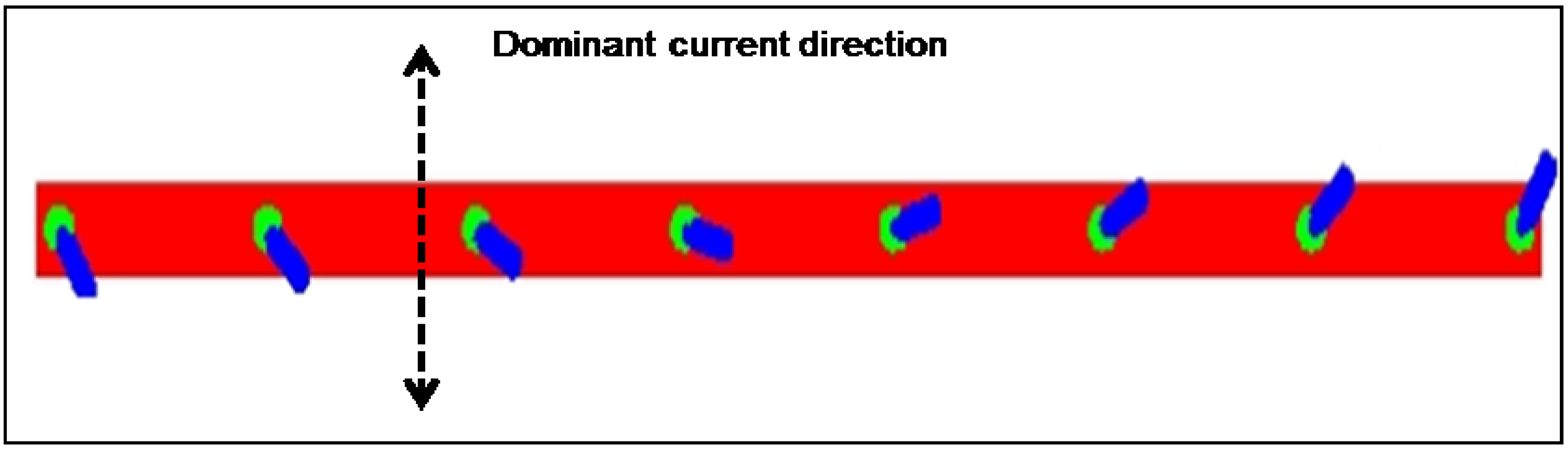
A Staged Fanned diffuser type of arrangement is selected to discharge the combined effluent to the marine environment. Sketch of the diffuser is given in Figure 5. The staged fanned type produces a net horizontal momentum flux parallel to the diffuser line and gave the maximum possible dilution when compared to other diffuser types.

Figure 5. Schematic of staged fan diffuser.

Figure 5. Schematic of staged fan diffuser.

The number of ports (36) was selected based on the duckbill exit velocity. For this analysis, the exit velocity was used to determine the number of ports based on the discharge rate of approximately 750 m³/h. The flow per nozzle is then calculated as total flow divided by the number of ports (36), which equals to about 21 m³/h. The staged fanned design type was selected to ensure adequate dilution is attained during different flow directions as well as eliminate any effluent plume hitting the surface. In CORMIX, the duckbill type check valves are modelled with steady flow effluent discharge at the design flow rate.

4.3. Effluent Discharge Conditions

For this analysis, the required dilution values for the following constituents were evaluated: TDS, Total Nitrogen (Ntot), Total Phosphorous (Ptot), Total Suspended Solids (TSS), and Aluminum (Al+).

Mixing Criteria

The criteria for effluent constituents are based on regulatory requirements at the edge of the defined mixing zone (70 m from the outfall location). The TDS and salinity values are typically correlated and the mixing zone criterion adopted was +5 percent of ambient for both. The criterion for TDS was then estimated as 39,480 mg/L (+5 percent of 37,600 mg/L). As the background concentrations of Ntot are above the regulatory guideline of 0.1 mg/L, the 80th percentile of the background concentrations was used as the site specific standard, which was estimate to be 0.187 mg/L. The Ptot, TSS and AL+ criteria were taken as 0.015 mg/L, 8 mg/L and 0.32 mg/L, respectively, following regulatory guidelines.

The geometric characteristics of the diffuser includes a diffuser length of 92.5 m with an orientation of 90° to current direction, 36 Duckbill valve type ports each with an area of 0.00082 m² with equivalent diameter of 0.03231 m at 45° vertical angle from horizontal. A spacing of 2.5 m between ports is assumed with the port height of 1.0 m above seabed. The seabed slope at the diffuser is assumed horizontal. Based on the flow rate (750 m³/h) and port opening (0.00082 m²), the exit velocity at the port/duckbill valve is 7.16 m/s.

4.4. Model Simulation Cases

Two cases of effluent composition are evaluated, as can be seen in Table 1. Case 1 represents effluent discharge condition with high TDS and Case 2 with low TDS magnitudes. The two cases represent various stages of the plant construction and operation to bind the expected range of effluent properties and expected environmental impacts. A number of CORMIX simulations were performed for the two cases to arrive at a suitable diffuser design meeting the following restrictions:

(a)

Sufficient effluent dilution is reached that would meet the required constituents’ concentrations at the end of the mixing zone as specified before.

(b)

The port vertical angle is 45° for ease of construction.

(c)

The diffuser type, orientation and alignment minimize any effluent plume hitting the water surface.

(d)

The diffuser design consistently meets the required dilution during tidal reversals and tide phases close to reversals at the outfall location and over the range of neap-spring tide cycle.

Table 1. Outfall discharge evaluation cases.

Parameters	Case 1	Case 2
Intake Seawater Flow Rate (m3/h)	966	0.0
Outfall Discharge Flow Rate (m3/h)	750	750
Total Dissolved Solids (TDS) (mg/L)	49,706	600
Total Nitrogen (Ntot) (mg/L)	6.8	35
Total Phosphorus (Ptot) (mg/L)	0.78	4
Total Suspended Solids (TSS) (mg/L)	24.2	10
Al+ (mg/L)	0.0	0.08

Table 1. Outfall discharge evaluation cases.

Parameters	Case 1	Case 2
Intake Seawater Flow Rate (m3/h)	966	0.0
Outfall Discharge Flow Rate (m3/h)	750	750
Total Dissolved Solids (TDS) (mg/L)	49,706	600
Total Nitrogen (Ntot) (mg/L)	6.8	35
Total Phosphorus (Ptot) (mg/L)	0.78	4
Total Suspended Solids (TSS) (mg/L)	24.2	10
Al+ (mg/L)	0.0	0.08

Slack tide is typically the most conservative conditions for dilution analysis as ambient velocity becomes at or near stagnation conditions producing the lowest dilutions.

5. Model Results

Table 2 shows the results of the near-field dilution simulation cases for the spring and neap tides for Case 1 and Case 2. The variation of dilution for various tidal phases for Case 1 is also shown in Figure 6 along with tidal currents. As can be seen from the table and the figure, dilution has a strong correlation with tidal current with higher current magnitude providing higher dilution. The lowest dilution can be observed at slack phases, which is only active for a short period of time. Based on the variation of dilution over the tidal phases, the minimum dilution one hour after the slack tide over the neap-spring cycle for each case was selected for applying the mixing zone criteria.

Table 2. Results of dilution analysis.

Description	Tidal Phases	Current (m/s)	Dilution at the End of Mix Zone		Comments
			Case 1	Case 2
HW—Spring	2 h before slack	0.17	521	525
	1 h before slack	0.1	348	355
	Slack	0.02	85	84	At 81 m
	1 h after slack	0.13	360	365
	2 h after slack	0.22	570	575
LW—Spring	2 h before slack	0.19	479	483
	1 h before slack	0.12	294	302
	Slack	0.02	76	76	At 103 m
	1 h after slack	0.11	226	235
	2 h after slack	0.19	410	412
LW—Neap	2 h before slack	0.13	344	352
	1 h before slack	0.07	206	219
	Slack	0.01	78	78	At 94 m
	1 h after slack	0.09	221	230
	2 h after slack	0.14	345	353
HW—Neap	2 h before slack	0.12	360	368
	1 h before slack	0.07	239	249
	Slack	0.02	83	83	At 86 m
	1 h after slack	0.07	212	218	Selected dilution
	2 h after slack	0.13	344	352

Note: HW: High water; LW: Low water.

Table 2. Results of dilution analysis.

Description	Tidal Phases	Current (m/s)	Dilution at the End of Mix Zone		Comments
			Case 1	Case 2
HW—Spring	2 h before slack	0.17	521	525
	1 h before slack	0.1	348	355
	Slack	0.02	85	84	At 81 m
	1 h after slack	0.13	360	365
	2 h after slack	0.22	570	575
LW—Spring	2 h before slack	0.19	479	483
	1 h before slack	0.12	294	302
	Slack	0.02	76	76	At 103 m
	1 h after slack	0.11	226	235
	2 h after slack	0.19	410	412
LW—Neap	2 h before slack	0.13	344	352
	1 h before slack	0.07	206	219
	Slack	0.01	78	78	At 94 m
	1 h after slack	0.09	221	230
	2 h after slack	0.14	345	353
HW—Neap	2 h before slack	0.12	360	368
	1 h before slack	0.07	239	249
	Slack	0.02	83	83	At 86 m
	1 h after slack	0.07	212	218	Selected dilution
	2 h after slack	0.13	344	352

Note: HW: High water; LW: Low water.

The selected dilution for each case was then applied to calculate the equivalent effluent constituent concentrations at the end of the mixing zone for comparisons with the effluent criteria as in Table 3.

Figure 6. Variation of dilution over the spring-neap tidal cycle for Case 1.

Figure 6. Variation of dilution over the spring-neap tidal cycle for Case 1.

Table 3. Effluent constituent concentration at the end of mixing zone.

Constituent	Unit	Ambient	Effluent	Criteria	Case 1			Case 2
					Required Dilution	Selected Dilution	Conc.	Required Dilution	Selected Dilution	Conc.
TDS	mg/L	37,600	49,706	39,480	6	212	37,655	N/A	218	37,425
Ntot	mg/L	0.15	6.8	0.187	180		0.1804	942		0.3144
Ptot	mg/L	0.0135	0.78	0.015	511		0.017	2658		0.0323
TSS	mg/L	5.3	24.2	8	7		5.3863	2		5.3222
Al+	mg/L	0	0	0.32	0		-	0		0.0004

Note: The effluent TDS concentration for Case 2 is smaller than the ambient concentration.

Table 3. Effluent constituent concentration at the end of mixing zone.

Constituent	Unit	Ambient	Effluent	Criteria	Case 1			Case 2
					Required Dilution	Selected Dilution	Conc.	Required Dilution	Selected Dilution	Conc.
TDS	mg/L	37,600	49,706	39,480	6	212	37,655	N/A	218	37,425
Ntot	mg/L	0.15	6.8	0.187	180		0.1804	942		0.3144
Ptot	mg/L	0.0135	0.78	0.015	511		0.017	2658		0.0323
TSS	mg/L	5.3	24.2	8	7		5.3863	2		5.3222
Al+	mg/L	0	0	0.32	0		-	0		0.0004

Note: The effluent TDS concentration for Case 2 is smaller than the ambient concentration.

Discussion on Model Results

Model results for near-field simulations in Table 2 and Table 3 show that the criteria for all constituents are met except for Ptot in Case 1 and Ntot and Ptot for Case 2. With the current dilution factor for Case 1 and an ambient concentration of 0.01 mg/L, the Ptot effluent criteria could be met with an effluent concentration of 0.0135 mg/L. Ptot effluent concentration should not exceed 0.34 mg/L (instead of 0.78 mg/L) if the standard is to be met through the tidal signal. It should be noted that the criteria for Ptot could be met several hours from slack tide when stronger tidal currents exist in the outfall location.

For Ntot, the effluent criteria would be met in Case 1. However, for Case 2, the high effluent concentration (35 mg/L) would exceed the mixing zone criteria for some tidal phases. Ntot effluent concentration should not exceed 8 mg/L if the standard is to be met through the tidal cycle.

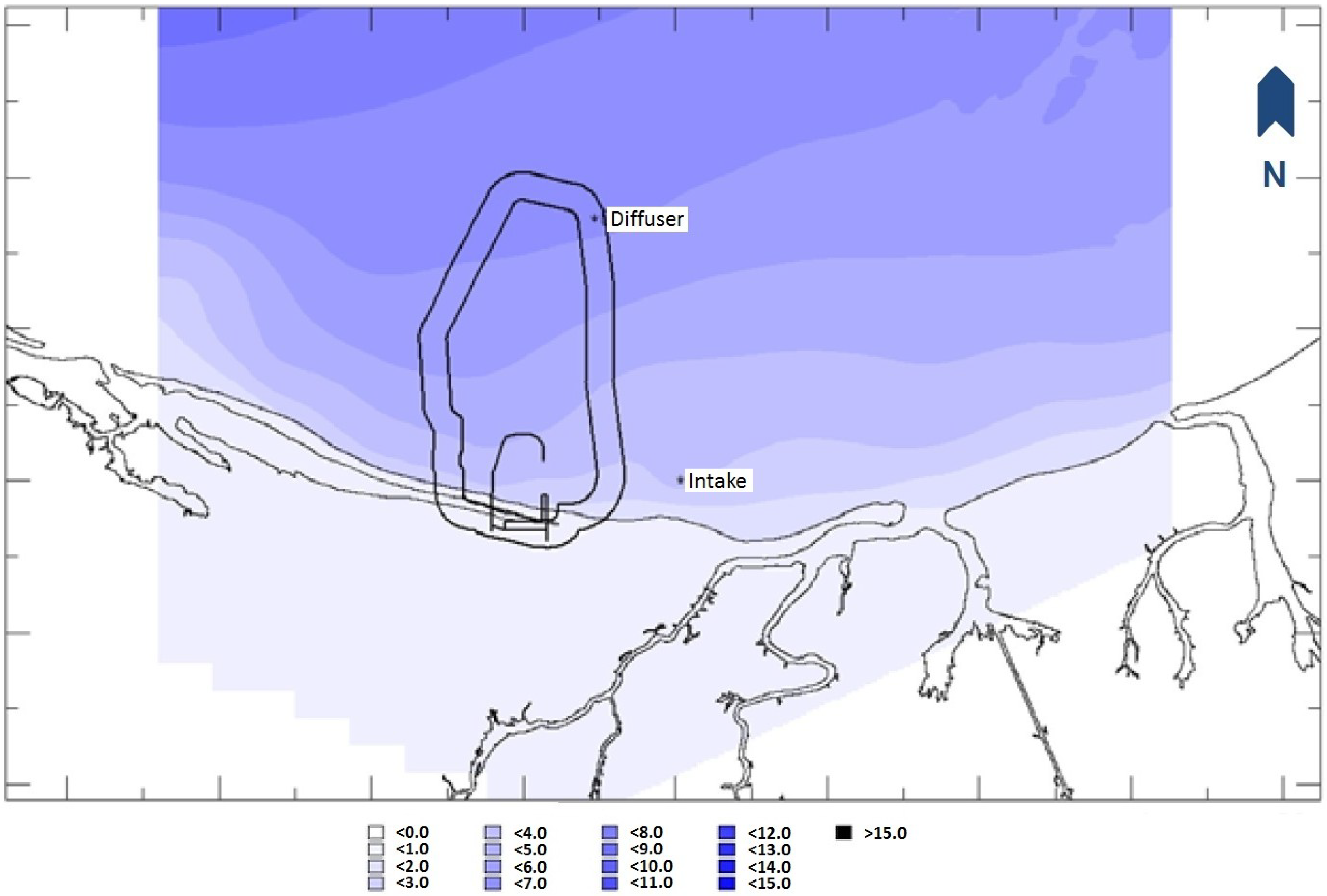
Delft3D model simulations were performed with CORMIX results as input to the model for design verification in the far field. The far-field Delft3D model employs a nested rectilinear grid model with horizontal grid spacing varying as 180 m, 60 m and 20 m. The fine mesh grid covers the diffuser region with the effluent concentrations from CORMIX lumped over one Delft3D grid to represent the near field mixing. A sigma grid vertical coordinate system is selected for the model with the coarse, medium and fine grid domains represented with 1, 3 and 6 layers, respectively. The model results show that, in general, the impact of the effluent discharge on the intake is insignificant for all cases considered. For the high TDS case, the dredged bathymetry appears to guide the effluent toward the intake area. The time-series of the TDS concentration shows above ambient at the intake area; however, the maximum above ambient concentration is shown to be far below the near-field criteria for the TDS constituent. As noted before, the far-field model only provides a confirmation of the near filed mixing analysis, which governed the diffuser design including the type, size and number of diffuser ports, port discharge angle and spacing.

It should be noted that the approach to combine the results of near field simulations into the far field model is not dynamic and treated as one-way offline input. Changes in ambient conditions as a result of the near field mixing after each tidal phase are not accounted for in the far field model. Also, quasi transient treatment of the tidal cycle in the near field model only to a limited extent accounts for the accumulation of constituent concentration during tidal reversal [10]. The design of the diffuser system therefore is dependent on the conservatively selected dilution factor in the near-field model. Also, after each tidal phase the near-field model did not update he ambient flow field from the far-field model results. Therefore, accumulation of concentration built-up during tidal reversal over several tidal cycles has not been accurately modeled in the in the near-field CORMIX model.

6. Conclusions

This paper describes typical wastewater process streams from an LNG plant and presents a diffuser system design case study in a meso-tidal coast to meet the effluent mixing zone criteria. CORMIX mixing model is employed to evaluate the near field mixing process of the combined plant effluent in marine environment. Three dimensional Delft3D model is used for the far field mixing only as a confirmatory analysis taking input from the near-field model. The neap-spring tidal cycle is discretized on a quasi-steady approach to evaluate dilution in the Cormix model. A staged fanned diffuser with 36 ports and 2.5 m spacing was used to achieve significant dilution within the mixing zone boundary. The length of the diffuser is 92.5 m.

The dilution factor at the boundary of the mixing zone was obtained by taken the lowest possible dilution around various slack tide conditions for neap and spring tides from the CORMIX simulations. The analysis showed that although not all effluent constituents would meet the regulatory mixing zone criteria for all tidal phases for the selected diffuser design and marine environment, the dilution criteria would be met for all constituents for most tidal phases. Also, the large tidal range and persistent surface wind govern the conditions for the diffuser design.

References

- Sankey, P.; Hermann, L.; Clark, D.T.; Micheloto, S.; Nip, W. Gorgon & the Global LNG Monster, Deutsche Bank Markets Research: Global LNG; Deutsche Bank Securities Inc.: New York, NY, USA, 2012; p. 82. [Google Scholar]
- International Energy Agency. World Energy Outlook 2012. Available online: http://www.worldenergyoutlook.org/pressmedia/recentpresentations/PresentationWEO2012launch.pdf (accessed on 12 December 2013).
- Morgan Cazanove, J.P. Global LNG: Full Steam Ahead, but Cross-basin Arbitrageurs beware Henry Hub Price Diffusion; Global Equity Research, J.P. Morgan Chase & Co.: London, UK, 2012; p. 248. [Google Scholar]
- LNG Technology Licensing, ConocoPhilips: Liquefied Natural Gas. Available online: http://lnglicensing.conocophillips.com/EN/Pages/index.aspx (accessed on 13 December 2013).
- Doneker, R.L.; Ramachandran, A.; Opila, F. CORMIX modeling of sediment plumes for the oil and gas industry. In Proceedings of the International Symposium on Outfall Systems, Mar del Plata, Argentina, 15–18 May 2011.
- Chopakatla, S.; Khangaonkar, T.; Sorenson, T. A detailed study of the zone of initial dilution to evaluate exposure and fish entrainment—Fort James operating company’s Wauna outfall. In Proceedings of the Engineering, Pulping and Environmental Conference, Atlanta, GA, USA, 5–8 November 2006; Curran Associates, Inc.: Red Hook, NY, USA, 2007; pp. 440–454. [Google Scholar]
- Maia, L.P.; Bezerra, M.O.; Pinheiro, L.; Redondo, J.M. Application of the Cormix model to assess environmental impact in the coastal area: An example of the ocean disposal system for sanitary sewers in the city of Fortaleza (Ceara, Brazil). J. Coast. Res. 2011, 64, 922–925. [Google Scholar]
- Nigam, S.; Rao, B.P.S.; Srivastava, A. Effect of thermal discharge of cool water outfall from liquefied natural gas (LNG) plant into sea using Cormix. J. Comput. Commun. Sci. Res. 2013, 1, 9–13. [Google Scholar] [CrossRef]
- Akar, P.J.; Jirka, G.H. Cormix2: An Expert System for Hydrodynamic Mixing Zone Analysis of Conventional and Toxic Multiport Diffuser Discharges; Technical Report EPA/600/3–91/073; U.S. Environmental Research Laboratory: Athens, Georgia, 1991. [Google Scholar]
- Jirka, G.H.; Doneker, R.L.; Hinton, S.W. User’s Manual for CORMIX: A Hydrodynamic Mixing Zone Model and Decision Support System for Pollutant Discharge into Surface Waters; U.S. Environmental Protection Agency: Ithaca, NY, USA, 1996; p. 152. [Google Scholar]
- Wood, I.R.; Bell, R.G.; Wilkinson, D.L. Ocean Disposal of Wasterwater. Advanced Series on Ocean Engineering—Volume 8; World Scientific: Singapore, 1993; p. 425. [Google Scholar]
- Fischer, H.B.; List, E.J.; Koh, R.C.Y.; Imberger, J.; Brooks, N.H. Mixing in Inland and Coastal Waters; Academic Press: Oxford, UK, 1979; p. 483. [Google Scholar]
- Doneker, R.L.; Jirka, G.H. CORMIX1: An Expert System for Mixing Zone Analysis of Conventional and Toxic Single Port Aquatic Discharges; U.S. EPA, Environmental Research Laboratory: Athens, GA, USA, 1990; EPA-600/600/3–90/012.
- Jirka, G.H. Use of mixing zone models in estuarine waste load allocation. In Part III of Technical Guidance Manual for Performing Waste Load Allocations, Book III: Estuaries; Ambrose, R.A., Discharges, J., Martin, J.L., Eds.; U.S. EPA: Washington, DC, USA, 1992; EPA-823-R-92–004. [Google Scholar]
- Deltares. Delft3D-FLOW, Simulation of Multi-Dimensional Hydrodynamic Flows and Transport Phenomena, including Sediments, User Manual, Version: 3.14, Revision: 9772, 4 December 2009; Deltares: Delft, The Netherland, 2009. [Google Scholar]
- Danish Hydraulic Institute. MIKE21 Flow Model: Hydrodynamic Module, Scientific Documentation; Danish Hydraulic Institute: Hørsholm, Denmark, 2010. [Google Scholar]
- Morelissen, R.; Kaaij, T.V.D; Bleninger, T. Waste water discharge modelling with dynamically coupled near field and far field models. In Proceedings of the International Symposium on Outfall Systems, Mar del Plata, Argentina, 15–18 May 2011.
- Choi, K.W.; LEE, J.H.W. A new approach to effluent plume modelling in the intermediate field. In Proceedings of the XXXI IAHR Congress, Seoul, Korea, 11–16 September 2005.
- De Wit, L. Near field 3D CFD modelling of overflow plumes. In Proceedings of the 19th World Dredging Conference (WODCON XIX), Beijing, China, 9–14 September 2010.
- UNESCO. Background Papers and Supporting Data on the International Equation of State of Seawater 1980; Technical Papers in Marine Science; UNESCO: Paris, France, 1981; p. 192. [Google Scholar]
© 2014 by the authors; licensee MDPI, Basel, Switzerland. This article is an open access article distributed under the terms and conditions of the Creative Commons Attribution license (http://creativecommons.org/licenses/by/3.0/).