3.1. Soil/Sediment Properties
Mangrove soil had higher clay content (33.3%) than terrestrial soil (
Table 2), and its clay content was almost twice that of PF soil (17.3%). Soil from PF that was converted from mangroves in the 1980s would have contained more clay but became sandy afterwards due to erosion. The shell-dominated layer had high sand content (83%), indicating that this layer was formed near the shore with the deposition of coarse materials. In contrast, the underlying mud layer (silt 23%, clay 35%) was formed offshore with the deposition of fine particles. The mangrove mud layer and the mud layer had almost the same clay content. However, XRF analysis showed that Mg content in the mangrove mud layer was lower than that of the mud layer (
Table 3). This difference indicated that the two layers were formed from different materials. The mud layer was formed mainly from marine deposits whereas the mangrove mud layer formation was influenced by mangrove forest [
33,
34].
Table 2.
Particle size distribution of soils/sediments collected from terrestrial and mangrove ecosystems. In the mangrove ecosystem, sublayers were also examined.
Table 2.
Particle size distribution of soils/sediments collected from terrestrial and mangrove ecosystems. In the mangrove ecosystem, sublayers were also examined.
| | | Sand (%) | Silt (%) | Clay (%) |
|---|
| Terrestrial ecosystem | Coconut plantation | 91.4 | 6.0 | 2.6 |
| | Paddy | 76.6 | 6.1 | 17.3 |
| | | | |
| Mangrove | Mangrove mud | 48.7 | 18.0 | 33.3 |
| | Shell-dominated | 83.0 | 6.0 | 11.0 |
| | Mud | 42.1 | 23.0 | 35.0 |
Table 3.
XRF analysis of soils/sediments in terrestrial and mangrove ecosystems.
Table 3.
XRF analysis of soils/sediments in terrestrial and mangrove ecosystems.
| | | Al (%) | Mg (%) | Si (%) | P (%) | K (%) | Ca (%) | Ti (%) | Mn (%) | Fe (%) |
|---|
| Terrestrial areas | Coconut | 1.04 | 2.28 | 95.54 | 0.00 | 0.00 | 0.20 | 0.29 | 0.01 | 0.62 |
| | Paddy field | 6.32 | 0.20 | 90.75 | 0.01 | 0.80 | 0.06 | 0.34 | 0.01 | 1.52 |
| | | | |
| Mangrove | Mangrove mud | 10.23 | 0.89 | 79.41 | 0.03 | 1.94 | 1.28 | 0.70 | 0.04 | 5.49 |
| | Shell-dominated | 4.85 | 1.22 | 84.29 | 0.03 | 1.19 | 4.53 | 0.33 | 0.09 | 3.47 |
| | Mud | 13.64 | 1.85 | 73.07 | 0.06 | 2.17 | 2.46 | 0.81 | 0.08 | 5.88 |
As clay had high carbon capturing capacity [
17,
35], the high clay content in the mangrove mud layer was responsible for the high carbon sink capacity of the mangrove (
Table 4). The mud layer had comparable clay content to the mangrove mud layer, but its carbon content was not high. It was likely that the mud layer received no fresh organic matter (OM) supply and maintained the same OM level that it had in the past.
Table 4.
Physical and chemical characteristics of soils/sediments collected from terrestrial and mangrove ecosystems.
Table 4.
Physical and chemical characteristics of soils/sediments collected from terrestrial and mangrove ecosystems.
| Land type and depth (cm) | Air | Liquid (%) | Solid | Porosity | Bulk density (g/mL) | pH | EC (dS/m) | Total-C (%) | Total-N (%) | CN |
|---|
| Secondary forest | 24.31 | 31.87 | 43.82 | 56.18 | 1.12 | 6.61 | 2.61 | 1.244 | 0.079 | 16 |
| Coconut plantation | |
| NR0 0–5 | 44.43 | 14.57 | 41.00 | 59.00 | 1.12 | | 3.49 | 0.382 | 0.023 | 17 |
| NR0 50–55 | 23.71 | 15.23 | 61.06 | 38.94 | 1.61 | | 0.11 | 0.104 | 0.005 | 21 |
| NR0 85–90 | 24.38 | 17.56 | 58.06 | 41.94 | 1.54 | | 0.34 | 0.030 | 0.001 | 30 |
| Paddy field | | | | | | | | | | |
| PF 0803 0–5 | 8.36 | 36.44 | 55.20 | 44.80 | 1.44 | 4.91 | 0.48 | 0.515 | 0.035 | 15 |
| PF 0803 10–15 | 5.59 | 33.65 | 60.76 | 39.24 | 1.57 | 4.78 | 0.23 | 0.636 | 0.041 | 16 |
| PF 0803 20–25 | 5.30 | 29.76 | 64.94 | 35.06 | 1.68 | | | 0.647 | 0.026 | 25 |
| PF 0803 30–35 | 6.44 | 29.29 | 64.27 | 35.73 | 1.68 | | | 0.270 | 0.009 | 30 |
| PF 0803 40–45 | 8.16 | 31.23 | 60.61 | 39.39 | 1.59 | | 0.25 | 0.233 | 0.006 | 39 |
| PF 0803 50–55 | 9.98 | 30.95 | 59.07 | 40.93 | 1.57 | | 0.41 | 0.177 | 0.005 | 35 |
| Mangrove | | | | | | | | | | |
| NR1 0–5 | 18.80 | 58.17 | 23.03 | 76.97 | 0.56 | | 37.5 | 9.643 | 0.620 | 16 |
| NR1 35–40 | 7.19 | 58.58 | 34.23 | 65.77 | 0.89 | | 32.0 | 2.338 | 0.091 | 26 |
| NR1 100–105 | 6.85 | 52.58 | 40.57 | 59.43 | 1.10 | 8.13 | 31.9 | 0.485 | 0.028 | 17 |
| NR1 145–150 | 8.29 | 49.61 | 42.10 | 57.90 | 1.18 | 8.25 | 42.0 | 0.546 | 0.026 | 21 |
| NR1 190–195 | 9.47 | 41.76 | 48.77 | 51.23 | 1.32 | 8.31 | 44.0 | 0.369 | 0.011 | 34 |
| NR1 245–250 | 3.57 | 41.01 | 55.42 | 44.58 | 1.51 | 7.86 | 56.2 | 0.440 | 0.009 | 49 |
| NR2 0–5 | 16.88 | 69.71 | 13.41 | 86.59 | 0.29 | | 40.0 | 14.234 | 0.873 | 16 |
| NR2 40–45 | 6.62 | 65.49 | 27.89 | 72.11 | 0.68 | 4.92 | 39.8 | 4.904 | 0.208 | 24 |
| NR2 75–80 | 5.33 | 67.83 | 26.84 | 73.16 | 0.70 | 2.99 | 46.6 | 3.071 | 0.116 | 26 |
| NR2 130–135 | 4.36 | 47.37 | 48.27 | 51.73 | 1.28 | | 52.2 | 0.505 | 0.021 | 24 |
| NR2 200–205 | 6.26 | 44.89 | 48.85 | 51.15 | 1.32 | | 53.8 | 0.398 | 0.017 | 23 |
| NR2 235–240 | 5.25 | 45.56 | 49.19 | 50.81 | 1.33 | | 62.4 | 0.491 | 0.016 | 31 |
| NR2 270–275 | 2.78 | 41.86 | 55.36 | 44.64 | 1.47 | 5.83 | 61.6 | 0.303 | 0.006 | 51 |
| NR2 330–335 | 1.14 | 46.31 | 52.55 | 47.45 | 1.41 | 5.22 | 63.2 | 0.502 | 0.010 | 50 |
| NR2 385–390 | 1.93 | 60.05 | 38.02 | 61.98 | 1.07 | 7.81 | 67.4 | 1.514 | 0.044 | 34 |
| NR2 440–445 | 0.00 | 63.55 | 36.45 | 63.55 | 0.98 | 7.57 | 67.8 | 1.648 | 0.053 | 31 |
| NR2 500–505 | 2.30 | 57.26 | 40.44 | 59.56 | 1.09 | 8.15 | 67.4 | 1.228 | 0.040 | 31 |
| NR3 0–5 | 11.06 | 65.21 | 23.73 | 76.27 | 0.58 | | 45.0 | 3.412 | 0.181 | 19 |
| NR3 35–40 | 6.53 | 64.77 | 28.70 | 71.30 | 0.71 | 5.39 | 45.4 | 4.693 | 0.160 | 29 |
| NR3 100–105 | 4.39 | 67.35 | 28.26 | 71.74 | 1.00 | | 71.6 | 1.050 | 0.048 | 22 |
| NR3 135–140 | 6.07 | 51.24 | 42.69 | 57.31 | 1.14 | | | 0.660 | 0.030 | 22 |
| NR3 205–210 | 2.75 | 50.96 | 46.29 | 53.71 | 1.26 | | 67.2 | 0.707 | 0.031 | 23 |
| NR3 270–275 | 5.13 | 42.82 | 52.05 | 47.95 | 1.40 | 8.23 | 70.2 | 0.499 | 0.014 | 36 |
| NR3 305–310 | 6.37 | 44.69 | 48.94 | 51.06 | 1.33 | | 69.8 | 0.446 | 0.014 | 32 |
| NR3 345–350 | 2.26 | 43.40 | 54.34 | 45.66 | 1.45 | 8.38 | 69.6 | 0.358 | 0.008 | 45 |
| NR3 380–385 | 6.13 | 58.34 | 35.53 | 64.47 | 0.96 | 8.19 | 72.6 | 1.537 | 0.049 | 31 |
| NR3 465–470 | 1.23 | 58.67 | 40.10 | 59.90 | 1.09 | | 72.2 | 1.490 | 0.059 | 25 |
| NR3 530–535 | 10.14 | 36.99 | 52.87 | 47.13 | 1.51 | 7.63 | 83.0 | 0.448 | 0.019 | 24 |
| NR4 0–5 | 15.43 | 64.60 | 19.97 | 80.03 | 0.48 | 8.29 | 39.4 | 4.842 | 0.219 | 22 |
| NR4 45–50 | 10.95 | 62.57 | 26.48 | 73.52 | 0.66 | 5.28 | 38.3 | 3.484 | 0.132 | 26 |
| NR4 150–155 | 11.23 | 53.53 | 35.24 | 64.76 | 0.94 | 7.71 | 45.0 | 0.829 | 0.032 | 26 |
| NR4 185–190 | 7.83 | 51.20 | 40.97 | 59.03 | 1.07 | | 46.6 | 1.438 | 0.060 | 24 |
| NR4 225–230 | 10.52 | 51.12 | 38.36 | 61.64 | 1.04 | | 46.2 | 1.238 | 0.059 | 21 |
| NR4 305–310 | 8.95 | 46.17 | 44.88 | 55.12 | 1.21 | | 48.4 | 0.791 | 0.024 | 33 |
| NR4 365–370 | 4.15 | 41.72 | 54.13 | 45.87 | 1.43 | | 53.0 | 0.930 | 0.018 | 52 |
| NR4 490–495 | 4.41 | 48.36 | 47.23 | 52.77 | 1.25 | | 52.6 | 1.127 | 0.022 | 51 |
| NR4 570–575 | 4.45 | 53.06 | 42.49 | 57.51 | 1.16 | | 53.2 | 0.925 | 0.023 | 40 |
| NR4 610–615 | 0.56 | 64.05 | 35.39 | 64.61 | 0.97 | 7.94 | 52.8 | 1.272 | 0.044 | 29 |
The low content of alkaline-earth metals such as K, Ca, and Mg meant that terrestrial soil was highly weathered (
Table 3). In contrast, K, Ca, and Mg content was high in mangrove soil. This was because of not only the slow weathering due to water inundation, but also the continuous supply of those chemical elements from mangrove vegetation. PF soil had lower sand content and higher clay content than the coconut plantation soil. This would be related to land management, as PFs were artificially waterlogged for a certain period, and the waterlogged condition suppressed intensive weathering.
The mangrove soil was characterized by a high liquid content and a low solid content (
Figure 3). The large proportion of pores that were filled with either water, gas, or air played a major role in the biogeochemical process in the mangrove ecosystem.
Figure 3.
Three-phase distributions of soils collected at 5 cm soil depth from seven places. Top pie charts are for the terrestrial ecosystem (secondary forest, coconut plantation, and PF), and bottom ones are for the mangrove ecosystem.
Figure 3.
Three-phase distributions of soils collected at 5 cm soil depth from seven places. Top pie charts are for the terrestrial ecosystem (secondary forest, coconut plantation, and PF), and bottom ones are for the mangrove ecosystem.
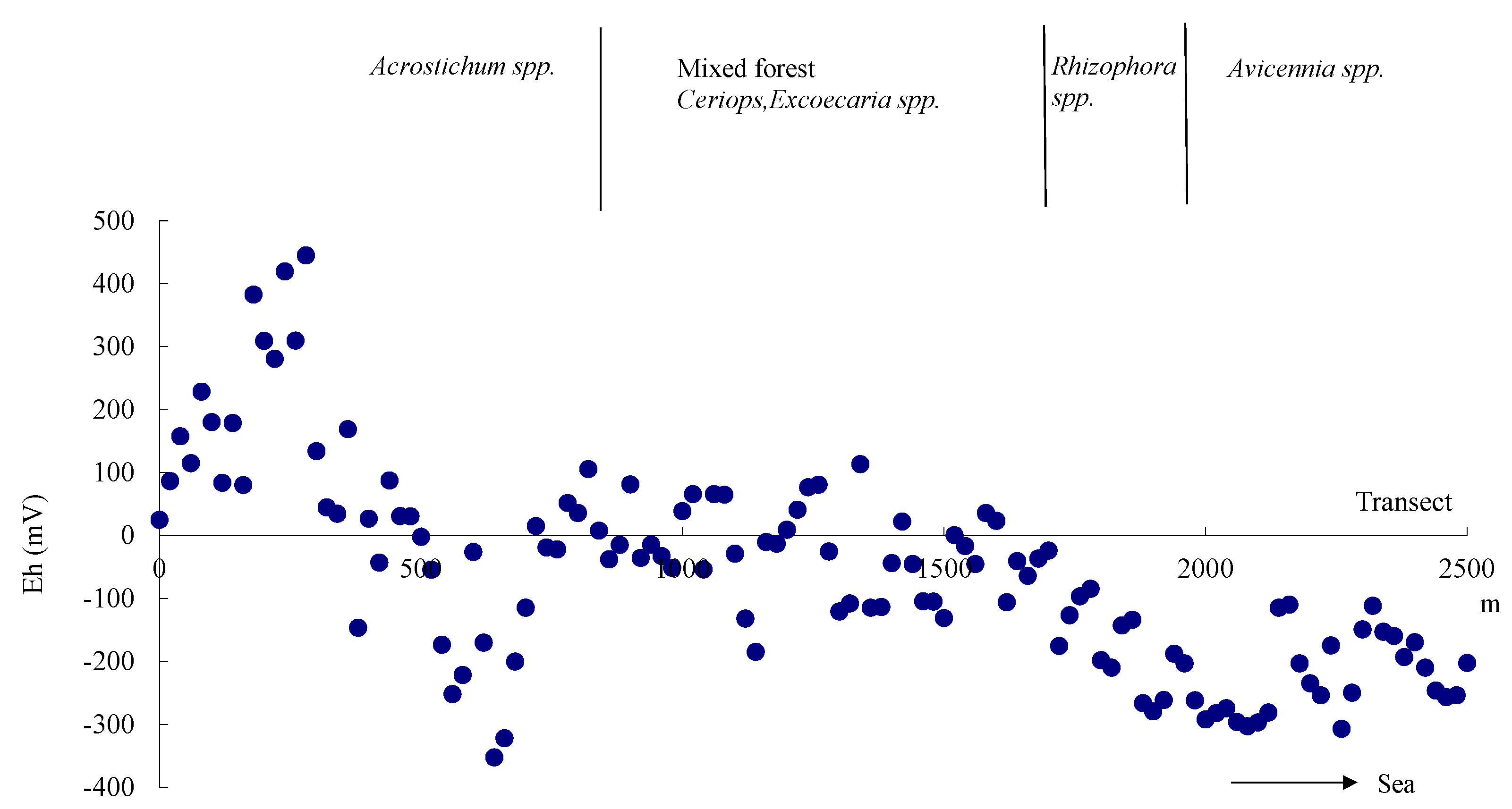
Figure 4.
Redox potential (Eh) changes along the transect. Eh decreased towards the sea.
Figure 4.
Redox potential (Eh) changes along the transect. Eh decreased towards the sea.
Eh varied markedly in the
Acrostichum spp. zone (
Figure 4). The degradation of OM, which was present at high concentrations in most wetland sediments, was partly responsible for the variation of sediment Eh [
36]. The high variability of Eh was attributable to the variable redox state brought about by undulating microtopography, which created different conditions for the degradation of OM by location.
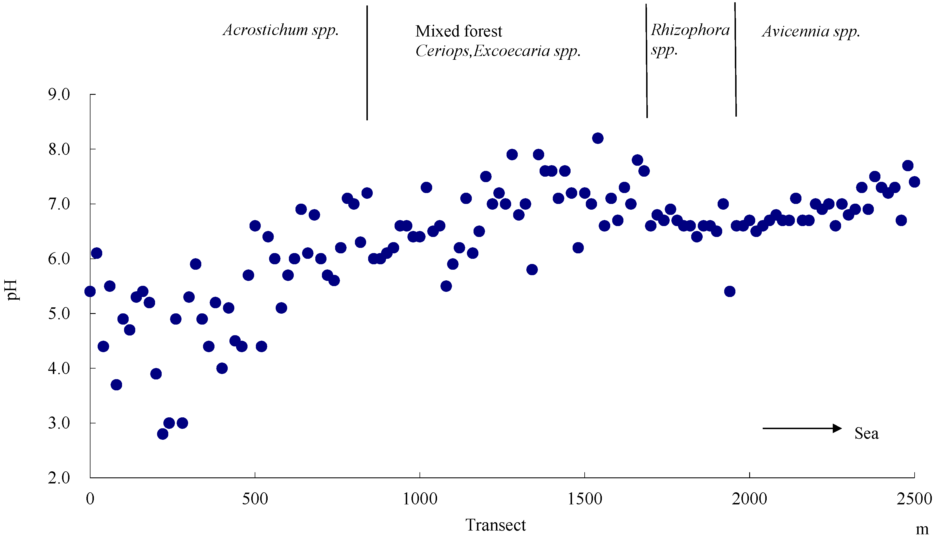
Figure 5.
pH changes along the transect. The low pH in Acrostichum spp. zone is due to rapid OM decomposition.
Figure 5.
pH changes along the transect. The low pH in Acrostichum spp. zone is due to rapid OM decomposition.
Eh was rather low in the area around 600 m from the start of the transect. The rapid oxygen consumption by aerobic microorganisms, which was driven by the high OM content, generated a strong anaerobic condition. pH in the
Acrostichum spp. zone was significantly different from that of the mangrove zone (
p < 0.01); the mean pH in the
Acrostichum spp. zone was 4.67 (
n = 19) and that of the mangrove zone was 6.08 (
n = 42). The pH values in the area at 200 m were lower than 3 as a result of the strong acidification (
Figure 5). Human disturbance in the form of excavation, which led to soil oxidation, might have caused the generation of extremely acidic soil.
Eh increased slightly in the area around 2300 m in the
Avicennia spp. zone. Nevertheless, no significant difference was found by statistical analysis. It was reported that Eh was significantly different between the
Avicennia spp. zone and the
Rhizophora spp. zone because of the difference in litter composition [
37] and in OM decomposability [
16]. As the major organic materials entering the coastal ecosystem were plant litter and root exudates, the significant differences in Eh among the areas are related to the differences in mangrove species.
3.2. OC in Surface Soils
Surface soil OC contents were higher in the mangrove areas than in the terrestrial areas (
Table 4), implying that the mangrove ecosystem had higher capacity for OM production and storage. At NR2, a sampling point in the
Acrostichum spp. zone, total carbon content was the highest at 14.2%. NR1, another sampling point in the
Acrostichum spp. zone, also had high total carbon content, as shown by the mean OC values of 17.6% in the
Acrostichum spp. zone (
n = 19) and 5.1% in the mangrove area (
n = 42) with a significance level of
p < 0.05. It was speculated that
Acrostichum spp. would have the capacity to produce a large amount of OM. Meanwhile, OC content in PF was low. As PF was originally a mangrove before the 1980s, carbon was lost by land use change. A significant amount of carbon might have been lost from the coastal ecosystem, considering that a large mangrove area was converted into shrimp ponds in the study area.
Figure 6.
OC contents and C/N ratios in surface soils collected at 5 cm soil depth along the transect. Note that soil from Acrostichum spp. zone had high OC content and C/N ratio was low near the shoreline.
Figure 6.
OC contents and C/N ratios in surface soils collected at 5 cm soil depth along the transect. Note that soil from Acrostichum spp. zone had high OC content and C/N ratio was low near the shoreline.
The C/N ratio of topsoil decreased seaward (
Figure 6), but increased from the upper layer to the lower layer (
Table 4). The C/N ratio was often used as an indicator of the source of OM in aquatic sediments. The C/N ratio in aquatic systems was governed by the mixing of terrestrial and autochthonous OM [
38,
39]. OM derived mainly from plankton had a C/N ratio of 6 to 9 [
40,
41], whereas OM derived from terrestrial vascular plants and their derivatives in sediments had a C/N ratio of 15 or higher [
42,
43]. Therefore, the low C/N ratio in
Avicennia spp. zone could be influenced by carbon originating from biological sources, such as plankton or algae.
Correlation analysis of soil properties was conducted in 74 surface soil samples collected along the transect (
Table 5). In the surface soil samples, pH was correlated to C% (
r = −0.66,
p < 0.01). Organic acids released by OM decomposition increased acidity. pH was also influenced by the reductive condition (Eh) (
r = −0.58,
p < 0.01). The strong correlation between carbon and nitrogen indicated that carbon was the major source of nitrogen. The majority of nitrogen in the soil samples existed in the organic form. After decomposition by microorganisms (mineralization), organic nitrogen was transformed into inorganic nitrogen in the form of NH
4 or NO
3, which are the available forms of nitrogen for utilization by plants. Mineralization provided much of the nitrogen needed to maintain high primary production in mangrove forests [
44,
45] and salt marshes [
46].
Table 5.
Correlation matrix of surface soil properties along the transect (n = 74).
Table 5.
Correlation matrix of surface soil properties along the transect (n = 74).
| C% | N% | CN ratio | pH | Eh |
|---|
| N% | 0.83 * | | | | |
| CN ratio | 0.34 ** | −0.09 | | | |
| pH | −0.66 * | −0.58 * | −0.13 | | |
| Eh | 0.33 ** | 0.30 ** | 0.17 | −0.58 * | |
| EC (ms/cm) | −0.37 ** | −0.29 ** | −0.20 | 0.35 ** | −0.17 |
The relatively weak correlation between carbon and C/N ratio meant that there were a number of carbon sources and different degrees of biological activity. Carbon source would primarily originate from vegetation or plankton, and its decomposability would be affected by both the chemical constituents in OM and the condition of the soil, i.e., its pH and Eh.
Figure 7.
Belowground OC and N contents, and C/N ratios at different depths along the transect. Note that the mangrove mud layer had higher OC content and lower C/N ratio than the other layers.
Figure 7.
Belowground OC and N contents, and C/N ratios at different depths along the transect. Note that the mangrove mud layer had higher OC content and lower C/N ratio than the other layers.
3.4. Leaf Analysis
Chemical element uptake was significantly greater in plants grown under wetland conditions than in those grown under dryland conditions [
47]. Compared with the terrestrial ecosystem, Na, P, Mg, and Cl showed greater accumulation in the flooded zone, including the mangrove area (
Table 6,
Figure 7). An increase of Na content in leaf was noted along the transect (
Figure 8). This tendency corresponded to the salt tolerance of mangrove species. Na content in major mangrove species was higher than 15 g/kg, markedly contrasting that of terrestrial plants, which was less than 5 g/kg (
Figure 7). The significantly high Na content in sedge, the dominant plant species in salt marsh, could be due to its selective absorption capacity. Eh and pH gradients played an important role in the mobility and uptake of P and Mg. P became available when pH became alkaline. Therefore, mangrove plants absorbed more P than terrestrial plants.
Table 6.
Macro and micro element concentrations (g/kg) determined by leaf analysis.
Table 6.
Macro and micro element concentrations (g/kg) determined by leaf analysis.
| Vegetation | Na | Mg | Al | Si | P | S | Cl | K | Ca | Mn | Fe |
|---|
| SF 1 | 1.20 | 1.29 | 0.08 | 0.82 | 0.16 | 4.63 | 12.9 | 2.54 | 9.02 | 1.01 | 0.23 |
| SF 2 | 0.15 | 8.03 | 0.05 | 0.77 | 0.23 | 7.03 | 5.4 | 3.97 | 10.53 | 1.70 | 0.22 |
| Coconut | 2.27 | 2.20 | 0.05 | 2.63 | 0.22 | 7.92 | 8.4 | 3.13 | 5.30 | 0.21 | 0.18 |
| Rice | 1.58 | 0.94 | 0.02 | 0.74 | 0.51 | 9.52 | 56.8 | 14.40 | 1.79 | 0.06 | 0.47 |
| Sedge | 29.09 | 1.18 | 0.01 | 0.22 | 0.23 | 16.44 | 125.0 | 17.21 | 2.02 | 0.03 | 0.14 |
| Acrostichum | 8.67 | 5.02 | 0.02 | 0.18 | 0.25 | 11.54 | 39.5 | 18.56 | 12.38 | 0.10 | 0.11 |
| Excoecaria | 2.60 | 3.02 | 0.04 | 0.41 | 0.32 | 11.43 | 45.7 | 9.85 | 1.70 | 0.19 | 0.25 |
| Ceriops | 8.54 | 9.79 | 0.06 | 0.06 | 0.23 | 29.14 | 54.0 | 6.29 | 14.08 | 0.23 | 0.17 |
| Bruguiera | 21.25 | 8.05 | 0.07 | 0.08 | 0.23 | 10.84 | 144.9 | 5.97 | 19.48 | 0.27 | 0.12 |
| Rhizophora | 16.38 | 7.37 | 0.34 | 0.21 | 0.38 | 4.61 | 0.0 | 8.87 | 9.54 | 0.46 | 0.36 |
| Sonneratia | 25.31 | 6.17 | 0.07 | 0.14 | 0.45 | 14.18 | 123.9 | 7.79 | 7.73 | 1.07 | 0.17 |
| Avicennia | 26.59 | 4.57 | 0.02 | 0.10 | 0.44 | 7.07 | 49.0 | 13.99 | 5.23 | 0.27 | 0.07 |
Figure 8.
Leaf Na, P, Mg, and Cl contents in different types of vegetation along the transect. SF denotes secondary forest.
Figure 8.
Leaf Na, P, Mg, and Cl contents in different types of vegetation along the transect. SF denotes secondary forest.
Significant differences were noted for particular elements among the three mangrove species. Fe content was high in Rhizophora leaf tissues, whereas Al, Mn, and S contents were high in Avicennia, Sonneratia, and Ceriops, respectively. Thus, mangrove species appeared to have uptake preference for elements, and this might indicate their possible use as ecological indicators for inorganic compound monitoring in mangrove ecosystems.
3.5. Radio Carbon Dating Analysis
The formation of the mud layer started around 6460–7030
14C years BP, as shown in the radiocarbon dating of mud layer bottom (NR2, 6462; NR3, 7540; NR4, 7030
14C years BP) (
Table 7). As Fujimoto
et al. [
48] reported, the first regression occurred before 7200
14C years BP in the southwestern coast of Thailand; the mud layer could have been formed during the transgression period.
Table 7.
Results of radiocarbon dating analysis.
Table 7.
Results of radiocarbon dating analysis.
| Site | Layer | Depth * | Type of sample | Measured 14C age (year BP) | δ13C (‰) | Conventional 14C age (year BP) |
|---|
| NR1 | Mangrove mud | 105–115 | organic sediment | 1820 ± 110 | −25.00 | 1820 ± 110 |
| NR2 | Mangrove mud | 100–104 | organic sediment | 1610 ± 70 | −25.70 | 1600 ± 70 |
| Shell-dominated | 400–404 | organic sediment | 6020 ± 80 | −25.90 | 6000 ± 80 |
| Mud | 530–540 | shell | 6070 ± 40 | −1.40 | 6460 ± 40 |
| NR3 | Mangrove mud | 105–112 | organic sediment | 1730 ± 100 | −24.40 | 1730 ± 100 |
| Shell-dominated | 385–393 | organic sediment | 6080 ± 80 | −25.90 | 6070 ± 80 |
| Mud | 535–542 | organic sediment | 7530 ± 40 | −24.20 | 7540 ± 40 |
| NR4 | Mangrove mud | 174–176 | shell | 1020 ± 40 | −5.80 | 1330 ± 40 |
| Shell-dominated | 387 | shell | 3400 ± 40 | 1.80 | 3840 ± 40 |
| Mud | 700–710 | organic sediment | 7050 ± 40 | −26.20 | 7030 ± 40 |
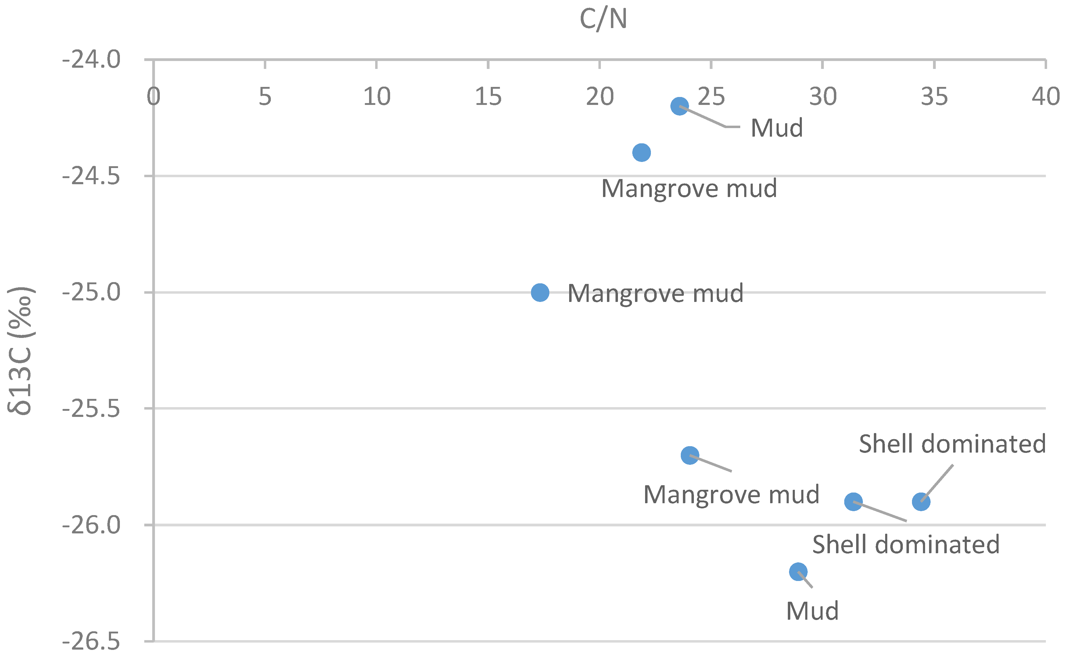
Figure 9.
δ13C values and C/N values of soils and sediments in the layers.
Figure 9.
δ13C values and C/N values of soils and sediments in the layers.
The deposition of the organic-rich mangrove mud layer started around 1330–1820
14C years BP. The sea level started to change around 2200
14C years BP in the southwestern coast of Thailand [
48]. The mangrove mud layer at the study site started to form after those periods.
A comparison of the carbon dating results obtained from different locations in the mangrove mud layer revealed that sedimentation was likely to start earlier inland than offshore. This was in agreement with the idea that the mangrove ecosystem was developing in the offshore direction. The distance between NR1 and NR4 was 2000 m, and their sedimentation times differed by 500 years. By computing those values, it was found that the mangrove would have moved 4 m seaward per year.
Bulk sediment δ13C and C/N values were the result of autochthonous inputs from wetland vegetation and allochthonous sources, such as algae and particulate organic matter [
49,
50,
51]. δ13C (‰) in organic sediment was between −26‰ and −24‰ (
Table 7), which resembled that of terrestrial carbon sources, whose range was between −33‰ and −25‰ [
52], and of fresh water phytoplankton δ13C, whose range was between −30‰ and −25‰ [
53]. However, δ13C (‰) in the mangrove mud layer varied greatly (
Figure 9), which might indicate diverse source,
i.e., not only terrestrial but also marine source.
3.6. Humic Acid Determination
The type of humic acid is representative of the deposition environment. Carboxylic humic acid is composed of aromatic compounds that are most likely derived from lignin of vascular plants [
54]. It is thought that, during humification, carboxylic acid content in OM increases [
55]. Thus, carboxylic acid content can be used as an indicator of the degree of humification.
Carboxylic acid content in the mangrove mud layer ranged from 24% to 52%, and aliphatic content, from 34% to 66% (
Table 8). Considering that carboxylic acid content and aliphatic content were generally 76%–95% and 5%–27%, respectively, in terrestrial ecosystems [
56], the mangrove OM had not yet progressively humified. Mangrove soils were mostly reductive due to waterlogging, which retarded humification.
Table 8.
Compositions (%) of humic acids at different sites and depths.
Table 8.
Compositions (%) of humic acids at different sites and depths.
| Site | Depth | Layer | Aliphatic | Phenolic | Carboxylic |
|---|
| NR1 | | Mangrove mud | 38 | 10 | 52 |
| NR2 | | Mangrove mud | 66 | 10 | 24 |
| NR3 | | Mangrove mud | 36 | 12 | 52 |
| NR4 | | | | | |
| 0–5 cm | Mangrove mud | 34 | 15 | 51 |
| 305–310 cm | Shell-dominated | 22 | 11 | 67 |
| 490–495 cm | Mud | 19 | 12 | 69 |
Humic acids at NR2 were characterized by a high aliphatic content, resembling the chemical characteristics of humic acids in sea-bottom or lake-bottom sediments. The high OC production of
A. aureum (
Figure 6) and the reductive condition (
Figure 5) might have influenced the buildup of this aliphatic-rich humic composition.
Aliphatic-rich mangrove soils are susceptible to decomposition because they are prone to oxidation [
57]. Under the aerobic condition, aliphatic compounds are easily degraded by microbial activity because the compounds possess a long aliphatic chain in their chemical structures [
56]. Land use change, such as the conversion of mangrove into shrimp pond, may cause structural changes in mangrove humic substances. Carbon decomposition will be accelerated by the decrease of moisture regime and the increase of soil temperature. Therefore, it is necessary to study the fate of mangrove OCs in relation to land use change, with water/soil condition monitoring from the viewpoint of humic substances.
Carboxylic acid content was high, and aliphatic content was low in humic acids from the shell-dominated and mud layers at NR4. The increase of the carboxylic acid content and the decrease of the aliphatic content are related to structural changes caused by the humification process. In the event of dehydration, demethylation of the aliphatic components would proceed, increasing carboxylic acid components, which are weathering-resistant components, and hence advancing humification. Sediments in the sublayers, which partly included marine-originating deposits, were mostly transported from the land. Humification of terrestrial OM took place more rapidly because the terrestrial condition was normally drier and aerobic. OM with a high degree of humification was transported from the land and deposited as sublayers; therefore, humic acids in the sublayers had high carboxylic acid content but not aliphatic content. In PF, where water was stagnant in a pond, humification did not occur progressively due to the prolonged wet condition.


