
Application of State of the Art Modeling Techniques to Predict Flooding and Waves for a Coastal Area within a Protected Bay

 ,
,
Abstract
:1. Introduction
2. Methods
2.1. Surge and Tide Water Levels
2.2. Wave Modeling
2.3. Digital Elevation Model (DEM)
3. Results and Discussion
3.1. Surge and Tide Water Levels
3.2. Wave Modeling
3.3. Simulations
4. Conclusions
4.1. Key Findings Include
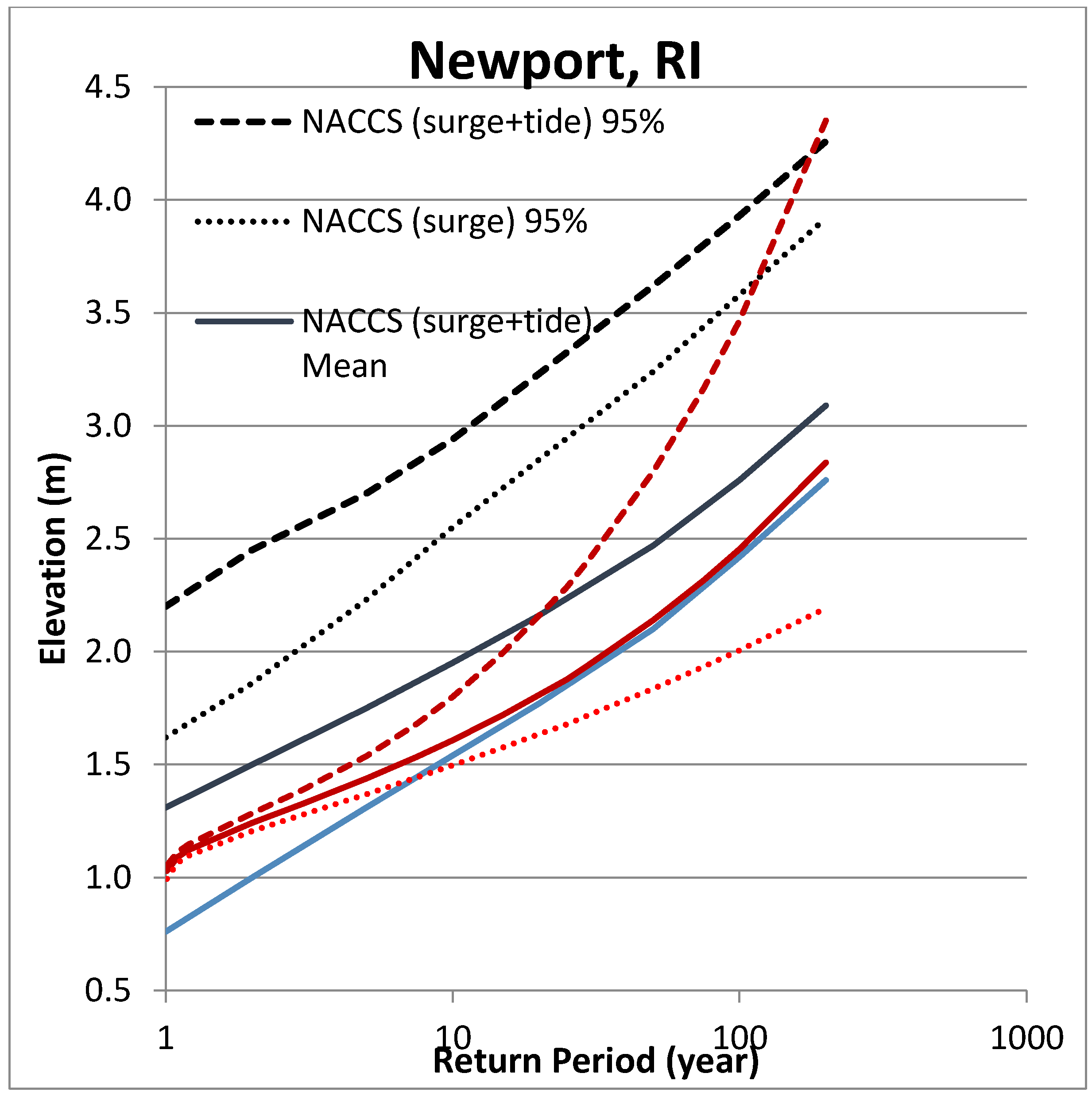
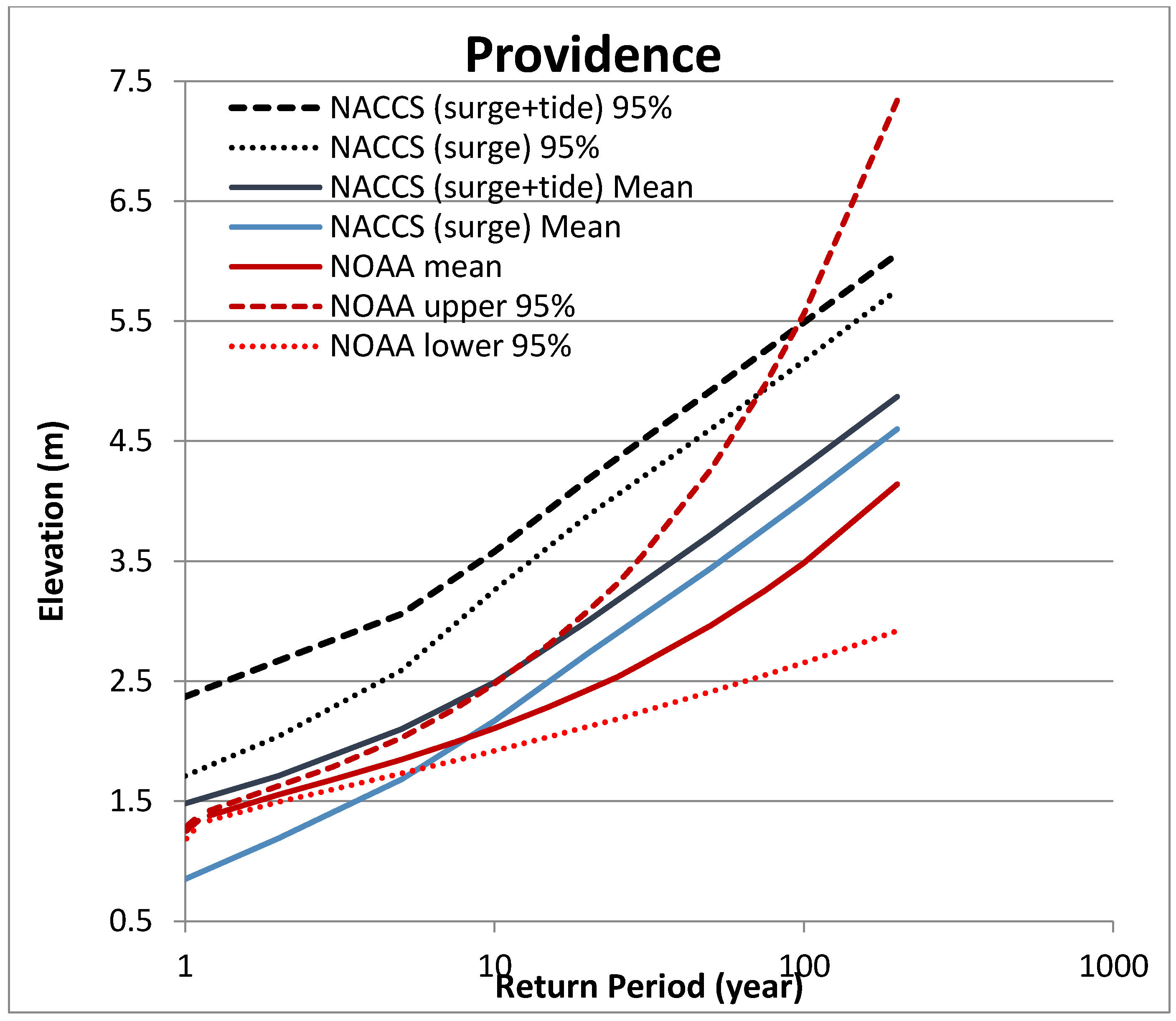
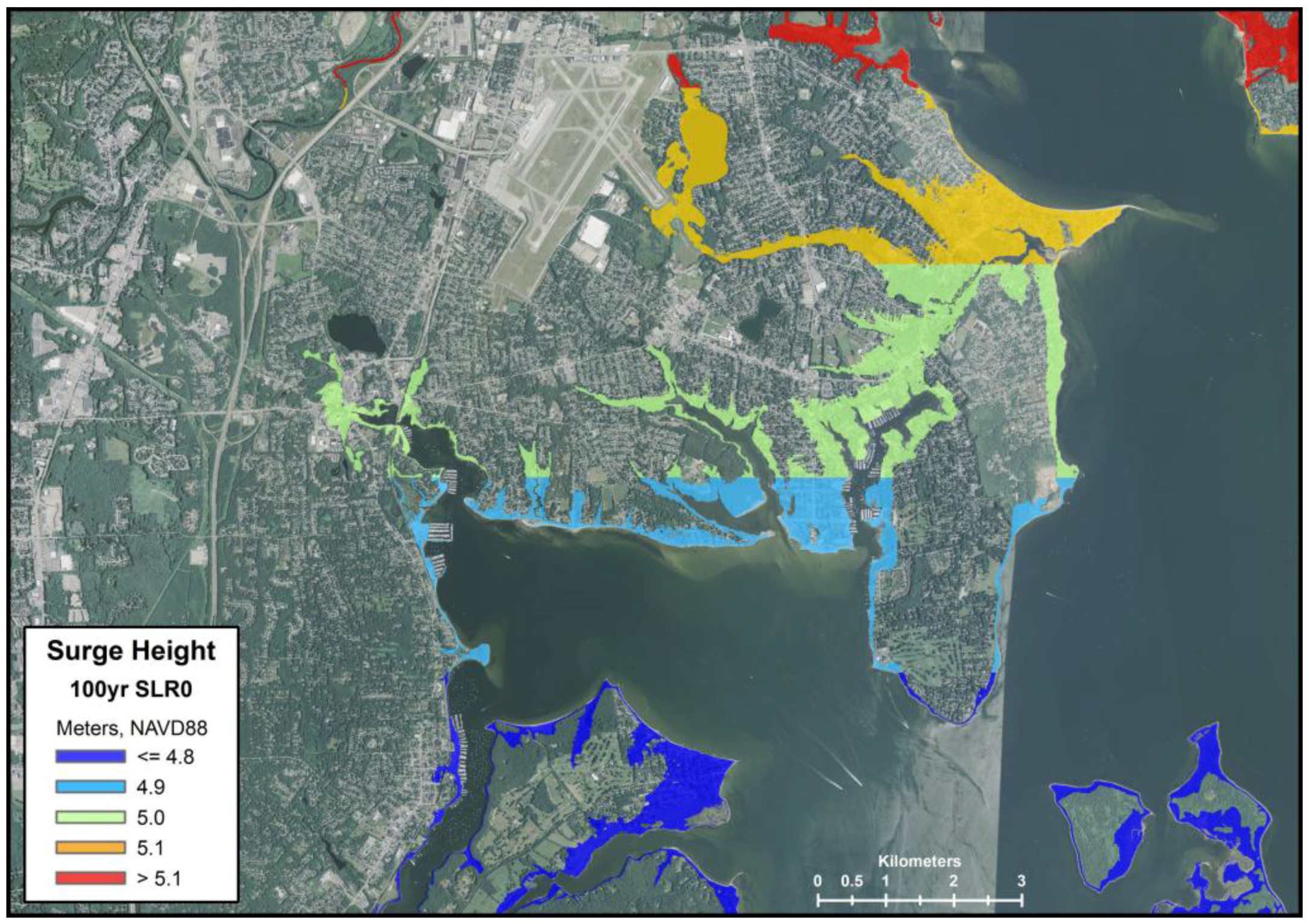
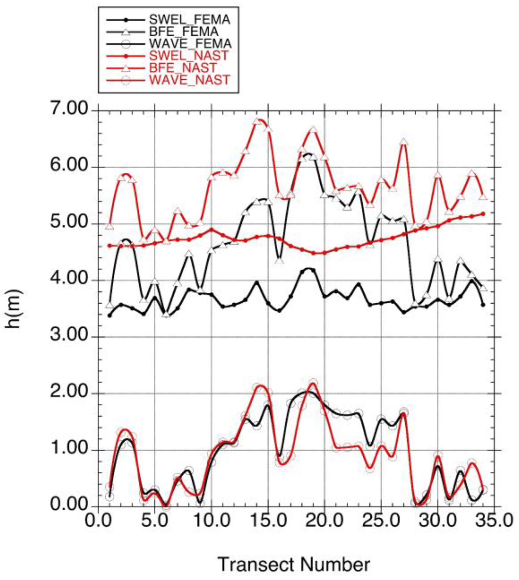
- FEMA predicted 100-year water levels (SWEL) range from 3.4 to 3.8 m for the study area. Our study results are larger (4.6 to 5.2 m); a difference of approximately 1.1 m. NAST results are approximately 30% higher than FEMA results. The larger values predicted by our analysis are attributed to the use of the upper 95% confidence limit water levels used in the present study, compared to FEMA’s return period analysis, based on the historical data. It is noted FEMA’s values are larger than the NOAA mean value, but smaller than the upper 95% for both Newport and Providence; all using the same historical data set. Hence, the difference is due to use of a different extremal value analysis method. Since NOAA has primary authority for collecting and analyzing the water level data, it is unclear why FEMA would choose an alternative method that gives predictions at variance with NOAA’s values.
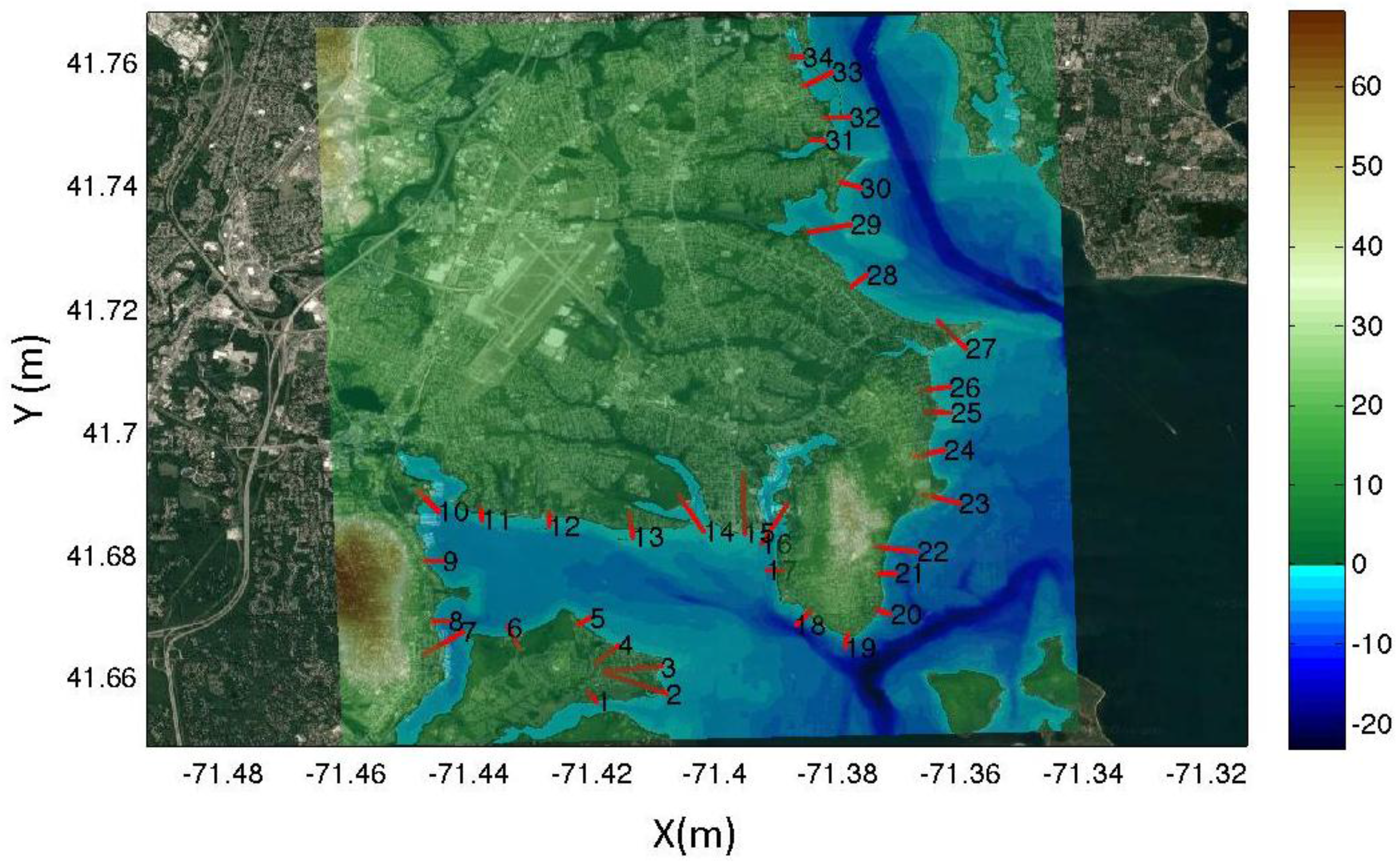
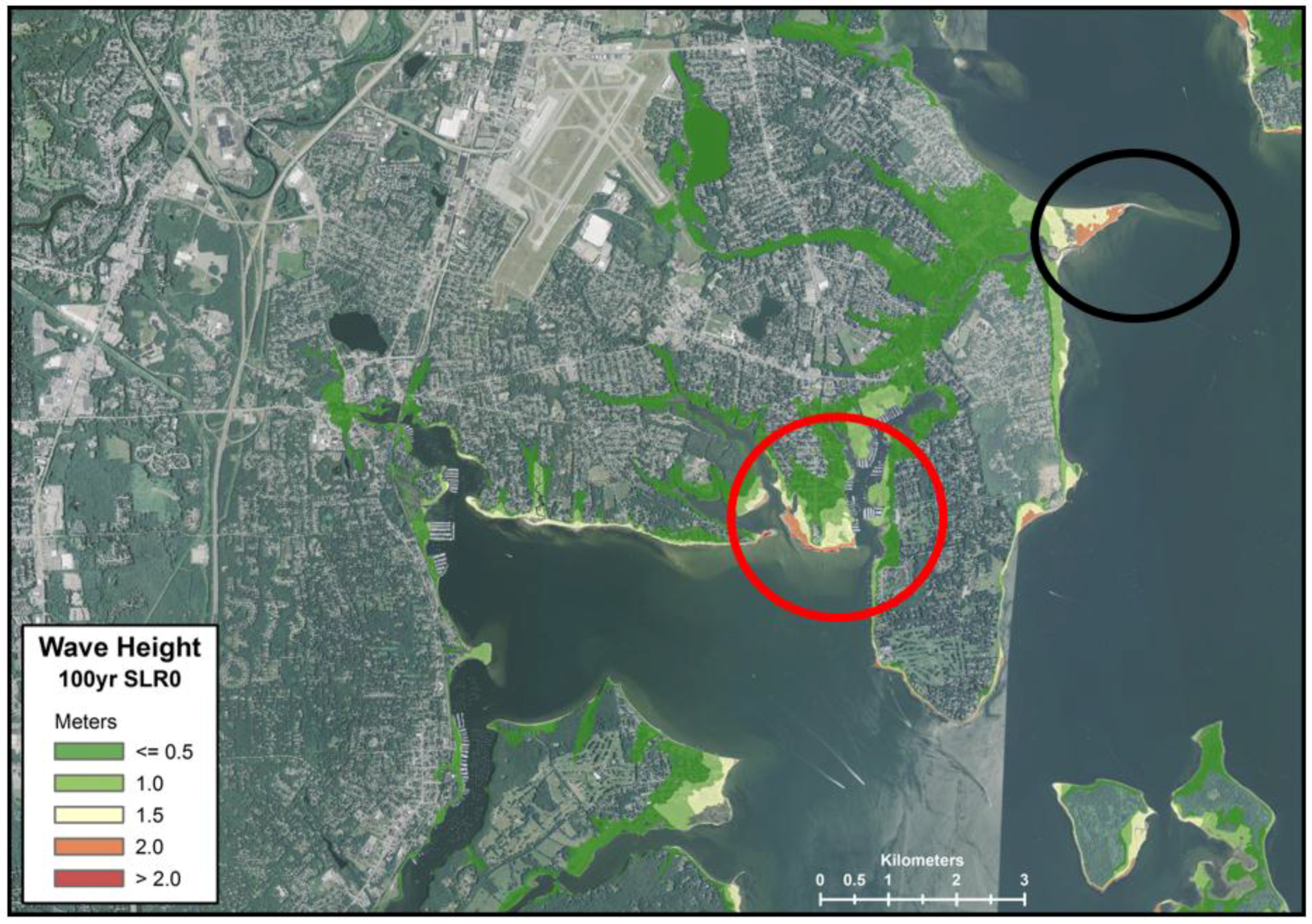
- The comparison of FEMA and NAST wave predictions show comparable results for wave heights (0.5 to 2 m), with the spatial variations controlled by the maximum fetch distance to the south. On average, across all transects, NAST model predictions are approximately 7% lower than FEMA. This small difference is explained by the fact that FEMA’s method and the current STWAVE-based approach are both dominated by fetch distances along the central axis of the West Passage of Narragansett Bay, from the south.
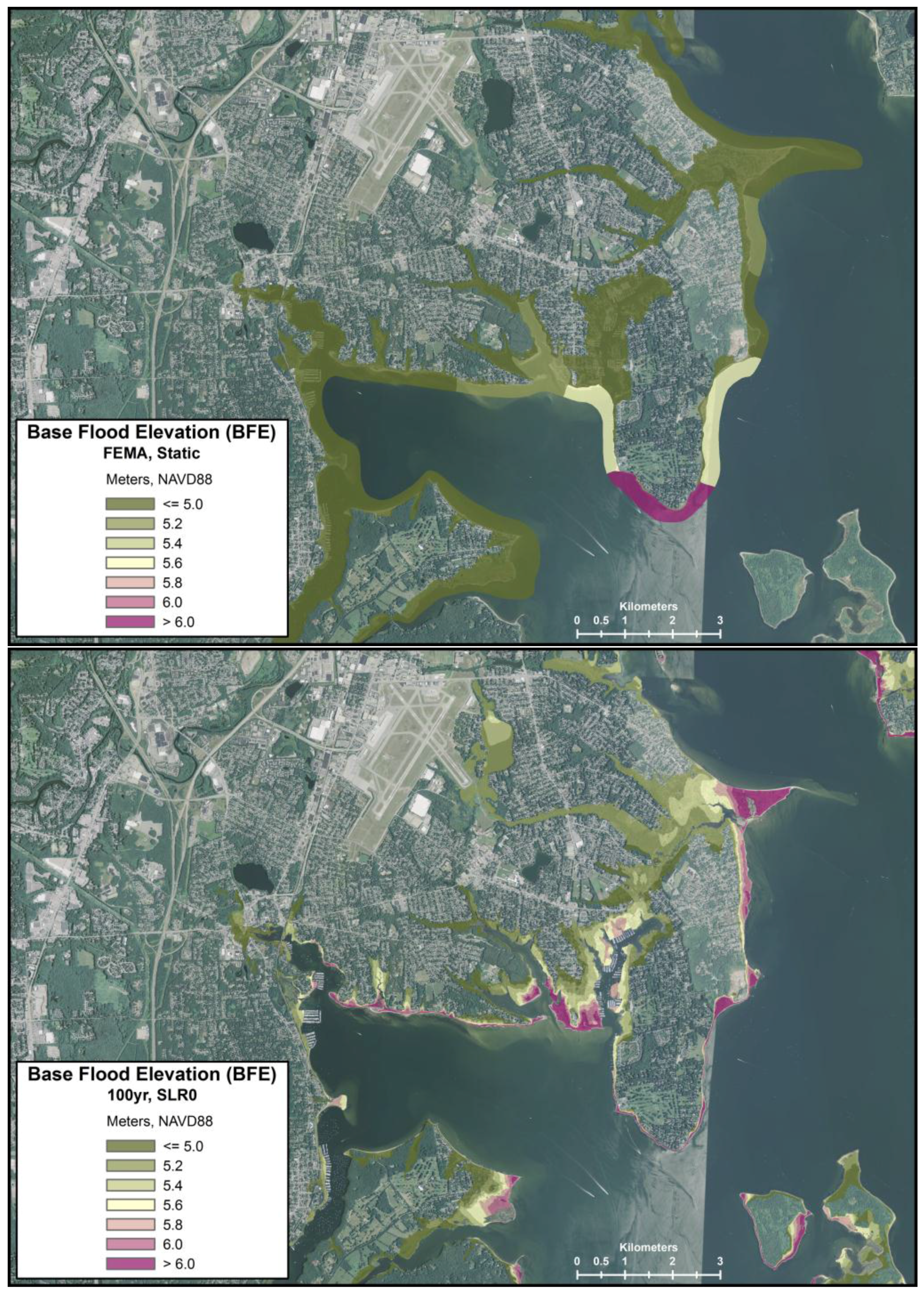
- FEMA BFE maps show strong variations between transect lines, reflecting the subjective nature of the interpolation of the 2-D maps from the 1-D transects. NAST results, on the other hand, show the importance of 2-D wave transformation processes and the spatial scales are consistent with the topography and bathymetry of the study area.
- It has proven impossible to recreate the 2-D structure of the wave field in the flood inundated area that FEMA has developed, given the results for the FIS transects. It seems to be primarily controlled by topography. The FIS transect spacing is too large to determine the spatial structure and the 2-D wave processes are not represented by the WHAFIS method used.
- The mean BFE value, averaged over all transects, is approximately 22% larger, based on the NAST analysis, compared to the FEMA results. The difference is attributed to the 30% higher SWEL for the NAST data, compared to the FEMA value and slightly lower (7%) wave crest heights.
4.2. Open Coast vs. Protected Bay Area
4.3. Some Lessons Learned
- Given the uncertainty in the various modeling and return period analysis methods employed to determine the water flood level, it seems prudent to develop a quantitative measure of the uncertainty of the results. The use of the upper 95% confidence limit value addresses both issues, is readily available, and simple to implement and understand.
- It is clear that the application of WHAFIS and the subsequent interpolation of its 1-D results to generate a 2-D map is problematic. The boundary conditions for the end of the WHAFIS transects and the assumption about the profile for the eroded dune are both issues. As noted in the NRC review and documented here, wave transformation is a 2-D process that cannot be represented in a 1-D model. WHAFIS should be replaced by a suitable 2-D model (e.g., STWAVE).
- Given the evolution of fully coupled, time dependent flood inundation and wave models on the international scale, it would be appropriate for FEMA to update the list of accepted models to include those providing a more comprehensive treatment of the underlying physics and improved predictive performance.
Acknowledgments
Author Contributions
Conflicts of Interest
Acronyms
| ADCIRC | ADvanced CIRCulation model |
| ANN | Artificial Neural Network |
| BCP | Blind Control Points |
| BFE | Base Flood Elevation |
| CERI | Coastal Environmental Risk Index CHAMP-Coastal Hazard Analysis and Modeling Program |
| CH3D | Coastal Hydrodynamic Model 3D |
| CI | Confidence Interval |
| CRMC | RI Coastal Resources Management Council |
| Deltf3D | Delft 3D hydrodynamics model |
| DEM | Digital Elevation Model |
| FEMA | Federal Emergency Management Agency |
| FIRM | Flood Insurance Rate Maps |
| FIS | Flood Insurance Study |
| FUNWAVE | Boussinesq Wave Model |
| FVCOM | Finite Volume Coastal Ocean Model |
| GEV | Generalized Extreme Value |
| HUD | Housing and Urban Development |
| LAG | Lowest Adjacent Grade |
| LIDAR | Laser Imaging, Detection, and Ranging |
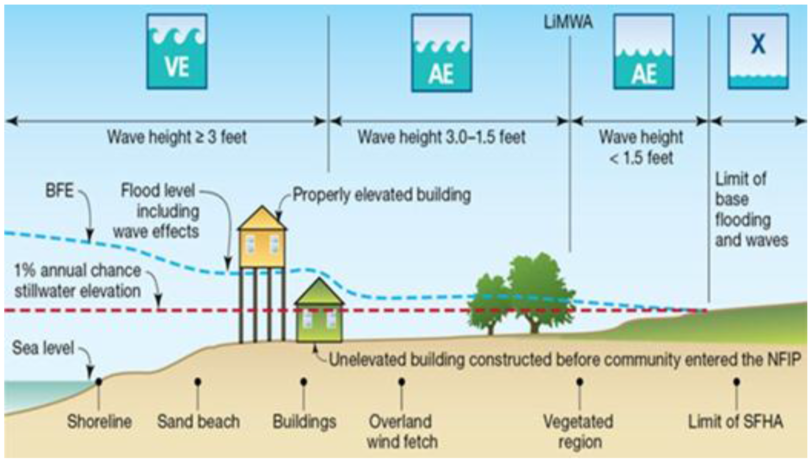
| LiMWA | Limit of Moderate Wave Action |
| MSL | Mean Sea Level |
| NACCS | USACE, North Atlantic Comprehensive Coastal Study |
| NAST | North Atlantic Coast Comprehensive Study-STWAVE |
| NAVD88 | North Atlantic Vertical Datum, 1988. |
| NOAA NOS | National Ocean and Atmospheric Administration-National Ocean Survey |
| OHCD | Office of Housing and Community Development |
| RI GIS | Rhode Island-Geographic Information System |
| RMSE | Root Mean Square Error |
| SAMP | Special Area Management Plan |
| SLR | Sea Level Rise |
| STWAVE | STeady state spectral WAVE model |
| STORMTOOLS | tools in support of storm analysis |
| SWAN | Delft 3rd generation wave model |
| SWASH | Delft Hydraulics Unsteady Flow Model |
| SWEL | Still Water Elevation |
| TELEMAC-MASCARE | suite of finite element hydrodynamic program |
| TMA | Texel, Marsen, and Arsloe wave spectrum |
| URI | University of Rhode Island |
| USACE | US Army Corp of Engineers |
| WAM | Wavewatch III, Model |
| WHAFIS | Wave Height Analysis for Flood Insurance Studies |
| WIS | USACE Wave Information Study |
| XBeach | Deltares 2D wave and sediment transport model |
Appendix A

| KENT County 100-Year Storm Water Level | |||||||||
|---|---|---|---|---|---|---|---|---|---|
| Transect Number | NAST-STORMTOOL | FEMA | Difference [NAST-FEMA] | ||||||
| SWEL (m) | BFE (m) | WAVE (m) | SWEL (m) | BFE (m) | WAVE (m) | SWEL (m) | BFE (m) | WAVE (m) | |
| 1 | 4.62 | 4.96 | 0.35 | 3.38 | 3.57 | 0.18 | 1.23 | 1.40 | 0.17 |
| 2 | 4.61 | 5.82 | 1.32 | 3.57 | 4.66 | 1.1 | 1.04 | 1.16 | 0.22 |
| 3 | 4.61 | 5.79 | 1.24 | 3.51 | 4.63 | 1.13 | 1.10 | 1.15 | 0.11 |
| 4 | 4.62 | 4.73 | 0.11 | 3.41 | 3.66 | 0.24 | 1.21 | 1.08 | −0.13 |
| 5 | 4.66 | 4.90 | 0.24 | 3.69 | 3.99 | 0.3 | 0.97 | 0.90 | −0.06 |
| 6 | 4.70 | 4.70 | 0.00 | 3.38 | 3.41 | 0.03 | 1.32 | 1.29 | −0.03 |
| 7 | 4.72 | 5.24 | 0.52 | 3.51 | 3.96 | 0.46 | 1.22 | 1.28 | 0.06 |
| 8 | 4.72 | 4.98 | 0.26 | 3.84 | 4.48 | 0.64 | 0.88 | 0.50 | −0.38 |
| 9 | 4.80 | 5.03 | 0.24 | 3.78 | 3.84 | 0.06 | 1.02 | 1.19 | 0.18 |
| 10 | 4.90 | 5.83 | 0.93 | 3.75 | 4.54 | 0.79 | 1.15 | 1.29 | 0.14 |
| 11 | 4.80 | 5.92 | 1.14 | 3.54 | 4.63 | 1.1 | 1.27 | 1.29 | 0.04 |
| 12 | 4.72 | 5.86 | 1.15 | 3.57 | 4.69 | 1.13 | 1.15 | 1.17 | 0.02 |
| 13 | 4.71 | 6.29 | 1.61 | 3.66 | 5.21 | 1.55 | 1.05 | 1.08 | 0.06 |
| 14 | 4.77 | 6.82 | 2.11 | 3.96 | 5.4 | 1.43 | 0.81 | 1.43 | 0.68 |
| 15 | 4.79 | 6.69 | 2.02 | 3.6 | 5.4 | 1.8 | 1.19 | 1.29 | 0.22 |
| 16 | 4.74 | 5.51 | 0.78 | 3.47 | 4.36 | 0.88 | 1.26 | 1.15 | −0.10 |
| 17 | 4.61 | 5.51 | 0.90 | 3.72 | 5.55 | 1.83 | 0.89 | −0.04 | −0.93 |
| 18 | 4.55 | 6.33 | 1.79 | 4.15 | 6.16 | 2.01 | 0.40 | 0.18 | −0.22 |
| 19 | 4.49 | 6.68 | 2.19 | 4.18 | 6.19 | 2.01 | 0.31 | 0.49 | 0.18 |
| 20 | 4.49 | 6.19 | 1.70 | 3.72 | 5.52 | 1.8 | 0.77 | 0.67 | −0.10 |
| 21 | 4.55 | 5.59 | 1.04 | 3.81 | 5.46 | 1.65 | 0.74 | 0.13 | −0.60 |
| 22 | 4.60 | 5.64 | 1.05 | 3.69 | 5.3 | 1.62 | 0.91 | 0.34 | −0.56 |
| 23 | 4.60 | 5.67 | 1.07 | 3.93 | 5.58 | 1.65 | 0.67 | 0.10 | −0.57 |
| 24 | 4.67 | 5.35 | 0.68 | 3.57 | 4.63 | 1.07 | 1.10 | 0.71 | −0.39 |
| 25 | 4.72 | 5.79 | 1.08 | 3.6 | 5.15 | 1.55 | 1.12 | 0.63 | −0.48 |
| 26 | 4.75 | 5.63 | 0.88 | 3.63 | 5.06 | 1.43 | 1.13 | 0.57 | −0.55 |
| 27 | 4.82 | 6.46 | 1.68 | 3.44 | 5.09 | 1.65 | 1.37 | 1.37 | 0.03 |
| 28 | 4.88 | 4.98 | 0.09 | 3.54 | 3.6 | 0.06 | 1.35 | 1.38 | 0.03 |
| 29 | 4.93 | 5.05 | 0.12 | 3.54 | 3.75 | 0.21 | 1.39 | 1.30 | −0.09 |
| 30 | 4.96 | 5.87 | 0.91 | 3.66 | 4.39 | 0.73 | 1.31 | 1.48 | 0.18 |
| 31 | 5.06 | 5.23 | 0.16 | 3.57 | 3.69 | 0.12 | 1.50 | 1.54 | 0.04 |
| 32 | 5.11 | 5.49 | 0.38 | 3.72 | 4.36 | 0.64 | 1.40 | 1.13 | −0.26 |
| 33 | 5.13 | 5.90 | 0.78 | 3.99 | 4.11 | 0.12 | 1.14 | 1.79 | 0.65 |
| 34 | 5.18 | 5.48 | 0.30 | 3.57 | 3.87 | 0.3 | 1.61 | 1.61 | 0.00 |
| Mean | 4.75 | 5.64 | 0.91 | 3.67 | 4.64 | 0.98 | 1.08 | 1.0 | −0.07 |
| Minimum | 0.31 | −0.04 | −0.93 | ||||||
| Maximum | 1.61 | 1.79 | 0.68 | ||||||
| Standard Deviation | 0.28 | 0.48 | 0.34 | ||||||
| RMS | 1.12 | 1.11 | 0.34 | ||||||
References
- Federal Emergency Management Agency (FEMA). Atlantic Ocean and Gulf of Mexico Coastal Guidelines Update; FEMA: Washington, DC, USA, 2007.
- Federal Emergency Management Agency. Flood Insurance Study, Kent County, RI, FEMA Flood Insurance Study Number 44003CV000B; FEMA: Washington, DC, USA, 2012.
- Federal Emergency Management Agency. Updated Tidal Profiles for the New England Coastline. March 2012. Available online: https://www.fema.gov/media-library/assets/documents/85240 (accessed on 16 January 2017). [Google Scholar]
- Federal Emergency Management Agency. WHAFIS Documentation Version 4.0. 2007. Available online: https://www.fema.gov/wave-height-analysis-flood-insurance-studies-version-40 (accessed on 16 January 2017). [Google Scholar]
- National Research Council. Mapping the Zone: Improving Flood Map Accuracy; Committee on FEMA Flood Maps; Board on Earth Sciences and Resources/Mapping Science Committee; National Research Council: Washington, DC, USA, 2009. [Google Scholar]
- FEMA Definitions. Available online: https://www.fema.gov/sites/default/files/images/flood_zones_limwa.jpg (accessed on 16 January 2017).
- Spaulding, M.L.; Grilli, A.; Damon, C.; Oakley, B.; Fugate, G.; Isaji, T.; Schambach, L. Application of state of art modeling techniques to predict flooding and waves for an exposed coastal area. J. Mar. Sci. Eng. 2017, 5, 10. [Google Scholar] [CrossRef]
- FEMA Approved Models. Available online: https://www.fema.gov/coastal-numerical-models-meeting-minimum-requirement-national-flood-insurance-program (accessed on 17 January 2017).
- Cialone, M.A.; Massey, T.C.; Anderson, M.E.; Grzegorzewski, A.S.; Jensen, R.E.; Cialone, A.; Mark, D.J.; Pevey, K.C.; Gunkel, B.L.; McAlpin, T.O. North Atlantic Coast Comprehensive Study (NACCS) Coastal Storm Model Simulations: Waves and Water Levels; Report: ERDC/CHL TR-15-44; Coastal and Hydraulics Laboratory U.S. Army Engineer Research and Development Center: Vicksburg, MS, USA, 2015. [Google Scholar]
- Spaulding, M.L.; Isaji, T.; Damon, C.; Fugate, G. Application of STORMTOOLS’s simplified flood inundation model, with and without sea level rise, to RI coastal waters. In Proceedings of the ASCE Solutions to Coastal Disasters Conference, Boston, MA, USA, 9–11 September 2015.
- STORMTOOLS Website. Available online: http://www.beachsamp.org/resources/stormtools/ (accessed on 16 January 2017).
- Massey, T.C.; Anderson, E.M.; McKee-Smith, J.; Gomez, J.; Rusty, J. STWAVE: Steady State Spectral Wave Model. User’s Manual for STWAVE, Version 6.0; US Army Corp of Engineers, Environmental Research and Development Center: Vicksburg, MS, USA, 2011. [Google Scholar]
- Smith, J.M.; Sherlock, A.R.; Resio, D.T. STWAVE: Steady-State Wave Model User’s Manual for STWAVE, Version 3.0; ERDC/CHL SR-01–01; U.S. Army Engineering Research and Development Center: Vicksburg, MS, USA, 2001. [Google Scholar]
- Borgman, L.E.; Panicker, N.N. Design Study for a Suggested Wave Gage Array off Point Mugu, California; Technical Report Hel 1-14; Hydraulic Engineering Laboratory University of California at Berkeley: Berkeley, CA, USA, 1970. [Google Scholar]
- USACE Wave Information Study. Available online: http://wis.usace.army.mil/hindcasts.shtml?dmn=atlWIS (accessed on 17 January 2017).
- RI-GIS Digital Elevation Model. Available online: http://www.rigis.org/data/topo/2011 (accessed on 16 January 2017).
- Arcement, G.J.; Schneider, V.R. Guide for Selecting Manning’s Roughness Coefficients for Natural Channels and Flood Plains; U.S. Geological SurveyWater-Supply Paper 2339; U.S. Geological Survey: Denver, CO, USA, 1989.
- Wamsley, T.V.; Cialone, M.A.; Smith, J.M.; Ebersole, B.A.; Grzegorzewski, A.S. Influence of landscape restoration and degradation on storm surge and waves in southern Louisiana. Nat. Hazards 2009, 51, 207–224. [Google Scholar] [CrossRef]
- Zervas, C. Extreme Water Levels of the United States, 1893–2010; NOAA Technical Report NOS CO-OPS 067; NOAA: Silver Spring, MD, USA, 2013.
- Hashemi, R.; Spaulding, M.L.; Shaw, A.; Farhadi, H.; Lewis, M. An efficient artificial intelligence model for prediction of tropical storm surge. J. Nat. Hazards 2016. [Google Scholar] [CrossRef]
- Schambach, L.; Grilli, A.R.; Spaulding, M.L. Predicting the 100-year storm inundation along the Narragansett Bay shoreline. Nat. Hazard 2017. in preparation. [Google Scholar]


| Station | Water Levels (m) | ||||||
|---|---|---|---|---|---|---|---|
| NACCS | NACCS | NOAA | FEMA | ||||
| Surge + Tide | Surge | ||||||
| Mean | Upper 95% | Mean | Upper 95% | Mean | Upper 95% | FIS | |
| Providence | 4.29 | 5.49 | 4.01 | 5.17 | 3.48 | 5.56 | 4.2 |
| Newport | 2.76 | 3.93 | 2.42 | 3.58 | 2.47 | 3.47 | 3.21 |
| Scaling Relative to Newport | |||||||
| Providence | 1.55 | 1.4 | 1.66 | 1.44 | 1.41 | 1.6 | 1.31 |
| Newport | 1 | 1 | 1 | 1 | 1 | 1 | 1 |
© 2017 by the authors. Licensee MDPI, Basel, Switzerland. This article is an open access article distributed under the terms and conditions of the Creative Commons Attribution (CC BY) license ( http://creativecommons.org/licenses/by/4.0/).
Share and Cite
Spaulding, M.L.; Grilli, A.; Damon, C.; Fugate, G.; Isaji, T.; Schambach, L. Application of State of the Art Modeling Techniques to Predict Flooding and Waves for a Coastal Area within a Protected Bay. J. Mar. Sci. Eng. 2017, 5, 14. https://doi.org/10.3390/jmse5010014
Spaulding ML, Grilli A, Damon C, Fugate G, Isaji T, Schambach L. Application of State of the Art Modeling Techniques to Predict Flooding and Waves for a Coastal Area within a Protected Bay. Journal of Marine Science and Engineering. 2017; 5(1):14. https://doi.org/10.3390/jmse5010014
Chicago/Turabian StyleSpaulding, Malcolm L., Annette Grilli, Chris Damon, Grover Fugate, Tatsu Isaji, and Lauren Schambach. 2017. "Application of State of the Art Modeling Techniques to Predict Flooding and Waves for a Coastal Area within a Protected Bay" Journal of Marine Science and Engineering 5, no. 1: 14. https://doi.org/10.3390/jmse5010014
APA StyleSpaulding, M. L., Grilli, A., Damon, C., Fugate, G., Isaji, T., & Schambach, L. (2017). Application of State of the Art Modeling Techniques to Predict Flooding and Waves for a Coastal Area within a Protected Bay. Journal of Marine Science and Engineering, 5(1), 14. https://doi.org/10.3390/jmse5010014