Abstract
A computational methodology for the hydrodynamic analysis of horizontal axis marine current turbines is presented. The approach is based on a boundary integral equation method for inviscid flows originally developed for marine propellers and adapted here to describe the flow features that characterize hydrokinetic turbines. For this purpose, semi-analytical trailing wake and viscous flow correction models are introduced. A validation study is performed by comparing hydrodynamic performance predictions with two experimental test cases and with results from other numerical models in the literature. The capability of the proposed methodology to correctly describe turbine thrust and power over a wide range of operating conditions is discussed. Viscosity effects associated to blade flow separation and stall are taken into account and predicted thrust and power are comparable with results of blade element methods that are largely used in the design of marine current turbines. The accuracy of numerical predictions tends to reduce in cases where turbine blades operate in off-design conditions.
1. Introduction
Marine or hydrokinetic turbines for the production of renewable energy from tidal and ocean currents is a rapidly growing technology. Large scale installations mainly consist of horizontal axis turbines installed on structures fixed to the seabed or supported by floating platforms.
The relatively fast maturation of hydrokinetic turbine technology as compared to other ocean energy harvesting systems is partly due to experience gained over the last decades in the wind energy sector. In most cases the shape of marine turbine blades resembles wind rotor blades except for the aspect ratio that is substantially smaller to resist hydrodynamic loads in water. It is thus not surprising that Blade Element Momentum methods (simply, BEM) originally developed for wind turbines are extensively used for analysis and design of tidal and ocean current turbines, see e.g., [1]. BEM provides fast and reliable estimates of turbine performance if suitable tuning is applied to overcome important methodology weaknesses [2,3]. Specifically, blade loading is derived by prescribed lift and drag properties of two-dimensional profiles and semi-empirical three-dimensional flow corrections are necessary to account for blade tip effects, blade/hub interaction, number of blades.
In contrast to this, the hydrodynamic design of marine propellers is typically based on boundary element or panel methods that, under inviscid-flow assumptions, provide a consistent representation of the three-dimensional flow around rotors in steady or unsteady flow. To avoid confusion with blade element (momentum) methods, the terminology Boundary Integral Equation Method (BIEM) is used here. In spite of that, only few examples of applications of BIEMs to hydrokinetic turbines exist, see e.g., Young et al. [4], He et al. [5]. Results in the literature highlight the difficulty of boundary element methods to correctly describe the hydrodynamic performance of turbines designed to extract energy from an onset flow. A major difficulty is that turbine blades frequently operate at high angle of attack and viscosity induced separation and stall significantly affect generated thrust and power. Baltazar and Falcão de Campos [6,7] address the problem by proposing models to correct inviscid-flow predictions by a BIEM for three-dimensional steady flows. The lift force contribution evaluated at each blade section by BIEM is corrected by comparing viscous and inviscid flow lift coefficients of two-dimensional profiles representatives of blade sections, while blade section drag is taken from two-dimensional polar curves. The Kutta-Joukowski law is used to determine the incoming velocity to blade sections, and the viscous flow code X-Foil is used to determine polar curves. The methodology includes an iterative wake alignment model to adjust wake pitch to the local flow, while radial expansion is not modelled.
The problem is tackled in the present work by revisiting the approach in [6] and developing original viscous flow and trailing wake models that are integrated into a BIEM originally developed for marine propellers, see e.g., Salvatore et al. [8,9] and Pereira et al. [10]. In the proposed methodology, the trailing wake geometry is determined by a semi-analytical model with wake pitch alignment consistent with turbine-induced velocity perturbation calculated by BIEM and an experimental-based definition of the expansion rate of the streamtube downstream of the rotor plane. Next, a viscous flow correction is determined by comparing distributions of blade loads by BIEM and lift and drag properties of representative blade sections under viscous flow conditions obtained from available experimental data or from numerical predictions by two-dimensional viscous flow solvers. Turbine wake-induced velocity by BIEM is used to determine the effective inflow to blade sections.
The resulting methodology with Viscous-Flow Correction (VFC) is referred to here as BIEM-VFC. A validation study for the proposed computational model is addressed by considering two case studies taken from the literature with experimental results for three-bladed model turbines. Specifically, Gaurier et al. [11] present results from the first round-robin test on tidal turbines carried out in the framework of the EU-FP7 MaRINET Project [12], with turbine performance measurements from two towing tanks (Strathclyde University and CNR-INSEAN) and two flume tanks (IFREMER and CNR-INSEAN). Next, Bahaj et al. [13] present a detailed characterization of marine current turbine performance by considering the effects of blade pitch variations. For this case study, BIEM-VFC is also compared with other numerical models based on BEM and BIEM. Results of the comparative analyis provide a clear overview of the accuracy of the proposed BIEM-VFC methodology and its range of applicability as a marine current turbine analysis and design tool.
The paper is organised as follows. The theoretical and computational BIEM-VFC methodology is outlined in Section 2, with details of viscous flow and trailing wake models. The validation study is addressed in Section 3, Section 4 and Section 5, while strenghts and weaknesses of the methodology are discussed in Section 6.
2. Theoretical Model
The computational model proposed here for the hydrodynamic analysis of marine current turbines is based on a Boundary Integral Equation Method (BIEM) that is valid under inviscid flow assumptions. The methodology has been originally developed at CNR-INSEAN to study marine propulsors, see e.g., Salvatore et al. [8,9], and Pereira et al. [10].
The extension of the methodology to analyse marine turbine flows requires the introduction of suitable models to describe trailing vorticity dynamics and to correct blade loads when turbine blades undergo flow separation and stall. In this section, the original BIEM is briefly reviewed and models specifically developed for turbine trailing vorticity and viscosity effects are described in detail.
Assuming the onset flow is incompressible and inviscid, the perturbation velocity induced by the turbine may be described by a scalar potential as , and general mass and momentum equations are dramatically simplified. Mass conservation yields the Laplace equation for the perturbation velocity potential, , while the momentum equation reduces to the Bernoulli equation for pressure p
where is the free-stream reference pressure, is the inflow velocity as seen from an observer fixed with blades rotating at angular velocity while is the onset flow velocity. In case of uniform inflow aligned to turbine axis x, one has with unit vector along x, see Figure 1. Finally, is the hydrostatic head term referred to a reference vertical position .
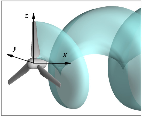
Figure 1.
Sketch of the frame of reference associated to the solid boundary describing an isolated turbine and the surface of trailing wake shed by one blade.
The Laplace equation for is solved via a boundary integral formulation where problem unknowns are distributed on the body surface and on the trailing wake surface . According to potential flow theory for lifting bodies, the trailing wake denotes a zero-thickness layer where vorticity generated by lifting surfaces is shed into the downstream flow. Through a classical derivation (see, e.g., Morino [14]) the following boundary integral representation for at an arbitrary field point is obtained
Dealing with isolated turbines modelling by BIEM, a typical schematization is to represent the device as an assembly of blades attached to a nacelle of finite length immersed in an unbounded flow, as sketched in Figure 1. As a consequence, denotes the solid surface combining blades and nacelle. Vector is the unit normal to body and wake surfaces, pointing outward on solid boundaries and from pressure to suction sides at blade trailing edges to define the orientation on the wake. The symbol in Equation (2) is used to denote discontinuity of velocity potential across the trailing wake surface defined according to the convention used for the unit normal to , whereas is a function that makes the same equation to be valid for points on the body surface () or inside the fluid domain, . Moreover, quantities are unit source and dipoles in the unbounded three-dimensional space and depend only from the mutual position between the collocation point and the influencing point on the boundary surfaces. A distinguishing feature of the present formulation is that analytical expressions are used to evaluate the exact contributions of source and dipole terms on hyperboloidal quadrilateral surface elements, see [14] for details.
Boundary conditions for the velocity potential are imposed at infinity (vanishing perturbation ), on solid surfaces (impermeability, ) and on the trailing wake, where convection of vorticity generated on blades is imposed and a Kutta-Morino condition is used to impose identity between velocity potential difference at blade trailing edge pressure and suction sides and on the wake.
Equation (2) with and related boundary conditions represents a boundary integral equation whose solution determines on the body surface. By discretizing boundaries and into surface panels, and enforcing Equation (2) at centroids of body panels, a linear set of algebraic equations is obtained. The wake surface can be determined as a part of the solution by a wake-alignment iterative procedure, as described in [15]. A faster and more robust approach is used in the present study as described in Section 2.1 below.
Once Equation (2) is numerically solved, the velocity potential and its gradient are known on the body surface and pressure can be evaluated using the Bernoulli Equation (1). Hydrodynamic loads generated by the turbine are then obtained by integrating pressure and tangential stress over the blades surface. In particular, the force contribution of a blade element of radial extension and chord c can be written as
where , is the unit vector tangent to the surface and aligned to the local flow and quantities denote, respectively, contributions by normal (pressure) and tangential (friction) stress. Integrating elementary forces on all blades, turbine thrust T and torque Q follow
Surface stress is not part of the inviscid-flow solution and could be evaluated by a coupled viscous/inviscid model in which BIEM is combined with a boundary-layer model, as described in Salvatore et al. [8]. A simplified approach popular in marine propeller models consists of estimating quantity from formulas valid for attached laminar and turbulent flow over a flat plate, see e.g., [16]
where is the friction coefficient, and
defines the Reynolds number characterizing the flow around the blade section at radius r, where is the water kinematic viscosity.
The accuracy of this approximated viscosity correction to hydrodynamic loads by BIEM is typically limited to attached flows on blade sections at low angle of attack. The VFC approach proposed here aims at coping with a wider range of conditions including flow separation and stall, as outlined in Section 2.2.
2.1. Trailing Wake Model
In the present study, a semi-analytical model is used to determine the wake surface in Equation (2). The wake is defined as a generalised helicoidal surface with distributions of axial pitch and radial expansion of the streamtube downstream of the rotor that are consistent with the operating mode of hydrokinetic turbines.
For the axial pitch, two regions are considered: the tip-vortex region and the blade wake extending spanwise between vortices released at blade root and tip. In the blade wake, trailing vortices are convected downstream with velocity given as the average of the onset flow speed and of the velocity perturbation induced by the wake itself, . A boundary integral representation of is obtained by taking the gradient of the velocity potential Equation (2). Here, an approximated representation of this velocity field across the fluid region of interest is obtained by using BIEM to evaluate at the rotor plane and imposing a linear variation downstream to match a given farfield distribution.
Then, the axial component of the wake-induced velocity, , may be written as
where is a normalised abscissa with at rotor trailing edge and at the downstream end of the discretised wake surface. Consistent with Betz theory [17], the axial induced velocity in the farfield is twice the intensity at the rotor plane. Symbol denotes the wake-induced velocity potential obtained from the gradient of the wake contribution in Equation (2), while subscript refers to the rotor plane axial position.
In the tip-vortex region, Okulov and Sørensen [18] describe a trailing vortex shedding model with axial velocity given as the average between velocity in the blade wake, Equation (7), and the unperturbed axial velocity V outside the streamtube. Thus, denoting by the hydrodynamic pitch associated to the unperturbed flow, one obtains the following expressions for the wake pitch
where pedices and denote, respectively, blade wake and tip vortex, and is a radial weight function (in the present analysis, has been used, where R is the turbine radius). In the evaluation of , the blade wake pitch is evaluated at a representative radial station .
Next, the radial expansion of the wake streamtube downstream of the rotor plane is determined as
where constants are derived from experimental data describing the wake evolution of hydrokinetic turbines over a range of operating conditions. In the present study, two datasets are considered: Micek et al. [19] with wake flow measurements up to 10 diameters downstream of a three-bladed turbine with 3% onset flow turbulence, and Del Frate et al. [20] fitting measurements in the axial range and the limit at infinite distance downstream of the rotor from Betz theory, . Results extracted from the two datasets and the analytical expansion law from Equation (9) with are illustrated in Figure 2. It should be noted that at large axial distance from the rotor, the proposed law determines an expansion rate that is intermediate between idealised conditions from the Betz theory and real conditions affected by non negligible background turbulence.
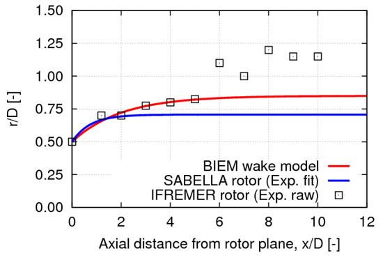
Figure 2.
Streamtube radius downstream of rotor plane from Equation (9) and comparative data from experiments.
Combining Equations (7) to (9), the generalised helicoidal surface defining the trailing wake is obtained. In fact, the evaluation of the velocity potential in Equation (7) depends on the definition of surface in Equation (2) and hence an iterative procedure is required. In the numerical analysis addressed in the present work, it has been found that the iteration converges after few steps.
2.2. Viscous-Flow Correction Model
Assumptions of inviscid, irrotational flow underlying BIEM yield that turbine hydrodynamics is studied by fast numerical solutions of a linear problem with unknowns distributed only on the solid surface of the turbine. Unfortunately, turbine performance is dramatically affected by blade flow separation and stall and hence neglecting viscosity effects may result into completely unreliable predictions of turbine hydrodynamic loads and power output.
A methodology is proposed here to correct blade loads predicted under inviscid-flow assumptions by a procedure that preserves the reduced computing effort typical of BIEM. The idea is to (i) identify conditions where blade flow is subject to boundary layer separation and stall and (ii) estimate the effect of viscosity on blade loads under such conditions. The BIEM model including this viscous flow correction is hereafter referred to as BIEM-VFC.
For this purpose, sectional loads along blade span evaluated by BIEM are compared to lift and drag properties of two-dimensional (2D) profiles describing blade sections. Equivalence between operating conditions of three-dimensional rotating blade sections and corresponding 2D profiles is enforced in terms of local Reynolds number (see Section above) and of the effective angle of attack .
Quantity defines the angle of attack where wake-induced velocity contributions are accounted for to evaluate the total velocity incoming to blade sections. A graphical definition of is given in Figure 3, where inflow velocity components and hydrodynamic force components for a turbine blade section at radius r are sketched. Axial and tangential induced velocity components, respectively and , represent three-dimensional flow effects induced by trailing vortices shed by blades. These quantitites are zero in case of 2D flow around a lifting surface of infinite span and the effective and nominal angle of attack coincide.
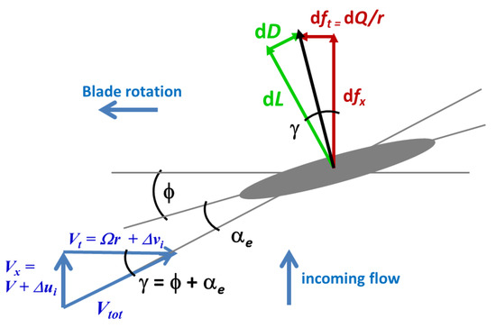
Figure 3.
Inflow velocity components and hydrodynamic force components on turbine blade section at radius r.
Lift and drag properties representative of blade section shape and operating conditions () are deduced from 2D foil polar curves, as sketched in Figure 4. Flow separation occurs when the lift curve departs from linear dependence with incidence (points labelled as SE+, SE-), while stall occurs when lift drops as increases in absolute value and drag rises abruptly (point ST).
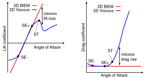
Figure 4.
Notional lift and drag curves of a two-dimensional profile: viscous flow and inviscid flow conditions with flat plate drag correction compared.
Inviscid-flow solutions by BIEM determine blade sectional loads that are consistent with linear relationship between lift and angle of attack and, using the flat-plate analogy in Equation (5) with minimum drag reflecting attached flow conditions (curves in red in Figure 4). The comparison between sectional lift and drag properties motivates the following definition of factors to correct sectional loads by BIEM to represent both attached and separated flow conditions:
where and are, respectively, drag and lift per unit length determined under inviscid 2D flow conditions (i.e., by a 2D BIEM) at angle of attack , while and are profile drag and lift under 2D viscous flow conditions.
Once quantities are known, blade loads correction is obtained through the following procedure. From the BIEM solution, sectional contributions to axial force and tangential force are determined from Equation (3). Next, wake-induced velocity along blade span is determined by taking the gradient of Equation (2) (with ), and the radial distribution of the effective angle of attack is evaluated. Radial distributions of sectional drag and lift follow by projecting force in direction normal and tangent to the effective inflow, as sketched in Figure 3, where is the angular pitch of the blade section at radius r.
Separating pressure-induced and friction-induced contributions to force as defined in Equation (3), lift and drag contributions are also split into pressure-induced and friction-induced terms. Correction factors from Equation (10), yield
where symbol labels viscous-flow corrected quantities. While corrections for pressure-induced lift and friction-induced drag are obvious, the assumption made here is that correction factor for drag can be used to account for flow separation and stall effects on friction-induced lift . Pressure-induced drag correction by stems from the approximated relationship between induced drag and lift that is broadly valid for lifting surfaces. Numerical studies prove that contributions from diagonal terms and are very small as compared to, respectively, contributions .
Converting lift and drag back to respective axial and tangential load components yields quantity that integrated along blade span returns corrected blade axial force, while quantity returns corrected blade torque. Summing over all blades, turbine corrected thrust and torque are obtained (formally, Equation (4) with replaced by ).
A full exploitation of the viscosity correction model described above implies that an iterative procedure is enforced to make the potential flow solution consistent with the modified loading on blades. No iteration has been considered in the present analysis and the subject is briefly address later in Section 6.
3. Case Studies for Validation of Computational Model
Numerical applications of the proposed computational model are discussed by considering two case studies taken from the literature. Both cases address three-bladed model turbines designed for research activity.
For a turbine with radius R, swept area , rotating at angular speed in a current with nominal freestream velocity V, the Tip Speed Ratio (TSR) is defined as
Turbine performance is described through thrust, torque and power coefficients, respectively , defined as
where is the power generated by the turbine.
3.1. Fixed Pitch Turbine
Gaurier et al. [11] describe a 700 mm diameter, fixed-pitch model turbine developed at IFREMER, France. The model has been the subject of the first round-robin test on tidal turbines carried out in the framework of the EU-FP7 MaRINET Project [12], with turbine performance measurements from two towing tanks (Strathclyde University and CNR-INSEAN) and two flume tanks (IFREMER and CNR-INSEAN). Turbine performance curves measured at inflow speed between 0.6 and 1.2 m/s are presented as mean values and standard deviations.
Main turbine geometry parameters are summarized in Table 1. A full description is given in [11]. This testcase is referred to here as the IFREMER-FP turbine.

Table 1.
IFREMER-FP turbine main geometry parameters.
3.2. Variable Pitch Turbine
Bahaj et al. [13] investigate a 800 mm diameter, variable-pitch model turbine developed at the University of Southampton (U.K.). This model was analysed by extensive towing tank and cavitation tunnel tests. Experimental data provide turbine performance at different blade pitch settings, with blades rotated about the spanwise axis over a range of 15 degrees, from to 30°, while is taken as the design condition. This pitch definition refers to the nose-tail angle of the blade at radius . Turbine performance curves are available for inflow speed between 0.8 and 2.0 m/s (cavitation tunnel tests) and between 0.8 and 1.5 m/s (towing tank tests).
Main turbine geometry parameters are summarized in Table 2, while a complete description can be found in [13]. This testcase is referred to here as the UoS-VP turbine.
Table 2.
UoS-VP turbine geometry parameters.
4. Fixed Pitch Turbine Study
The IFREMER-FP turbine performance is analysed with reference to experimental conditions corresponding to the highest inflow speed, m/s. This choice is motivated to avoid a too small Reynolds number characterizing the blade flow. The tip speed ratio is varied between zero and 8. Comparing with the physical model in [11], it may be noted that the stanchion supporting the turbine is not considered in numerical simulations. Similarly, the nacelle portion downstream of the turbine hub is not present in the computational model, see Figure 5.
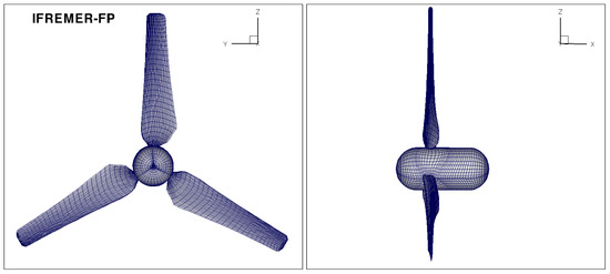
Figure 5.
IFREMER-FP turbine. Computational grid used for calculations by BIEM.
Blade and hub surface discretization parameters are determined as the result of a grid sensitivity study. Each blade is discretized into elements chordwise from leading edge to trailing edge and elements spanwise. Four blade grid levels with and are considered. Hub and wake surface discretizations are built according to blade grid refinement level. Figure 6 presents inviscid-flow thrust and torque predicted by BIEM using the four grids. Three representative TSR values are considered. The torque coefficient evaluated by including the viscous flow correction is also presented to highlight that the VFC model has no effect on the sensitivity of results to grid refinement. From these results it is concluded that a discretization with , is adequate to minimise the effect of further grid refinement on results. In this case, the hub surface is divided into 42 and 54 elements, respectively, in circumferential and longitudinal directions, and the wake is discretized into 36 elements along radius and 60 elements streamwise per revolution. The wake portion considered in the numerical solution of Equation (2) extends for 10 revolutions.
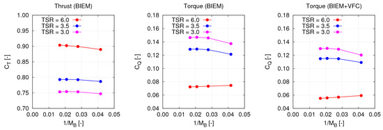
Figure 6.
IFREMER-FP turbine. Calculated thrust and torque coefficients as a function of discretization parameter . Left and center: thrust and torque by non-corrected BIEM; right: torque by BIEM-VFC.
The trailing wake model described in Section 2.1 is used to determine the turbine wake surface. Figure 7 maps the intensity of wake-induced axial velocity evaluated by BIEM at axial locations corresponding to rotor blade trailing edge and at different radial positions over a range of operating conditions identified by the parameter TSR.
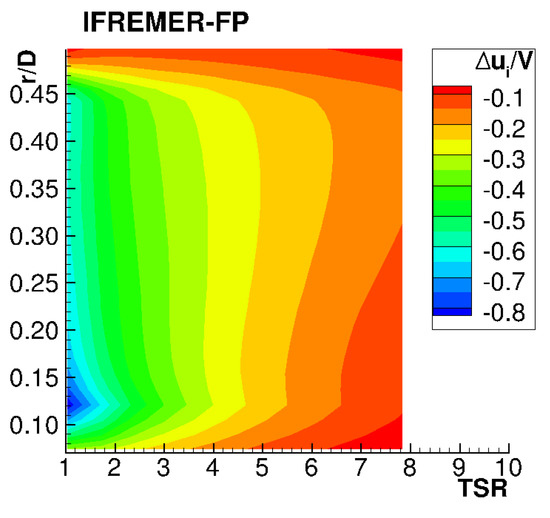
Figure 7.
IFREMER-FP turbine. Calculated axial induced velocity distribution at rotor plane.
The resulting surfaces for three representative values of TSR are shown in Figure 8. The effect of TSR on wake pitch is clear: trailing vortices are rapidly shed away from the rotor at low TSR , while wake spirals pack-up close to the rotor as TSR increases. In all cases, wake pitch increases from inner radii to the tip vortex.
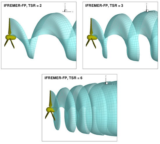
Figure 8.
IFREMER-FP turbine. Trailing wake geometry of BIEM model at different operating conditions: TSR = 2 (top left), TSR = 3 (top right), TSR = 6 (bottom).
Viscous flow effects on blade loads are determined by applying the VFC model described in Section 2.2. The evaluation of correction factors in Equation (11) requires that blade section lift and drag properties are known. For this purpose, the inviscid-flow BIEM solution is used to estimate the local Reynolds number from Equation (6), and the effective angle of attack in Figure 3, at all blade sections for the TSR range from zero to 8 considered in model tests. Results in left Figure 9 show that the local Reynolds number varies between and over most of the TSR range of interest. Right Figure 9 depicts a positive effective angle of attack that increases from values close to zero for the highest TSR to 20–25 degrees for TSR between 1 and 2. At given TSR , both Reynolds and angle of attack present limited variations over a wide blade portion between 30% and 90% of span.
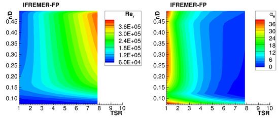
Figure 9.
IFREMER-FP turbine. Reynolds number (left) and effective angle of attack (right) as a function of radius r and of TSR.
Experimental data of lift and drag curves of NACA 63-4xx profiles are available in the literature only at Reynolds number of 10 and higher, which is outside the range of interest in the present analysis as shown above. Lack of experimental data is overcome here by using numerical predictions of polar curves by the X-Foil code [21]. This solver integrates a BIEM for two-dimensional, steady flow with the solution of boundary layer equations in integral form and is largely used in combination with blade element (momentum) methods. The NACA 63-421 profile corresponding to 21% thick blade sections at 70% of span is taken as representative of all blade sections. At angle of attack beyond stall, X-Foil predictions are not reliable and polar curves are completed by the following extrapolation procedure. At very high incidence angles (here, ), lift and drag values are taken from experimental data for the NACA 0015 profile by Sheldahl and Klimas [22]. The assumption is that for very high angles, hydrodynamic loads are weakly sensitive to Reynolds number and to profile shape details. A polynomial fit is used to merge NACA 63-421 data from X-Foil and high angle of attack NACA 0015 data at angle of attack between stall and 30 degrees.
Lift and drag curves calculated by X-Foil are presented in Figure 10. In particular, results for 5 values of Reynolds number are considered in order to adequately describe lift and drag properties over the range of interest (Figure 9 Left). Lift and drag curves from experimental data at 3E6 in [23] are also given for comparison.
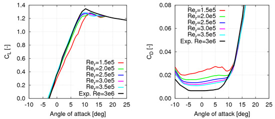
Figure 10.
NACA 63-421 2D foil: lift (left) and drag (right) coefficients calculated by X-Foil and from experiments [23].
Figure 11 maps correction factors along blade span and over the TSR range of interest. Values close to one denote conditions where blade flow is attached or weakly separated and no correction of sectional loads by BIEM is needed. This occurs at TSR ≃ 2.5 and higher, which corresponds to effective angle of attack below 10–12 degrees, as shown in Figure 9. At lower TSR , the effective angle of attack increases up to stall, as apparent from polar curves in Figure 10. As expected, the lift factor drops below 1, while the drag factor rapidly grows, to simulate, respectively, stall-induced lift loss and drag rise.
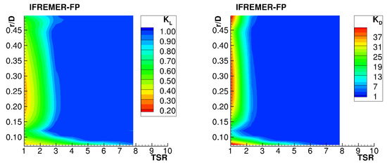
Figure 11.
IFREMER-FP turbine. Correction factors for radial contributions to lift (left) and drag (right) as a function of radius r and of TSR.
Predicted turbine thrust, torque and power curves are presented in Figure 12 and compared with experimental data at m/s from three facilities involved in the round-robin test: CNR-INSEAN towing tank (INSEAN), IFREMER flume tank (IFREMER) and Kelvin Hydrodynamics Laboratory at University of Strathclyde (KHL). Results from the fourth facility participating to the round robin test, CNR-INSEAN flume tank, are omitted here since they fall within the range given by those considered in plots. For the sake of precision, measured thrust and power coefficients only are presented in [11]. Here, also the torque coefficient is considered because this quantity provides a direct indication of the accuracy of blade tangential forces evaluated by the numerical model.
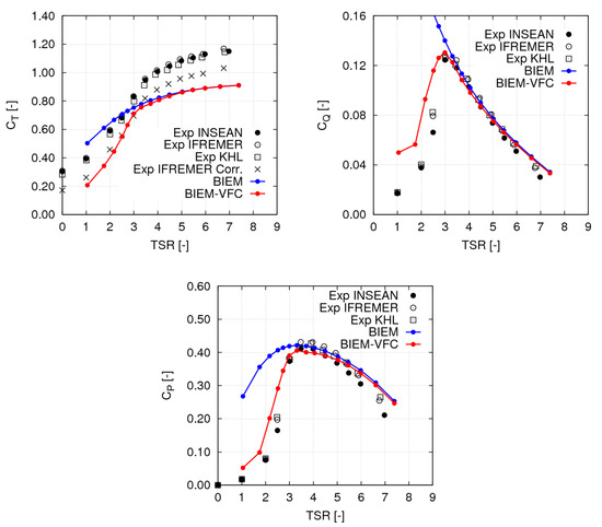
Figure 12.
IFREMER-FP turbine performance predictions by BIEM and BIEM-VFC compared to experimental data in [11]: thrust (top left); torque (top right) and power (bottom) coefficients.
It is important to observe that present experimental and numerical results use different definitions of thrust and torque. Numerical thrust and torque are determined by integrating hydrodynamic loads on blade surfaces, while in the experimental set-up, turbine torque denotes the axial moment measured by a torque sensor placed between the rotating hub and the fixed nacelle. Assuming the contribution to torque of the rotating hub is negligible, numerical and experimental data are consistent. Both numerical and experimental power are evaluated from the hydrodynamic torque Q as .
Less direct is the comparison between numerical and measured thrust. Turbine thrust reported in [11] denotes the axial force at the top of the mast supporting the turbine. This quantity combines blades thrust with a non negligible resistance contribution from hub, nacelle and the mast piercing the free surface. Tests performed at IFREMER of a dummy IFREMER-FP rotor with no blades determined at m/s (not reported in [11]). For the sake of completeness, top left Figure 12 also presents measured axial force with the contribution subtracted. This result is referred to as ’Exp IFREMER Corr.’.
Numerical results in Figure 12 include both BIEM without viscosity correction and corrected values by Equation (11) (label BIEM-VFC). As expected from the discussion above, viscosity effects are negligible at TSR = 5 and higher, while small differences between standard BIEM (that is, with non viscous flow corrections) and BIEM-VFC predictions are noted for TSR . In this range, numerical and experimental results for torque and power are in good agreement, while thrust is underestimated in numerical results. The reason for this difference in thrust is not clear and could be related to hub, nacelle and mast resistance contributions that are only approximately subtracted from axial force measurements.
At TSR lower than 3, massive flow separation and stall determine a dramatic reduction of thrust, torque and power that is missed in standard BIEM results, while BIEM-VFC results capture the correct trend. In particular, measured peak values of and are matched at the correct TSR values. At very low TSR , where deep stall conditions occur on blades, the BIEM-VFC model overpredicts both torque and power, but the viscous flow correction allows to recover most of the error affecting inviscid-flow predictions by non-corrected BIEM.
Figure 13 and Figure 14 address blade pressure distributions evaluated by BIEM. Specifically, the pressure coefficient is defined as
where the pressure p is evaluated by BIEM and is the velocity of the flow incoming to the blade section at radius r. Recalling that the VFC model applies only to global loads and not to the pressure distribution, calculated is representative only in the TSR range where viscosity correction is not significant. For the present case, this approximately holds for TSR . Figure 13 depicts pressure distributions on blades pressure and suction sides at TSR = 3.3 (peak power condition, see Figure 12). The effect of TSR on blade pressure distribution is illustrated in Figure 14, where along the blade section at for four values of TSR is plotted. As expected, the pressure jump between pressure and suction sides tends to reduce as TSR is increased from the peak power condition.

Figure 13.
IFREMER-FP turbine. Pressure distribution evaluated by inviscid-flow BIEM, TSR = 3.3 (peak power condition). Left: pressure side; right: suction side.
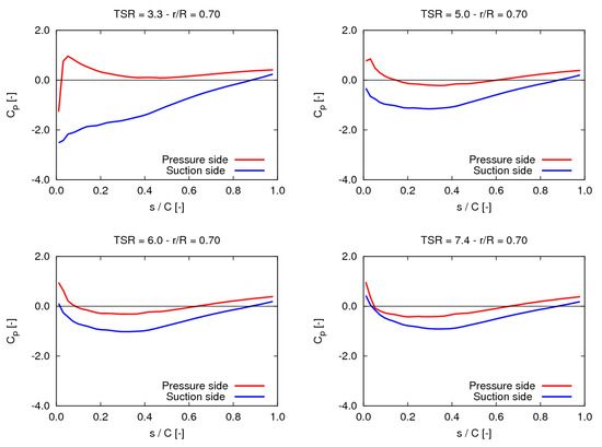
Figure 14.
IFREMER-FP turbine. Pressure distribution evaluated by inviscid-flow BIEM at radial section at 70% of blade span. From top left to bottom right: TSR = 3.3, 5, 6, 7.4.
5. Variable Pitch Turbine Study
The variable-pitch UoS-VP turbine described in Bahaj et al. [13] represents a valuable benchmark to investigate the capability of a computational model to capture the effect of blade pitch variations on turbine loads and in particular to correctly describe performance in off-design conditions. As for the fixed-pitch IFREMER-FP turbine discussed above, a simplified three-dimensional model is used in which the aft portion of the nacelle and the supporting stanchion are omitted. Another difference exists at blade root where NACA 63-8xx sections are used in the computational model, while the physical model presents cylindrical sections to actuate pitch variations. Figure 15 shows the computational grid built for BIEM calculations. Discretization parameters are similar to the IFREMER-FP case.
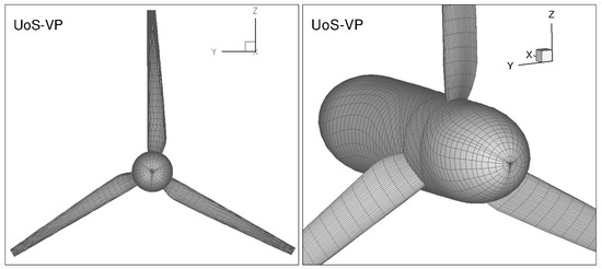
Figure 15.
UoS-VP turbine. Three-dimensional model and computational grid for BIEM analysis. Left: front view; right: details of hub and blade roots.
Figure 16 depicts the intensity of wake-induced velocity from Equation (7) evaluated by BIEM at axial locations corresponding to rotor blade trailing edge and 70% of blade span. Different blade pitch settings and a range of operating conditions corresponding to model tests are plotted. For a given value of TSR the intensity of the induced velocity increases with the blade pitch setting. It should be noted that for the lowest pitch angle case the calculated value of the normalised induced velocity tends to exceed the theoretical limit at the rotor plane given by the Betz theory.
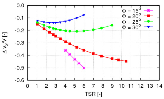
Figure 16.
UoS-VP turbine. Axial induced velocity distribution at axial position corresponding to blade trailing edge and 70% of blade span. Different pitch settings compared.
The resulting trailing wake surfaces for the design condition and for three representative values of TSR are shown in Figure 17.
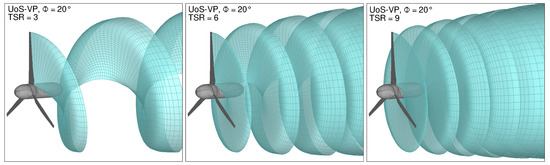
Figure 17.
UoS-VP turbine. Wake geometry of BIEM model at different operating conditions. From left to right, TSR = 3, 6, 9. Design pitch setting, .
Turbine operating conditions considered in the present analysis refer to selected cavitation tunnel test conditions from [13] as summarized in Table 3.
Table 3.
UoS-VP turbine. Inflow speed conditions.
Recalling Equation (6), Reynolds number characterizing blade section flow at radius r depends on the inflow velocity V. Figure 18 maps its distribution as a function of radius and TSR for pitch setting , while Figure 19 compares at 70% of blade span for the highest and lowest inflow speed cases from Table 3. Results indicate that approximately varies between and over most of the operating range of interest here.
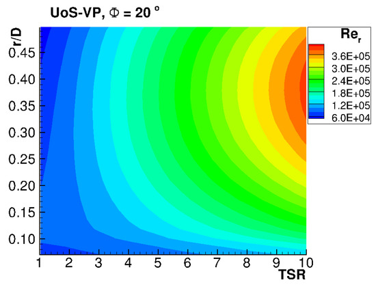
Figure 18.
UoS-VP turbine. Reynolds number as a function of radius r and of turbine operating condition (TSR).
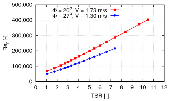
Figure 19.
UoS-VP turbine. Reynolds number at radius for pitch settings corresponding to the highest inflow speed ( m/s, ), and for the lowest inflow speed ( m/s, ).
The effective angle of attack evaluated by standard BIEM is presented in Figure 20. Specifically, distributions along blade span at variable TSR are presented for design pitch setting, , and Figure 21 presents the variability of this quantity at different pitch settings at 70% of blade span. Case shows blade sections mostly operating in the range with higher values only at TSR . As expected, larger pitch angles determine lower values.
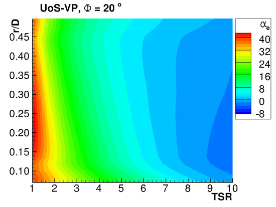
Figure 20.
UoS-VP turbine. Effective angle of attack as a function of radius r and of turbine operating condition (TSR). Design pitch setting .
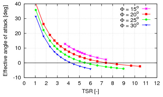
Figure 21.
UoS-VP turbine. Effective angle of attack at radius for different pitch settings and TSR.
Reference [24] provides lift and drag curves of the NACA 63-815 foil at . This 15% thick foil is taken as representative of UoS-VP turbine sections whose thickness ratio varies from 0.176 at 50% of span to 0.126 at tip. Recalling Figure 18 and Figure 19, is higher than the range of interest in the present analysis. In order to obtain lift and drag data in the actual and ranges, the X-Foil code is used and 6 polar curves for are evaluated. Polar data are completed at very high angle of attack using NACA 0015 profile data and polynomial interpolation as described in Section 3.2 for the IFREMER-FP turbine. Resulting lift and drag curves are plotted in Figure 22 and experimental data from [24] are also shown for comparison. Lift curves show that stall conditions are predicted by X-Foil at about 10–12 degrees, while experimental data show a more gradual transition to stall between 8 and 12 degrees. Results for drag are in agreement only at negative angle of attack, while experimental data present quite larger values than X-Foil between 2 and 12 degrees. These discrepancies cannot be explained because of the different numbers in the two datasets. Furthermore, drag measurements also show a large scatter.
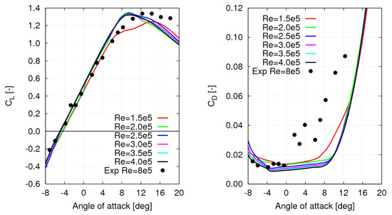
Figure 22.
NACA 63-815 2D foil: lift (left) and drag (right) coefficients used for the viscous flow correction of BIEM.
Lift and drag properties predicted by X-Foil are used to feed the viscous flow correction model described in Section 2.2. Contour maps in Figure 23 show and factors for design pitch setting , while Figure 24 depicts the variation of these quantities at over the pitch settings range. In case , viscosity effects on blade section lift and drag are negligible at TSR of about 3.5–4 and higher, which corresponds to non-separated flow conditions at angle of attack below 8–10 degrees, see Figure 20 and Figure 22. At lower TSR , the lift correction factor gradually decreases to about 0.3 (lift loss under stall) while the drag correction factor suddenly increases to values of 30 and more (drag crisis).
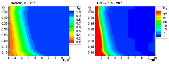
Figure 23.
UoS-VP turbine. Correction factors for radial contributions to lift (left) and drag (right) as a function of radius r and of operating condition (TSR). Pitch setting .
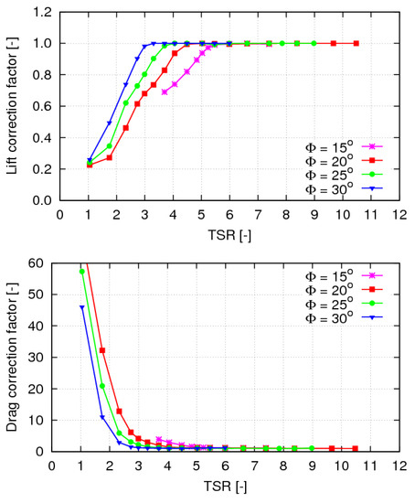
Figure 24.
UoS-VP turbine. Lift correction factor (top) and drag correction factor (bottom) at radius for different Pitch settings.
Consistent with sectional angle of attack values commented above, pitch settings limit flow separation and stall effects to very low values of TSR , while in case , most of the addressed operating range is under the effect of flow separation and stall.
Turbine thrust and power predictions by BIEM and by BIEM-VFC using blade section polar data from X-Foil are compared with model test measurements from [13] in Figure 25 and Figure 26. In general, it may be noted that standard BIEM predictions of both thrust and power fairly reproduce experimental data only in the high TSR range for pitch setting cases . For operating conditions corresponding to peak power TSR and lower values of TSR , standard BIEM results overpredict both thrust and power, since the effects of blade flow separation and stall are not captured. When the VFC model is applied to correct BIEM, predicted thrust and power of cases are in fair agreement with measured data over a full TSR range. For extreme off-design cases and , large differences between numerical and experimental results are observed even if the viscous flow correction is applied. In particular, at predicted presents an unphysical trend with increasing TSR . A possible explanation for this result is that under extreme off-design conditions, blade flow is affected by a complex separated flow phenomenology that is beyond the limits of the proposed VFC model, and a detailed CFD analysis would be necessary. Unfortunately, experimental data do not give information at very low TSR where deep-stall conditions are expected. Large scattering of measured thrust and power is also noted in extreme off-design conditions.
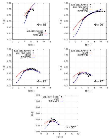
Figure 25.
UoS-VP turbine performance predictions by BIEM and BIEM-VFC compared to experimental data in [13]. Thrust coefficient at pitch settings .
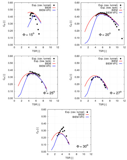
Figure 26.
UoS-VP turbine performance predictions by BIEM and BIEM-VFC compared to experimental data in [13]. Power coefficient at pitch settings .
The capability of the BIEM-VFC model to correctly describe turbine performance trends at different pitch settings can be discussed considering results in Figure 27, where four performance indicators are considered: maximum value of thrust coefficient , maximum value of power coefficient , and corresponding values of TSR where maxima are established (labelled, respectively, as TSR@, and TSR@). Numerical predictions by BIEM-VFC and polar data from X-Foil (label: VFC, XFOIL Polar) are compared with polynomial fits of experimental data from cavitation tunnel tests as presented in Figure 7 of [13] (label: Model tests). Numerical results by BIEM-VFC using experimental data for blade section lift and drag taken from measurements in [24] are also presented (label: VFC, Exp. Polar).
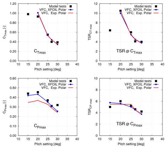
Figure 27.
UoS-VP turbine. Effect of pitch setting : from top to bottom, left to right, and corresponding TSR values TSR@, TSR@.
Quantity by BIEM-VFC and X-Foil and the corresponding TSR values fairly reproduce the trend observed in experiments over the range . Similar comments can be made for the maximum power except for case , where predicted is some 20% lower than measured. However, fitted experimental data at show a rather inconsistent trend with . At off-design pitch , BIEM-VFC and X-Foil results match experimental data for and the corresponding TSR , while the prediction is not plotted since numerical results show an unphysical trend with increasing TSR as already discussed.
Figure 27 allows to compare BIEM-VFC results based on X-Foil predictions of sectional lift and drag properties with those obtained by considering measured lift and drag in [24]. As already commented in Figure 22, measured drag is much higher than X-Foil predictions over a significant range of angle of attack. As expected, this results in underestimation of turbine power coefficient, bottom left Figure 27. Smaller differences between measured and X-Foil lift observed in left Figure 22, have a negligible effect on predicted turbine thrust coefficient, as shown in top Figure 27.
In order to complete the present validation study, it is also interesting to compare results by the proposed BIEM-VFC approach with data from the literature obtained using different computational models. Two cases are considered here: Bahaj et al. [25] present results by two solvers based on Blade Element Method (BEM) for pitch settings from to . Next, Baltazar and Falcão de Campos [7] present results by BIEM with viscous flow corrections for cases , and 27°.
For the sake of clarity, comparisons with BEM and BIEM results from the literature are presented in different figures. Thrust and torque coefficient predictions by the present BIEM-VFC model are compared with results by BEM [25] in Figure 28 and Figure 29. Results by BEM solvers GH-Tidal and SERG-Tidal show an accuracy with respect to model test results in [13] that is broadly comparable to what is obtained using the present BIEM-VFC. Predictions by BIEM-VFC and GH-Tidal are closer to experiments than SERG-Tidal for pitch settings , while the opposite holds for . This trend is only in part confirmed in Figure 29 where power coefficient results are shown. While BIEM-VFC and SERG-Tidal show a comparable accuracy for at , results by GH-Tidal overestimate experimental data. It is also noted that off-design case shows similar results between BEM and the present BIEM-VFC for the thrust coefficient, while power coefficient results are very different, with BEM models fairly capturing power peak and failing to predict results at higher TSR.
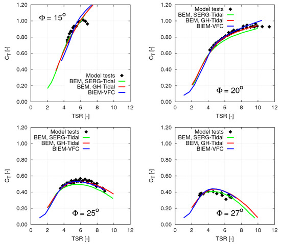
Figure 28.
UoS-VP turbine performance predictions by BIEM-VFC compared to results of BEM models from [25]: thrust coefficient . Pitch settings to 27°.
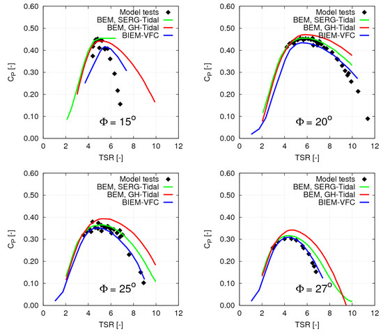
Figure 29.
UoS-VP turbine performance predictions by BIEM-VFC compared to results of BEM models from [25]: power coefficient . Pitch settings to 27.
Comparisons between the present BIEM-VFC model and the BIEM with viscous flow correction proposed in [7] are presented in Figure 30. In general, the agreement of the two numerical models with experimental data is comparable with some exceptions. Results by the present BIEM-VFC model better reproduce measured turbine power in case and thrust in case , while results from [7] better predict thrust in case . In these cases, differences occur throughout the TSR range and hence they can be explained as a combined effect of different viscosity correction and trailing wake models in the two formulations.
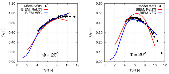
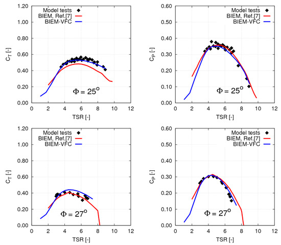
Figure 30.
UoS-VP turbine performance predictions by BIEM-VFC compared to results from the BIEM model in [7]: thrust coefficient (left); and power coefficient (right). Pitch settings to 27°.
6. Discussion
The analysis of present results compared to reference data from the literature highlights the importance of adding a viscous flow correction to standard BIEM results obtained under inviscid-flow assumptions. Although simple and partially based on semi-empirical corrections, the proposed BIEM-VFC approach allows to significantly improve the reliability of turbine performance predictions by BIEM over a full range of operating conditions, including design and off-design blade pitch settings.
The main advantage of BIEM modelling compared to blade element momentum methods routinely used for marine turbines is the possibility to determine a consistent representation of the three-dimensional flow around rotor blades and hub in steady or unsteady flow. Pressure distributions on the blade surface can be used as input to predict the occurrence of cavitation and to estimate its detrimental effects in terms of vibrations, noise, erosion.
Nonetheless, a major weakness of the present BIEM-VFC approach is that viscosity correction applies only to blade loads and not to the potential flow solution as a whole. In particular, the correction does not apply to the intensity of the vortex sheet shed at blade trailing edge, nor to the induced velocity field necessary to evaluate the effective angle of attack. Neglecting these effects is expected to be the source of errors in performance predictions when the turbine operates at TSR lower than the peak power condition.
To overcome this limitation, a generalization of the present VFC model is the subject of work underway. Specifically, trailing vorticity distributions that are compatible with the correction of blade loads determined by the VFC scheme described in Section 2.2 can be obtained through an iterative procedure in which the direct relationship between axial and tangential force contributions by a blade element at radius r and turbine-induced velocity perturbation is derived by momentum and moment of momentum balance. Furthermore, the boundary integral representation (2) is generalised to include additional source terms according to the viscous/inviscid coupling methodology proposed in [26].
In addition to single turbine performance studies, the BIEM-VFC methodology is also applied to study the hydrodynamic behaviour of turbines operating in arrays. In this case, the inviscid-flow BIEM with VFC model is combined with a viscous flow solver (Reynolds-Averaged Navier-Stokes, RANS) to correctly describe the turbulent, vortical stream that characterizes the inflow to a turbine in the wake of similar devices placed upstream. An application of this combined BIEM-VFC and RANS computational methodology has been discussed by the authors in [27], where the interaction between two three-bladed turbines axially aligned with the upstream flow is analysed and numerical results are compared with experimental data from [28].
7. Conclusions
A computational methodology for the hydrodynamic analysis of horizontal axis marine current turbines has been presented, and results of a validation study have been discussed. The approach is based on a Boundary Integral Equation Model (BIEM) for inviscid flows that is combined with a trailing wake model specific for hydrokinetic turbines and with a viscous flow correction model (VFC) to include blade flow separation and stall effects on predicted hydrodynamic loads. The latter is derived by a semi-empirical approach in which inviscid-flow blade loads by BIEM are corrected on the basis of lift and drag properties of two-dimensional foils describing blade sections under equivalent three-dimensional flow conditions.
Numerical predictions by BIEM-VFC have been validated through comparisons with experimental data and with numerical results from the literature. The analysis highlights the capability of the proposed methodology to correctly describe turbine performance over a full range of operating conditions. Specifically, reliable predictions of turbine thrust, torque and power are obtained at medium/high tip speed ratio regimes, where blade flow is mostly attached, but also at relatively low tip speed ratio, where blade flow separation and stall determine thrust loss and drag crisis. More in details, good predictions of turbine performance are obtained for blade pitch settings close to design, while discrepancies for both thrust and torque (power) are observed in off-design conditions.
Comparing BIEM-VFC with other computational models in the literature, a key finding is that the accuracy of the proposed approach is aligned with blade element methods that are routinely used for the analysis and design of marine as well as wind turbines. Such a result is particularly important in that the present methodology based on BIEM provides a physically consistent description of the three-dimensional flow around a turbine in arbitrary onset flow, while blade element methods rely on taylored, case-dependent corrections for blade tip effects, for blade/hub interaction, number of blades. Well known limitations of blade element methods to analyse non-uniform flow conditions as well as to study turbine cavitation are also overcome through the more general description of turbine flow obtained by a BIEM approach.
Future work will address the generalization of the present VFC scheme to achieve trailing vorticity distributions and induced velocity distributions that are fully consistent with the viscosity correction applied on blade loads. Further validation studies will focus on the capability of the generalised BIEM-VFC model to predict turbine performance at low TSR and when turbine blades operate in off-design conditions.
Author Contributions
F.S. and Z.S. developed the original viscous flow correction and trailing wake models while D.C. and F.S. adapted the existing BIEM model. Z.S. and F.S. were responsible for computational model validation studies. All the authors contributed to results analysis and discussion.
Acknowledgments
The work described has been funded under the CNR-INSEAN Project ULYSSES (Underpinning LaboratorY for Studies on Sea Energy Systems). The authors wish to thank Benoit Gaurier for his kind support in the analysis of validation data from experiments at IFREMER. Part of validation data have been developed under the EU-FP7 MaRINET Project (Grant 262552).
Conflicts of Interest
The authors declare no conflict of interest.
Nomenclature
| Symbol | Description | Units |
| c | Turbine blade chord | [m] |
| Pressure coefficient | [-] | |
| Power coefficient | [-] | |
| Friction coefficient | [-] | |
| Torque coefficient | [-] | |
| Thrust coefficient | [-] | |
| D | Turbine diameter, | [m] |
| D | Drag | [N] |
| Drag correction factor | [-] | |
| Lift correction factor | [-] | |
| L | Lift | [N] |
| n | Turbine rotational speed | [s] |
| P | Turbine power | [W] |
| Reference pressure | [Pa] | |
| Q | Turbine torque | [Nm] |
| R | Turbine radius | [m] |
| Reynolds number, Equation (6) | [-] | |
| T | Turbine thrust | [N] |
| TSR | Tip Speed Ratio | [-] |
| V | Freestream velocity | [ms] |
| angle of attack | [deg] | |
| Kynematic viscosity | [ms] | |
| Velocity scalar potential | [ms] | |
| Turbine rotational speed | [rads] | |
| Wake (linear) pitch | [m] | |
| Blade pitch | [deg] | |
| Water density | [kgm] |
References
- Hansen, M.O.L. Aerodynamics of Wind Turbines, 2nd ed.; Earthscan: London, UK, 2008. [Google Scholar]
- Buhl, M.L., Jr. A New Empirical Relationship between Thrust Coefficient and Induction Factor for the Turbulent Windmill State; Technical Report NREL/TP-500-36834; National Renewable Energy Laboratory: Golden, CO, USA, 2005.
- Shen, W.Z.; Mikkelsen, R.; Sœrensen, J.N.; Bak, C. Tip Loss Corrections for Wind Turbine Computations. Wind Energy 2005, 8, 457–475. [Google Scholar] [CrossRef]
- Young, Y.L.; Motley, M.R.; Yeung, R.W. Three-Dimensional Numerical Modeling of the Transient Fluid-Structural Interaction Response of Tidal Turbines. J. Offshore Mech. Arct. Eng. 2010, 132, 1–12. [Google Scholar] [CrossRef]
- He, L.; Xu, W.; Kinnas, S.A. Numerical Methods for the Prediction of Unsteady Performance of Marine Propellers and Turbines. In Proceedings of the ISOPE 2011 Twenty-First International Offshore and Polar Engineering Conference, Maui, HI, USA, 19–24 June 2011. [Google Scholar]
- Baltazar, J.; Falcão de Campos, J.A.C. Unsteady Analysis of a Horizontal Axis Marine Current Turbine in Yawed Inflow Conditions With a Panel Method. In Proceedings of the SMP’09 First International Symposium on Marine Propulsors, Trondheim, Norway, 22–24 June 2009; Koushan, K., Steen, S., Eds.; MARINTEK (Norwegian Marine Technology Research Institute): Trondheim, Norway, 2009. [Google Scholar]
- Baltazar, M.J.; Falcão de Campos, J.A.C. Hydrodynamic design and analysis of horizontal axis marine current turbines with lifting line and panel methods. In Proceedings of the OMAE2011 ASME 30th International Conference on Ocean, Offshore and Arctic Engineering, Rotterdam, The Netherlands, 19–24 June 2011; The American Society of Mechanical Engineers: Rotterdam, The Netherlands, 2011; Volume 5, pp. 453–465. [Google Scholar]
- Salvatore, F.; Testa, C.; Greco, L. A Viscous/Inviscid Coupled Formulation for Unsteady Sheet Cavitation Modelling of Marine Propellers. In Proceedings of the CAV 2003 Fifth International Symposium on Cavitation, Osaka, Japan, 1–4 November 2003. [Google Scholar]
- Salvatore, F.; Greco, L.; Calcagni, D. Computational analysis of marine propeller performance and cavitation by using an inviscid-flow BEM model. In Proceedings of the SMP’11 Second International Symposium on Marine Propulsion, Hamburg, Germany, 15–17 June 2011. [Google Scholar]
- Pereira, F.; Salvatore, F.; Di Felice, F. Measurement and Modelling of Propeller Cavitation in Uniform Inflow. J. Fluids Eng. 2004, 126, 671–679. [Google Scholar] [CrossRef]
- Gaurier, B.; Germain, G.; Facq, J.-V.; Johnstone, C.M.; Grant, A.D.; Day, A.H.; Nixon, E.; Di Felice, F.; Costanzo, M. Tidal energy Round Robin tests: Comparisons between towing tank and circulating tank results. Int. J. Mar. Energy 2015, 12, 87–109. [Google Scholar] [CrossRef]
- EU-FP MaRINET Project. Available online: https://cordis.europa.eu/project/rcn/98372_en.html (accessed on 29 March 2018).
- Bahaj, A.S.; Molland, A.F.; Chaplin, J.R.; Batten, W.M.J. Power and thrust measurements of marine current turbines under various hydrodynamic flow conditions in a cavitation tunnel and a towing tank. Renew. Energy 2007, 32, 407–426. [Google Scholar] [CrossRef]
- Morino, L. Boundary Integral Equations in Aerodynamics. Appl. Mech. Rev. 1993, 46, 445–466. [Google Scholar] [CrossRef]
- Greco, L.; Salvatore, F.; Di Felice, F. Validation of a Quasi—Potential Flow Model for the Analysis of Marine Propellers Wake. In Proceedings of the ONR-2004 Twenty-fifth ONR Symposium on Naval Hydrodynamics, St. John’s, NL, Canada, 8–13 August 2004; National Academies Press: Washington, DC, USA, 2004. [Google Scholar]
- Carlton, J.S. Marine Propellers and Propulsion, 1st ed.; Butterworth–Heinemann: Oxford, UK, 1994. [Google Scholar]
- Betz, A. The Maximum of the Theoretically Possible Exploitation of Wind by Means of a Wind Motor. Wind Eng. 2013, 37, 441–446, (Translation by Hamann et al. of original paper published in 1920 by the author in German). [Google Scholar] [CrossRef]
- Okulov, V.L.; Sørensen, J.N. Maximum efficiency of wind turbine rotors using Joukowsky and Betz approaches. J. Fluid Mech. 2010, 649, 497–508. [Google Scholar] [CrossRef]
- Micek, P.; Gaurier, B.; Germain, G.; Pinon, G.; Rivoalen, E. Experimental study of the turbulence intensity effects on marine current turbines behaviour. Part I: One single turbine. Renew. Energy 2014, 66, 729–746. [Google Scholar] [CrossRef]
- Del Frate, C.; Di Felice, F.; Alves Pereira, F.; Romano, G.P.; Dhomé, D.; Allo, J.-C. Experimental Investigation of the turbulent flow behind a horizontal axis tidal turbine. In Progress in Renewable Energies Offshore, Proceedings of the RENEW 2016 2nd International Conference on Renewable Energies Offshore, Lisbon, Portugal, 24–26 October 2016; CRC Press: Boca Raton, FL, USA, 2016. [Google Scholar]
- Drela, M. XFOIL: An Analysis and Design System for Low Reynolds Number Airfoils. In Low Reynolds Number Aerodynamics, Proceedings of the Conference Notre Dame, IN, USA, 5–7 June 1989; Lecture Notes in Engineering, Bd. 54; Springer: Berlin/Heidelberg, Germany, 1989; pp. 1–12. ISBN 978-3-540-51884-6. [Google Scholar]
- Sheldahl, R.E.; Klimas, P.C. Aerodynamic Characteristics of Seven Symmetrical Airfoil Sections Through 180-Deg. Angle of Attack for Use in Aerodynamic Analysis of Vertical Axis Wind Turbines; Technical Report SAND80-2114; SANDIA: Albuquerque, NM, USA, 1981. [Google Scholar]
- Abbott, I.R.; von Doenhoff, A.E. Summary of Airfoil Data; NACA Report 824; NACA: Boston, MA, USA, 1945. [Google Scholar]
- Molland, A.F.; Bahaj, A.S.; Chaplin, J.R.; Batten, W.M.J. Measurements and predictions of forces, pressures and cavitation on 2D sections suitable for marine current turbines. J. Eng. Marit. Environ. 2004, 218, 127–138. [Google Scholar]
- Bahaj, A.; Batten, W.; McCann, G. Experimental verifications of numerical predictions for the hydrodynamic performance of horizontal axis marine current turbines. Renew. Energy 2007, 32, 2479–2490. [Google Scholar] [CrossRef]
- Morino, L.; Salvatore, F.; Gennaretti, M. A New Velocity Decomposition for Viscous Flows: Lighthill’s Equivalent-Source Method Revisited. Comput. Methods Appl. Mech. Eng. 1999, 173, 317–336. [Google Scholar] [CrossRef]
- Salvatore, F.; Calcagni, D.; Sarichloo, Z. Development of a Viscous/Inviscid Hydrodynamics Model for Single Turbines and Arrays. In Proceedings of the EWTEC 2017 Twelfth European Wave and Tidal Energy Conference, Cork, Ireland, 27 August–1 September 2017. [Google Scholar]
- Mycek, P.; Gaurier, B.; Germain, G.; Pinon, G.; Rivolaen, E. Experimental Study of the Turbulence Intensity Effects on Marine Current Turbines Behaviour. Part II: Two Interacting Turbines. Renew. Energy 2014, 68, 876–892. [Google Scholar] [CrossRef]
© 2018 by the authors. Licensee MDPI, Basel, Switzerland. This article is an open access article distributed under the terms and conditions of the Creative Commons Attribution (CC BY) license (http://creativecommons.org/licenses/by/4.0/).