Implementation of an Implicit Solver in ADCIRC Storm Surge Model


1
Department of Electrical and Computer Engineering, Tennessee State University, Nashville, TN 37209, USA
2
Department of Mechanical and Manufacturing Engineering, Tennessee State University, Nashville, TN 37209, USA
*
Author to whom correspondence should be addressed.
J. Mar. Sci. Eng. 2018, 6(2), 62; https://doi.org/10.3390/jmse6020062
Submission received: 30 April 2018
/
Revised: 24 May 2018
/
Accepted: 25 May 2018
/
Published: 1 June 2018
Abstract
:The current state of science does not offer any remedy to stop a hurricane from occurring. Therefore, accurate storm surge models capable of predicting water velocity and elevation are indispensable. In this paper, the implementation of an implicit solver in the Advanced Circulation (ADCIRC) storm surge model is presented. The implemented implicit solver uses hybrid finite element and finite volume techniques for solving shallow water equations. Objectives of this research include: Enhancing numerical stability, providing an option of using large timesteps, and the usage of a relatively easier mathematical formulation than the existing one in ADCIRC. The storm surge hindcast of Hurricane Katrina that hit Louisiana and Mississippi in 2005 is used as a case study. Stability of the solver, comparison of water elevation and velocity against observed data, impact of timestep sizes, and execution times of solvers are thoroughly investigated in this study. Results of the implemented implicit solver are compared with those of existing lumped explicit and semi-implicit solvers of ADCIRC; the findings appear to be very promising.
1. Introduction
Hurricanes are among the worst natural disasters, and storm surges caused by these hurricanes are the deadliest and most egregious contributors to the resulting destruction. Even though it is not the only factor, climate change has made the impact of hurricanes much worse than ever [1]. Hurricanes have many aspects that need to be investigated; however, this paper focuses only on the modeling of storm surges that hurricanes bring to land. To address this global challenge, the need for precise, fast, and reliable models that are capable of predicting storm surges, floods, and levee overtopping is indispensable. The physics of ocean circulation and the impact of hurricanes on ocean shallow water are formulated mathematically in the Shallow Water Equations (SWEs), and computer programs, called storm surge models, are used to numerically solve these equations. The simulation of the phenomena is performed days before an impending hurricane hits the coast to predict the water surge elevation and velocity. The algorithms used to solve the SWEs equations depend on explicit [2], semi-implicit [2], or implicit [3] methods. Since today’s scientific status quo does not offer any remedy to stop hurricanes from occurring, accurate predictions of the storm surge would have significant impact on evacuation planning and execution that should potentially lessen damages. Wrongful predictions may result in unpreparedness for disasters, or unnecessary preparedness that would diminish public trust in authorities.
Advanced Circulation (ADCIRC) [4] framework is a well-known model used by the U.S. government and many research and insurance entities to predict or study storm surges in coastal regions. However, due to its explicit or semi-implicit method of solving the SWEs, the stability of this model may be a matter of concern in shallow water regions, especially when large timesteps are used [5].
In this paper, the implementation of an implicit solver, called Computation and Modeling Engineering Laboratory (CaMEL) [3], is performed in the ADCIRC framework. Implicit solvers are inherently more stable than typical explicit or semi-implicit solvers, and hence are capable of entertaining large timesteps [5]. Objectives of implementing the implicit solver in ADCIRC are to enhance the numerical stability, provide an option of using large timesteps, take advantage of the efficient parallel architecture of the ADCIRC framework, and reduce the complexity of the mathematical formulation that currently exists in ADCIRC. The Generalized Wave Continuity Equation formulation of ADCIRC requires some manipulation of the primitive continuity equation that involves adding the time derivative of the continuity equation and subtracting the gradient of vertically integrated momentum equations with it [2,6]. This manipulation is needed to avoid spurious oscillations in water elevation; however, it inadvertently adds some complexity in the mathematical formulation of the ADCIRC model. On the other hand, CaMEL keeps the mathematical formulation as close as possible to the fundamental conservation equations [3,5,7], which may be a matter of great advantage to model developers and users. Note that the scope of this paper is limited to the implementation of an implicit solver in the ADCIRC model, and it does not address any accuracy or reliability issues that may already have had existed in the ADCIRC framework.
2. Governing Equations
The implemented CaMEL implicit solver was originally presented by Akbar and Aliabadi [3] and Aliabadi et al. [7]. This solver uses hybrid finite element and finite volume methods to solve the shallow water equations to model hurricane storm surges. The SWEs are a set of parabolic partial differential equations that describe the flow below a pressure surface in a fluid, which is influenced by several forces including wind field, rotation of the earth, tidal forces, bottom frictions, etc. The SWEs can be derived by depth-averaging the Navier-Stokes equations for a column of fluid with mass and momentum conservation. The scale of length in a horizontal plane is much greater than the scale of length in a vertical plane. In SWEs, the vertical velocity of fluid is negligible due to mass conservation, and vertical pressure is hydrostatic, which results in a homogenous flow along the vertical axis. The velocity and depth of fluid moving in the domain with boundary during the time interval can be described in non-conservation form by the followings:
where h, H, , , , , , , , and are water hydrodynamic head, water depth, net source term, velocity vector, water density, atmospheric pressure on the surface, ocean bottom elevation, earth tidal potential reduction factor, tidal internal forcing water elevation, kinematic viscosity of water, and Coriolis force, respectively [5]. More details about the Coriolis forces, tidal forcing, bottom friction and wind stress terms, can be found in References [8,9,10,11].
The CaMEL solver uses a non-dimensional form of the conservation equations, which is manipulated to a predictor-corrector formulation [5]. The predictor equation is a modified momentum equation to solve for velocity and can be written in accordance to the finite volume formulation as the following,
where M and S are given, as
The corrector equation is a modified continuity equation and can be written in accordance to the finite element formulation for all and such that:
where
3. Methodology
In this study, Hurricane Katrina storm surge hindcast is used for all the numerical experiments presented below to assure the consistency between the ADCIRC lumped explicit, semi-implicit, and the newly implemented implicit solvers. The simulation of hurricane Katrina starts at midnight on 27 August 2005 UTC and ends at 6:00 a.m. on 31 August 2005 UTC with a total time of 4.208 days. For the wind data, the best track data published by the National Oceanic and Atmospheric Administration (NOAA) is used as an input to ADCIRC [16] using ‘NWS’ input option ‘4′ after producing wind field using Planetary Boundary Layer (PBL) model (‘p15′ compiled in ADCIRC ‘work’ folder). A mesh, called EC2001, is used here, which covers the Gulf of Mexico and a large part of the Atlantic Ocean consisting of 254,565 nodes and 492,179 elements, which is the same mesh used by Mukai et al. to derive the ADCIRC tidal database for the United States east coast [17]. The Renaissance Computing Institute (RENCI) [18], which is one of the high-performance computing (HPC) facilities that ADCIRC developers use for live forecasting, is used for all experiments presented here. RENCI HPC environment consists of a cluster of Dell blade servers with two 8-core Intel Xeon E5 processors connected by InfiniBand FDR/Ethernet 10/40GB interconnect [19]. A total of 128 processors are used in all experiments below unless stated otherwise. Note that there are slight differences from the findings with previous papers [5,20]; these are attributed to the major update that RENCI environment has undergone recently. All variables are set to be the same for all three solvers to assure that the three solvers are tested under the same conditions, with the exception of solver-specific variables.
4. Results and Discussion
In this section, results of the numerical experimentation of the implemented implicit solver, existing lumped explicit and semi-implicit solver, are presented. The stability, accuracy, and impact of timestep sizes on the solvers are studied. The results are compared against observation data of buoy time series and high-water marks (HWM) collected after Hurricane Katrina. Finally, execution times of all three solvers are investigated.
4.1. Solvers Stability
To assess the stability of the solvers, several cases are run using all three solvers. Each solver is tested with increasing timesteps until a run failed to complete. The findings are presented in Table 1. The implicit solver is able to run with a maximum timestep of 120 s with 4 nonlinear iterations, while maximum timesteps for the lumped explicit and semi-implicit are 4 and 8 s, respectively. The iterative nature of the implicit solver requires more execution time, if more non-linear iterations are assigned. For ease of reporting, unique experiment case numbers are assigned to different solver setups used in this paper, as shown in Table 2.
4.2. Water Elevation and Velocity Comparison
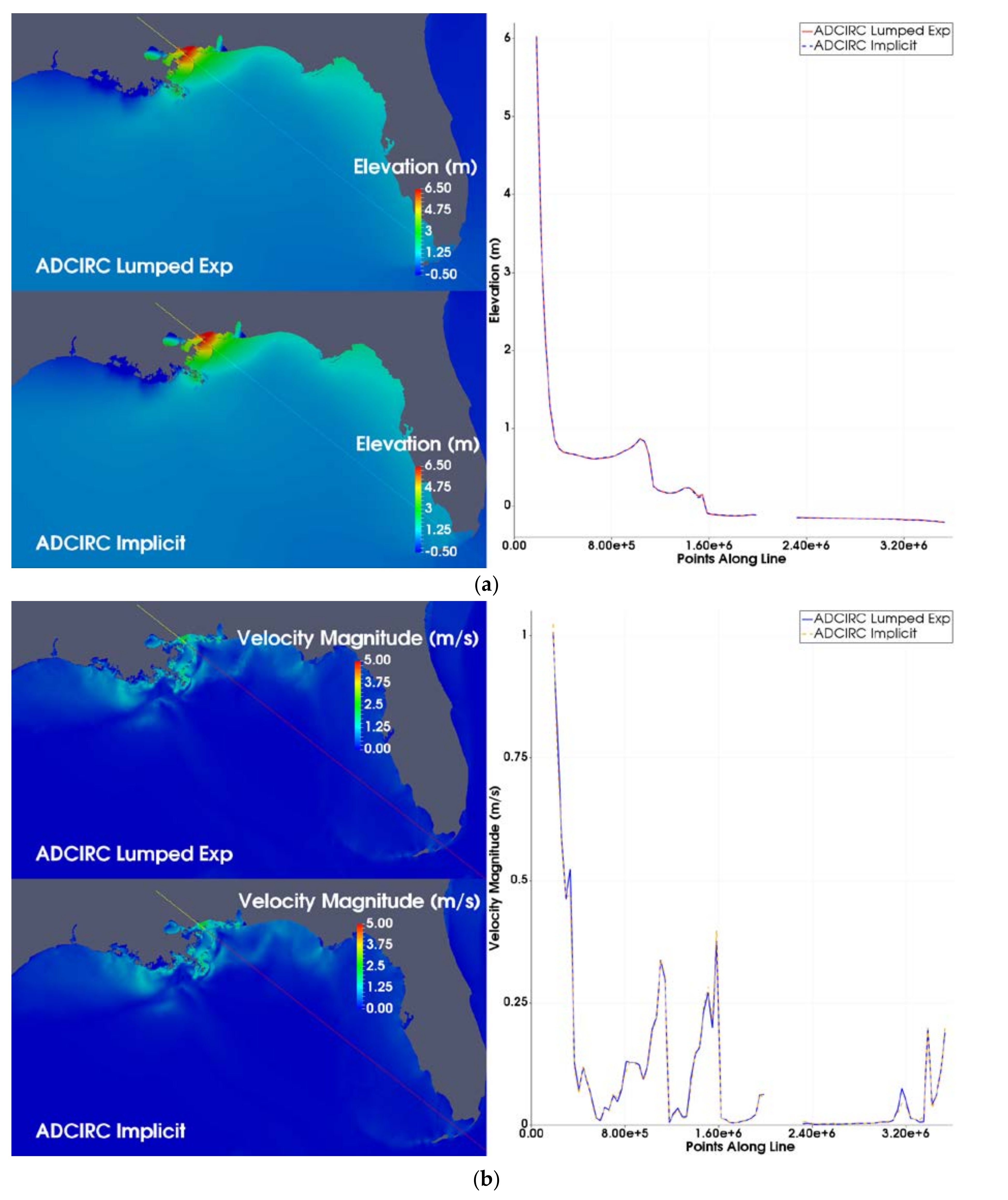
Maximum water elevation and velocity color plots for the simulated storm surges are displayed in Figure 1. Line plots are shown along an arbitrary line that goes over the mainland near the hurricane’s landfall, the Gulf of Mexico, and islands located deep in the Atlantic Ocean. Comparisons of line plots between the lumped explicit (Case 1) and implicit (Case 5); and semi-implicit (Case 3) and implicit (Case 5) solvers are done on the right side of the color plots. Figure 1 confirms the overall accuracy and consistency among the results from different solvers with a few mismatches, even though their mathematical representations and solution techniques are significantly different.
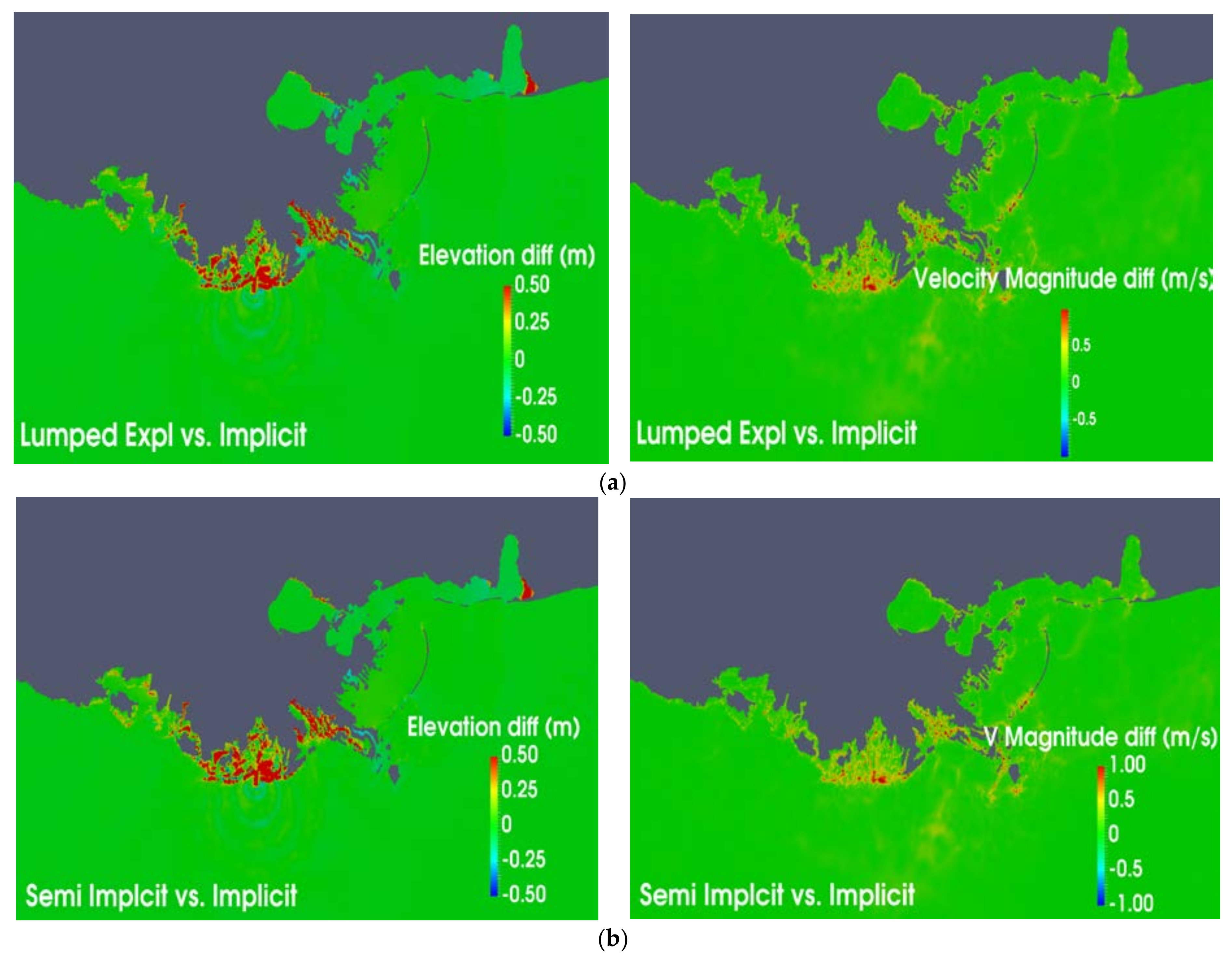
Figure 2 shows time snapshot differences of simulated water elevation and velocity magnitude at 10 AM on 29 August 2005 UTC from different solvers. It is evident that there are some differences in elevation and velocity results between the solvers near shorelines. Such differences are reported by other researchers [5,21], and these are attributed to ADCIRC wetting and drying convergence issues due to the lack of mesh refinement in the shallow water regions. Note that velocities are less impacted by the choice of solvers.
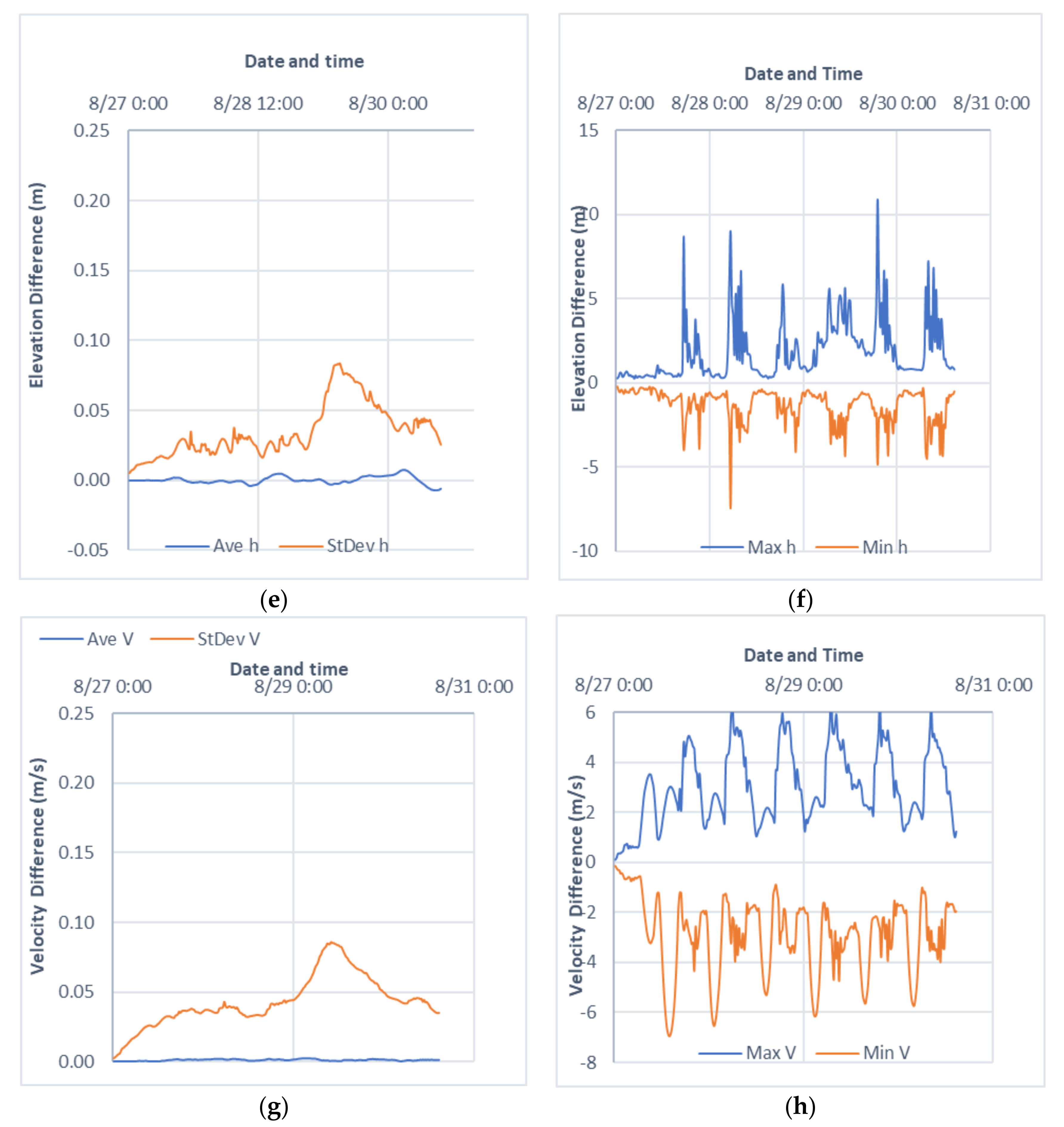
A time series of some statistical properties of the differences of water elevation and velocity simulated by different solvers are presented in Figure 3. The averages, standard deviations, maximums and minimums of those differences are calculated at all timesteps for the entire wet mesh, as follows:
- For each timestep, the differences of elevation and velocity are calculated for all wet nodes of the mesh by subtracting elevation and velocity of the second solver, say Case 5, from those of the first solver, say Case 1 (e.g., h_diff = h_Case1—h_Case5; V_diff = V_Case1—V_Case5).
- The average and standard deviation for the above differences of water elevation and velocity are calculated for each timestep.
- Maximums and minimums of the above differences between the results of the two solvers are obtained to identify the worst node-to-node differences for each timestep.
Figure 3 shows the time series average, standard deviation, minimum and maximum of water elevation and velocity differences of the implicit (Case 5) from those of the ADCIRC lumped explicit (Case 1) and semi-implicit (Case 3) solvers. When comparing the differences between Case 1 and Case 5, it is found that the mesh average and standard deviation of the water elevation and velocity differences are less than 0.07 m and 0.09 m/s, respectively. The maximum and minimum water elevation and velocity differences are ±10 m and ±7 m/s, respectively. When comparing Case 3 with Case 5, the average and standard deviations of water elevation and velocity differences are less than 0.08 m and 0.09 m/s, respectively. The maximum and minimum water elevation and velocity differences are ±10 m and ±7 m/s, respectively. It should be noted that the ADCIRC lumped explicit and semi-implicit formulations use timestep average values of barotropic pressure gradients, Coriolis effects, free surface stresses, and bottom friction terms [5], whereas the implemented implicit solver uses new timestep values for these terms. Therefore, the differences of maximum and minimum values between Case 1 and Case 5, and Case 3 and Case 5, are expected. Note that the ADCIRC lumped explicit and semi-implicit solvers had an average and standard deviation of water elevation and velocity differences less than 0.07 m and 0.05 m/s, respectively [5]. They had a maximum and minimum elevation and velocity differences of ±8 m and ±5 m/s, respectively [5].
4.3. Impact of Timestep
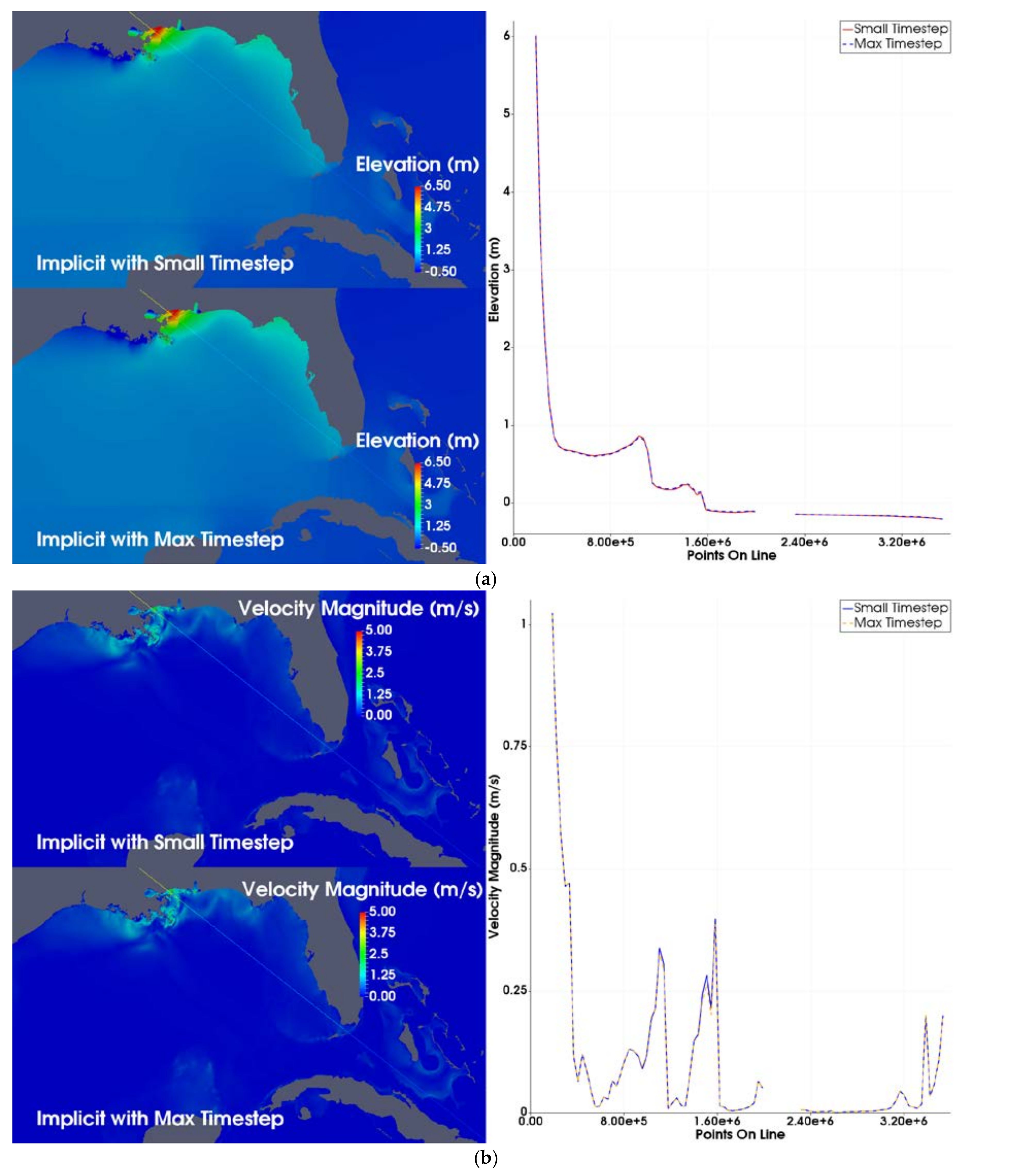
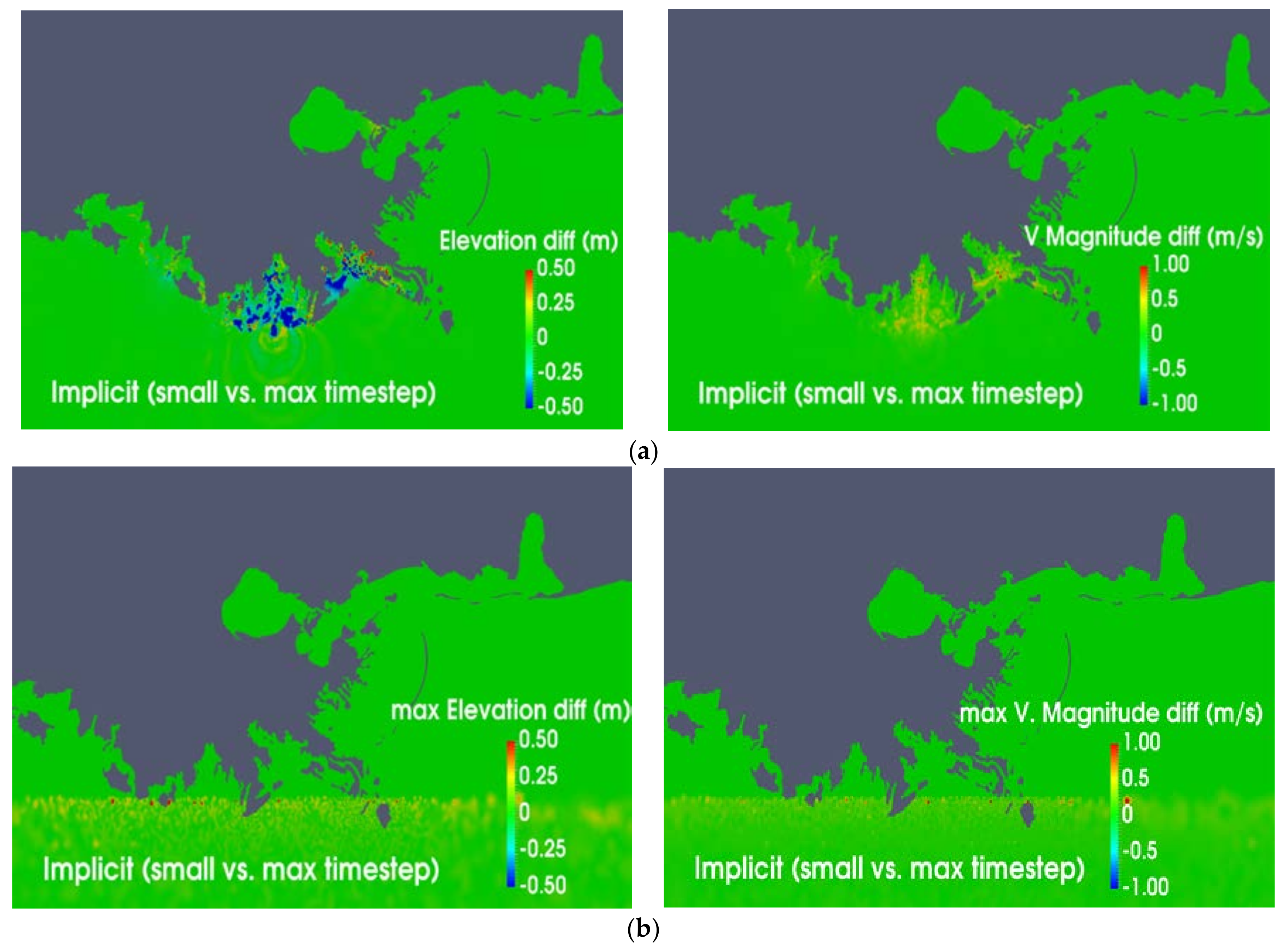
The impact of timestep on the implicit solver using small timestep (Case 5) and large timestep (Case 6) is investigated. Cases 5 and 6 use timestep size of 2 s and 120 s, respectively. The same arbitrary line, as in Figure 1, is used to create line plots for quantitative comparison between the two cases. Figure 4 presents the results of this experiment. Very few discrepancies are visible, which shows that even though Case 6 uses a significantly larger timestep, the results are still consistent with those of the smallest timestep used in Case 5. Moreover, a time snapshot and maximum and minimum elevation and velocity differences of both results are presented in Figure 5, which shows some discrepancies. A possible source of those mismatches is the evaluation of terms such as coriolis acceleration, barotropic pressure gradients, free surface stresses, and bottom friction in conservation equations where the transient components use previous time level values that might be greatly different near the wetting and drying regions at different times [5]. The velocity field seems to have less impact of timestep sizes than elevation. Recall that the implicit solver uses a nodal-based finite element technique for its elevation calculation, whereas an element center-based finite volume technique is used for its velocity calculation. Overall, it is a staggered mesh arrangement, which naturally suppresses any spurious oscillations. The result of Case 6 does not seem to be significantly different from that of Case 5, when putting the large difference of timesteps into perspective.
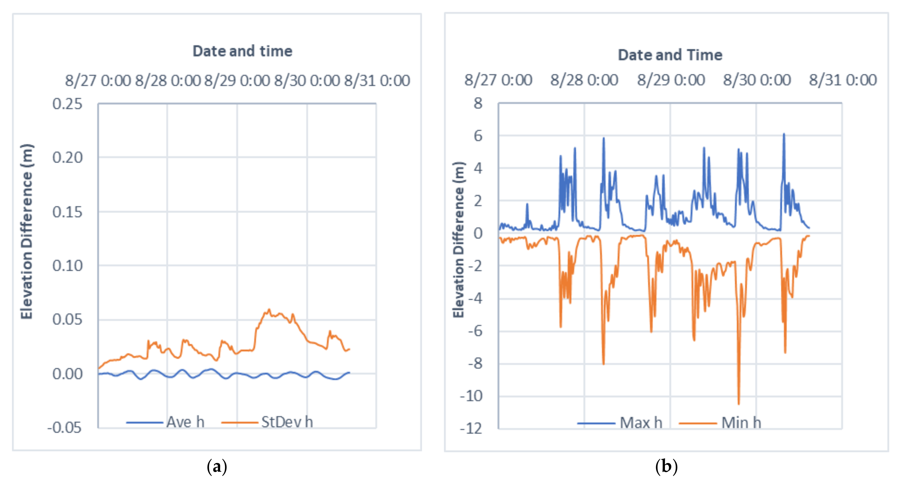
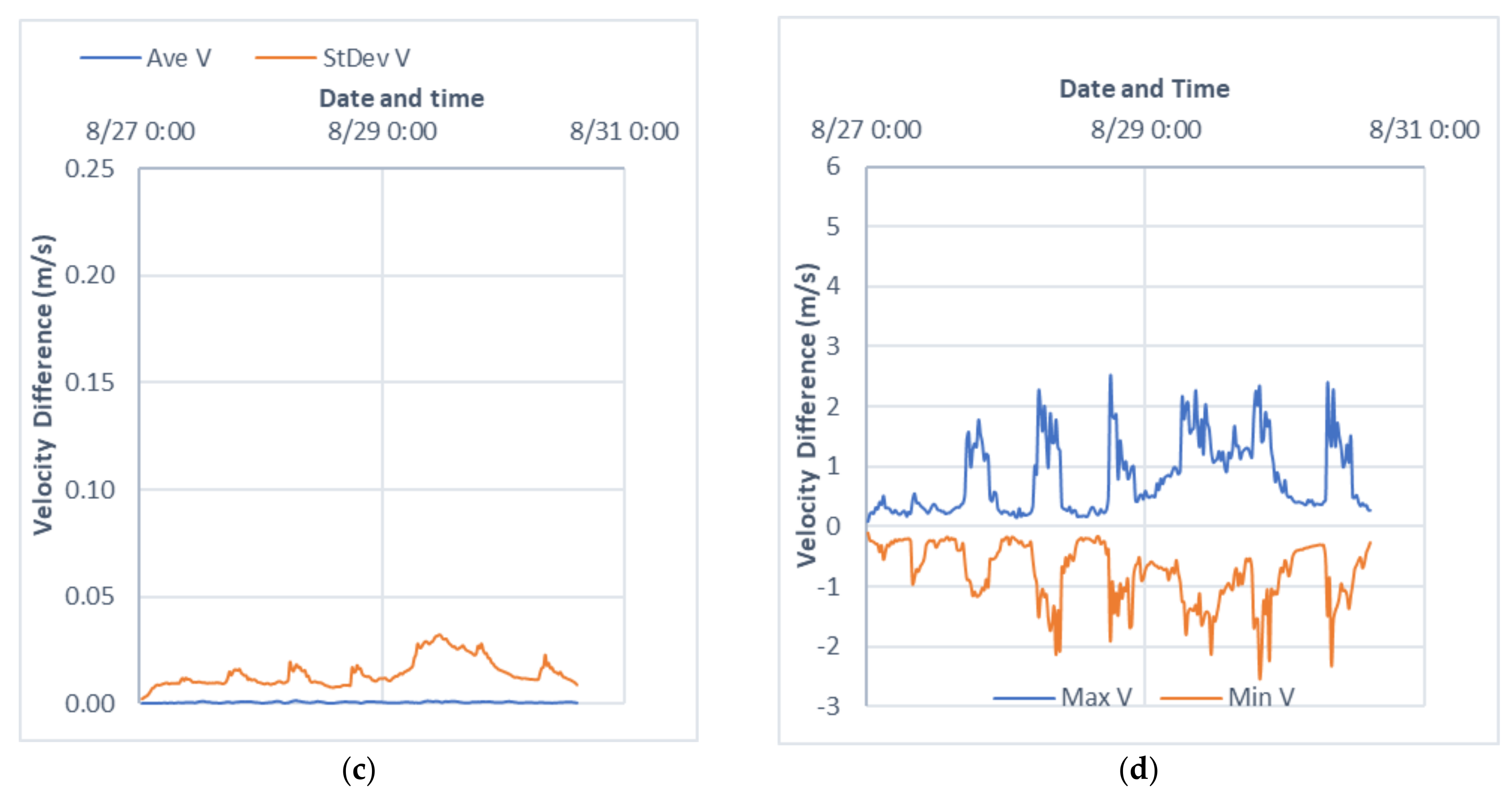
The time series average, standard deviation, minimum, and maximum of elevation and velocity differences for the wet mesh are calculated and plotted in Figure 6. The mesh average and standard deviation of water elevation and velocity differences are less than 0.06 m and 0.04 m/s, respectively. On the other hand, maximum and minimum water elevation differences are less than ±10 m, and maximum and minimum velocity differences are less than ±2.5 m/s.
4.4. Buoys Time Series Comparison
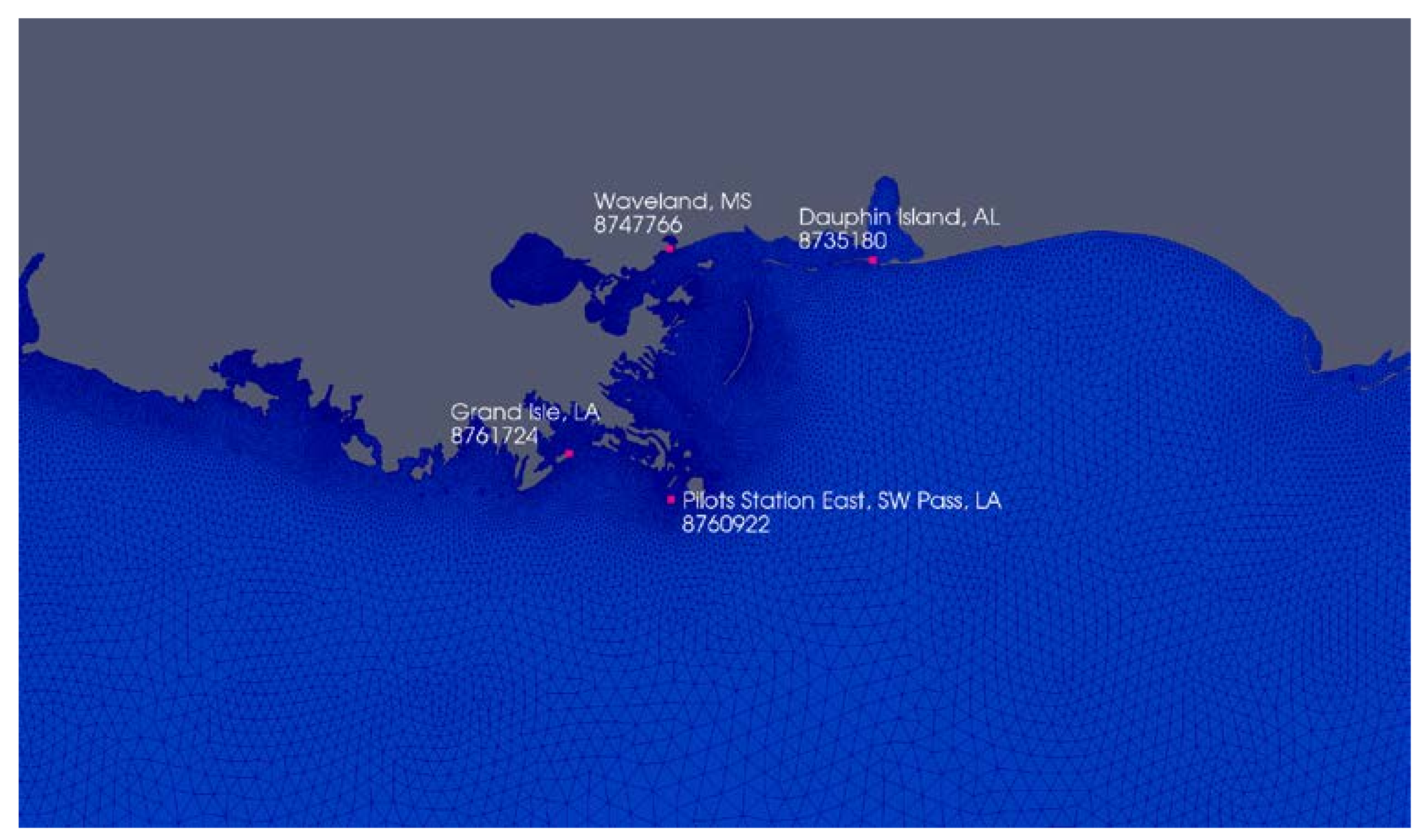
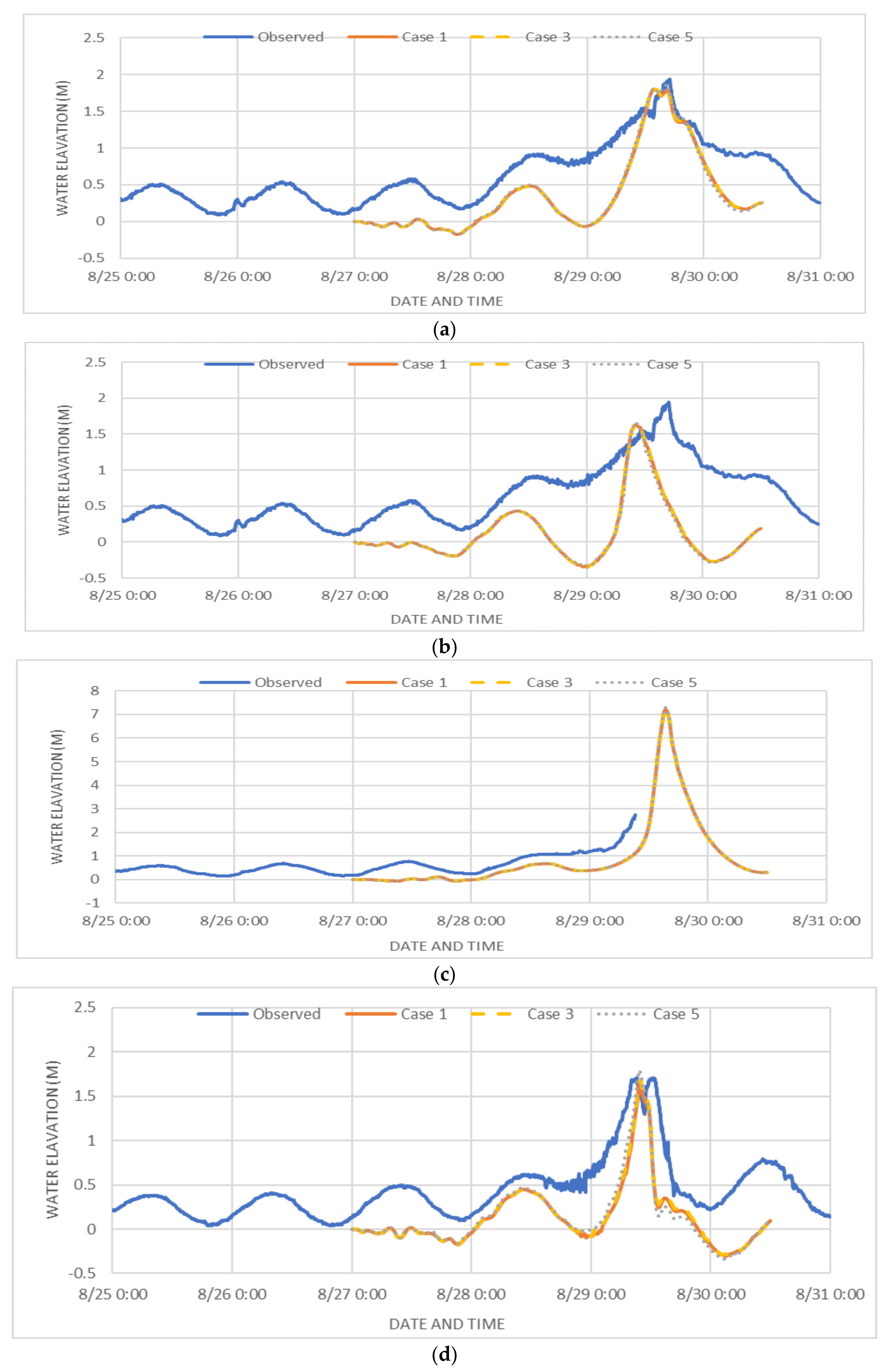
The time series data, collected during Hurricane Katrina using buoys and archived by NOAA [16], are used and compared with simulated results produced by Case 1, Case 3, and Case 5. There are four buoys for which time series data are available and whose locations fall within the computational domain used in the present study, as illustrated in Figure 7. The comparison between the simulated results and collected data is presented in Figure 8. It is obvious that implicit (Case 5) simulated results match reasonably well with the simulated results of the other two solvers (Cases 1 and 3). It is worth mentioning that mismatches between the observed and simulated results are reported by other researchers as well [22]. The surface waves are neglected in these simulations, which has most likely contributed to under prediction of water elevation. It is worth mentioning that implicit solver integration with the surface wave model (SWAN) is not implemented or experimented yet. Note that the Waveland MS buoy (ID 8747766) experienced a failure starting at 9 a.m. on 29 August 2005 UTC, which is why there is no data after that time.
4.5. High Water Mark Comparison
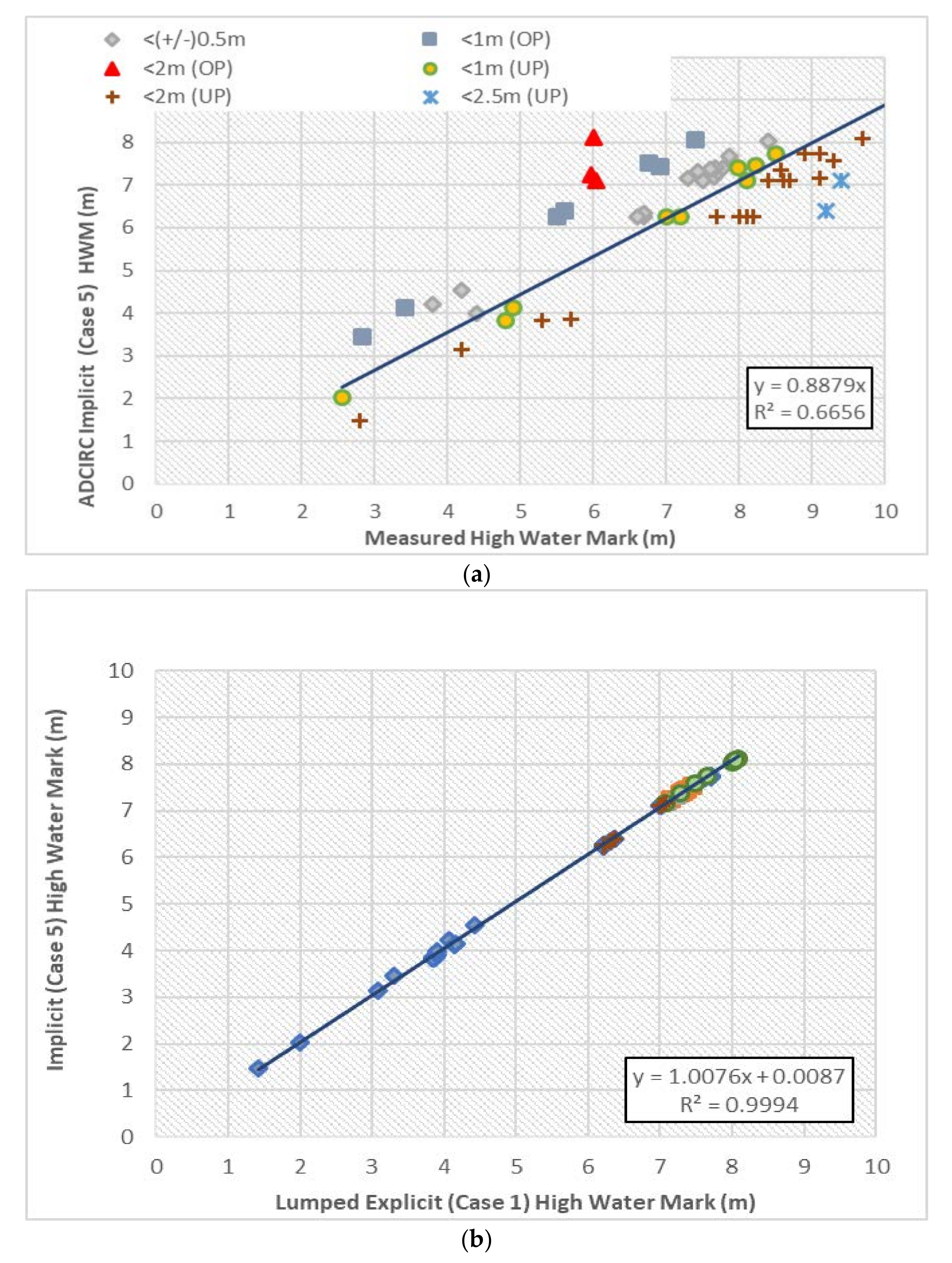
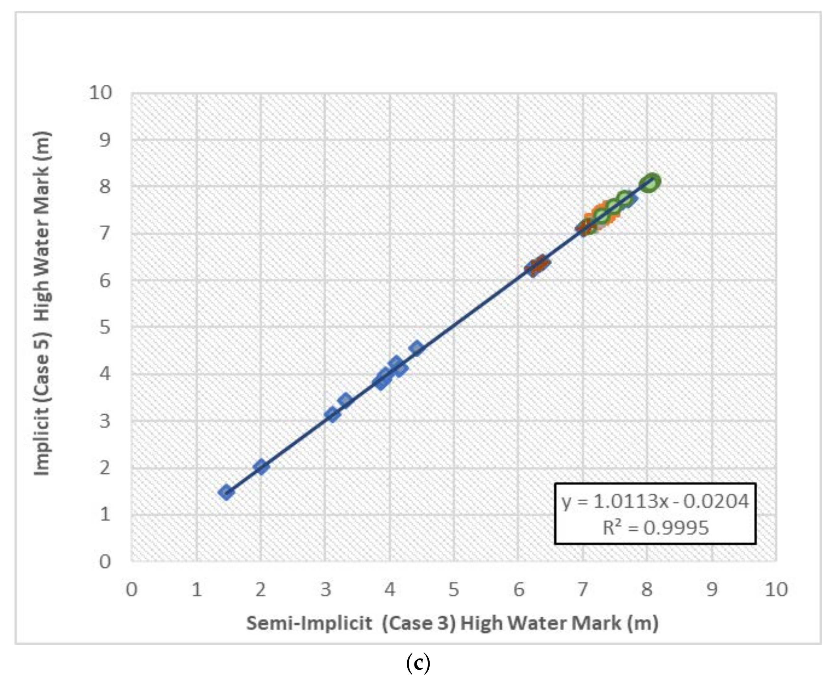
The Federal Emergency Management Agency (FEMA) measured high-water marks (HWM) after Hurricane Katrina had passed [23,24,25]. The HWM data is compared with results simulated by the implicit solver (Case 5). In addition to that, comparisons between implicit (Case 5) and lumped explicit (Case 1), implicit (Case 5) and semi-implicit (Case 3) are performed. In the present mesh, a total of 59 HWM stations are consistently wet in all simulations done using three solvers used here. The results are presented in Figure 9. It is worth mentioning that there are a number of well-known deficiencies with storm surge model setups such as: limitation of the PBL model in producing accurate wind fields, absence of near shore waves, inadequate bathymetry-specific bottom friction tuning, decreased wind drag over water, wrongful measurement of local water depth and land elevation, etc. [5]. When the result of the implicit solver is compared against the observed high water mark data in Figure 8a, a linear fit with a coefficient of determination (R2) value of 0.666 is obtained, similar to the ones reported in [5]. This value of R2 is considered very good in perspective since even a sophisticated mesh and model setup for Hurricane Ike, which had the maximum water elevation of 5 m, the best fit for ADCIRC produced R2 value of 0.716 [26]. Most importantly, the implicit solver (Case 5) gives almost identical results to the ones produced by the lumped explicit (Case 1) and semi-implicit (Case 3) solvers, as shown in Figure 9b,c.
4.6. Execution Time
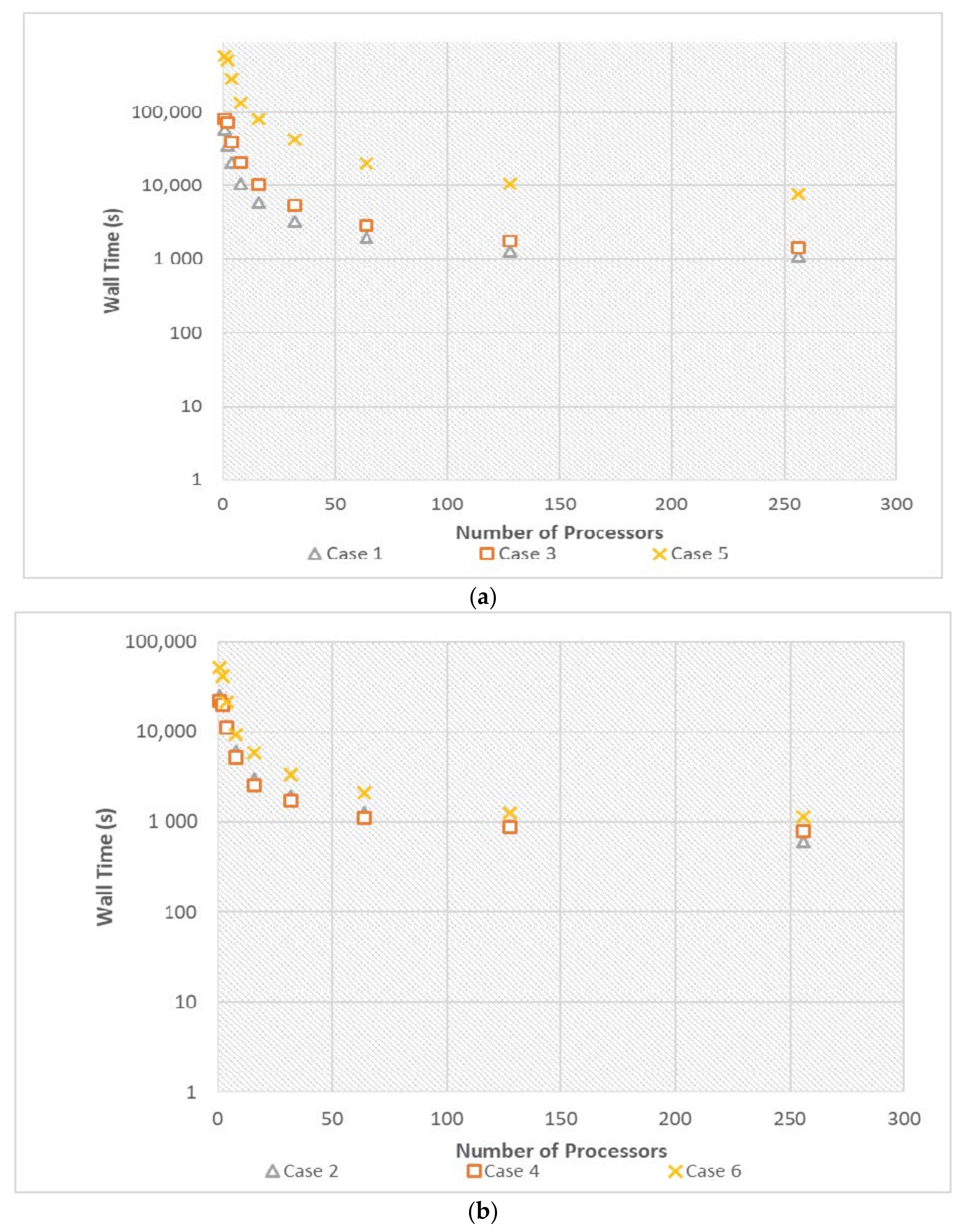
Some experiments are conducted to study the execution times of the implicit solver and compare the results with those of the other ADCIRC solvers. The number of processors used in these experiments ranged from 1 to 256. The experiments are divided into two parts. The smallest timestep (2 s, Cases 1, 3, and 5) for all solvers is used to run the first part of experiments; the findings are presented in Table 3. The largest timesteps for all solvers (Cases 2, 4, and 6) are used to run the second part of experiments. Table 4 presents the findings of all these extreme cases. Figure 10 shows plots of execution time comparison. Regarding execution time, it is evident that the lumped explicit, and semi-implicit solvers surpass the implicit solver in all experiments. When comparing with the extreme cases presented by Akbar et al. [5], the ADCIRC implicit solver (Case 6, execution time 1142 s) is slightly faster than the fully implicit solver of CaMEL (execution time 1205 s) presented in [5]. The gained speed can be partially attributed to the efficient parallel environment of ADCIRC. Note that the number of nonlinear iterations impacts the execution time performance of the implicit solver, which uses an iterative solution technique. It should be mentioned that repeated experiments show a slight variability of execution times due to the load conditions of servers.
5. Conclusions
Although hurricanes have many aspects that need to be studied, this paper focuses on the implementation of an implicit solver in the ADCIRC storm surge model. The CaMEL implicit solver solves the shallow water equations using hybrid finite element and finite volume techniques. Enhancing numerical stability, providing an option of using large timesteps, taking advantage of efficient parallel framework of ADCIRC, and reducing the complexity of mathematical formulation of ADCIRC are among the main objectives of this implicit solver implementation. In all experiments, Hurricane Katrina hindcast is done using the same mesh and similar input variables in different solvers to guarantee the validity of these experiments. Comparisons of results of the implicit solver with those of the lumped explicit and semi-implicit solvers are performed. Solver stability, accuracy and consistency of water elevation and velocity results, impact of timesteps, comparison of simulated results with observed data of buoys and HWMs, and execution times are studied. In general, results of the implicit solver are very well comparable with those of other solvers. The implicit solver shows great stability even when using large timesteps. The lumped explicit solver outperforms both semi-implicit and implicit ones regarding speed and execution times. The solver execution times are comparable when extreme timesteps are used, although the explicit solver still outperforms the other two. It should be noted that the current implementation of the implicit solver in ADCIRC is done on an ad hoc basis to study the feasibility, and no optimization is done at this point.
Author Contributions
A.A. performed the research in close collaboration with M.A. A.A. prepared the first draft of the manuscript. M.A. performed the technical review and modifications.
Acknowledgments
The authors would like to thank Renaissance Computing Institute (RENCI) for providing access to High Performance Computing (HPC) environment. Special thanks dedicated to Najran University, Saudi Arabia, for their scholarship program.
Conflicts of Interest
The authors declare no conflict of interest.
References
- Hurricanes: A Perfect Storm of Chance and Climate Change. Available online: http://www.bbc.com/news/science-environment-41347527 (accessed on 13 March 2018).
- Luettich, R.A.; Westerink, J.J. Formulation and Numerical Implementation of the 2D/3D ADCIRC Finite Element Model Version 44.XX. 8 December 2004. Available online: http://www.unc.edu/ims/adcirc-/adcirc_theory_2004_12_08.pdf (accessed on 5 March 2018).
- Akbar, M.K.; Aliabadi, S. Hybrid numerical methods to solve shallow water equations for hurricane induced storm surge modeling. Environ. Model. Softw. 2013, 46, 118–128. [Google Scholar] [CrossRef]
- Luettich, R.A.; Westerink, J.J.; Scheffner, N.W. ADCIRC: An Advanced Three-Dimensional Circulation Model for Shelves, Coasts and Estuaries. Report 1: Theory and Methodology of ADCIRC-2DDI and ADCIRC-3DL; Technical Report DRP-92-6; Department of the Army, USACE: Washington, DC, USA, 1991. [Google Scholar]
- Akbar, M.K.; Luettich, R.A.; Fleming, J.G.; Aliabadi, S.K. CaMEL and ADCIRC Storm Surge Models—A Comparative Study. J. Mar. Sci. Eng. 2017, 5, 35. [Google Scholar] [CrossRef]
- Dresback, K.M.; Kolar, R.L.; Dietrich, J.C. Impact of the form of the momentum equation on shallow water models based on the generalized wave continuity equation. Dev. Water Sci. 2002, 47, 1573–1580. [Google Scholar]
- Aliabadi, S.; Akbar, M.; Patel, R. Hybrid finite element/volume method for shallow water equations. Int. J. Numer. Methods Eng. 2010, 83, 1719–1738. [Google Scholar] [CrossRef]
- Westerink, J.J.; Luettich, R.A.; Blain, C.A.; Scheffner, N.W. An Advanced Three-Dimensional Circulation Model for Shelves, Coasts and Estuaries. Report 2: Users’ Manual for ADCIRC-2DDI; Department of the Army, USACE: Washington, DC, USA, 1992. [Google Scholar]
- Bunya, S.; Dietrich, J.C.; Westerink, J.J.; Ebersole, B.A.; Smith, J.M.; Atkinson, J.H.; Jensen, R.; Resio, D.T.; Luettich, R.A.; Dawson, C.; et al. A High-Resolution Coupled Riverine Flow, Tide, Wind, Wind Wave, and Storm Surge Model for Southern Louisiana and Mississippi. Part I: Model Development and Validation. Mon. Weather Rev. 2000, 138, 345–377. [Google Scholar] [CrossRef]
- Kolar, R.L.; Gray, W.G.; Westerink, J.J.; Luettich, R.A., Jr. Shallow water modeling in spherical coordinates: Equation formulation, numerical implementation, and application. J. Hydraul. Res. 1994, 32, 3–24. [Google Scholar] [CrossRef]
- Blain, C.A.; Rogers, W.E. Coastal Tide Prediction Using the ADCIRC-2DDI Hydrodynamic Finite Element Model: Model Validation and Sensitivity Analyses in the Southern North Sea/English Channel; Technical Report-NRL/FR/7322-98-9682; Naval Research Lab Stennis Space Center MS Coastal and Semi-Enclosed Seas Section: Washington, DC, USA, 1998. [Google Scholar]
- Tu, S.; Aliabadi, S.; Patel, R.; Watts, M. An Implementation of the Spalart-Allmaras DES Model in an Implicit Unstructured Hybrid Finite Volume/Element Solver for Incompressible Turbulent Flow. Int. J. Numer. Methods Fluids 2009, 59, 1051–1062. [Google Scholar] [CrossRef]
- Tu, S.; Aliabadi, S. Development of a Hybrid Finite Volume/Element Solver for Incompressible Flows. Int. J. Numer. Methods Fluids 2007, 55, 177–203. [Google Scholar] [CrossRef]
- Timmermans, L.J.P.; Minev, P.D.; Van De Vosse, F.N. An approximate projection scheme for incompressible flow using spectral elements. Int. J. Numer. Methods Fluids 1996, 22, 673–688. [Google Scholar] [CrossRef]
- Aliabadi, S. Parallel Finite Element Computations in Aerospace Applications. Ph.D. Thesis, University of Minnesota, Minneapolis, MN, USA, 1994. [Google Scholar]
- NOAA. National Oceanic and Atmospheric Administration. Available online: http://www.noaa.gov/ (accessed on 5 March 2018).[Green Version]
- Mukai, A.Y.; Westerink, J.J.; Luettich, R.A., Jr. Guidelines for Using the Eastcoast 2001 Database of Tidal Constituents within the Western North Atlantic Ocean, Gulf of Mexico and Caribbean Sea, Coastal and Hydraulic Engineering Technical Note (IV-XX). 2002. Available online: http://www.unc.edu/ims/adcirc/publications/2002/2002_Mukai02.pdf (accessed on 5 March 2018).
- RENCI. Renaissance Computing Institute. Available online: http://renci.org/ (accessed on 4 February 2018).
- Predicting Hurricane Storm Surge and Waves Precisely. Available online: http://renci.org/wp-content/uploads/2014/08/2014_RENCI_Dell-CaseStudy.pdf (accessed on 2 February 2018).
- Alghamdi, A.; Akbar, M. Profiling and Evaluation of Implicit and Explicit Storm Surge Models. Int. J. Comput. Theory Eng. 2017, 9, 417–421. [Google Scholar] [CrossRef]
- Tanaka, S.; Bunya, S.; Westerink, J.J.; Dawson, C.; Luettich, R.A. Scalability of an Unstructured Grid Continuous Galerkin Based Hurricane Storm Surge Model. J. Sci. Comput. 2011, 46, 329–358. [Google Scholar] [CrossRef]
- Blain, C.A.; Massey, T.C.; Dykes, J.D.; Posey, P.G.; Naval Research Lab Stennis Space Center MS Oceanography Div. Advanced Surge and Inundation Modeling: A Case Study from Hurricane Katrina; Stennis Space Center: Hancock County, MS, USA, 2007. [Google Scholar]
- FEMA. High Water Mark Collection for Hurricane Katrina in Louisiana; FEMA-1603-DR-LA, Task Orders 412 and 419; Federal Emergency Management Agency: Denton, TX, USA, 2006.
- FEMA. Final Coastal and Riverine High Water Mark Collection for Hurricane Katrina in Mississippi; FEMA-1604-DR-MS, Task Orders 413 and 420; Federal Emergency Management Agency: Atlanta, GA, USA, 2006.
- FEMA. High Water Mark Collection for Hurricane Katrina in Alabama; FEMA-1605-DR-AL, Task Orders 414 and 421; Federal Emergency Management Agency: Atlanta, GA, USA, 2006.
- Kerr, P.C.; Donahue, A.S.; Westerink, J.J.; Luettich, R.A.; Zheng, L.Y.; Weisberg, R.H.; Huang, Y.; Wang, H.V.; Teng, Y.; Forrest, D.R.; et al. US IOOS coastal and ocean modeling testbed: Inter-model evaluation of tides, waves, and hurricane surge in the Gulf of Mexico. J. Geophys. Res. Oceans 2013, 118, 5129–5172. [Google Scholar] [CrossRef]
Figure 1.
Maximum elevation and velocity comparison study: (a) Elevation of Lumped Explicit (Case 1) vs. Implicit (Case 5); (b) velocity magnitude of Lumped Explicit (Case 1) vs. Implicit (Case 5); (c) elevation of Semi-Implicit (Case 3) vs. Implicit (Case 5); (d) velocity magnitude of Semi-Implicit (Case 3) vs. Implicit (Case 5).


Figure 2.
Time snapshot differences of simulated water elevation and velocity magnitude at 10 a.m. on 29 August 2005 UTC between: (a) Lumped Explicit (Case 1) vs. Implicit (Case 5); (b) Semi-Implicit (Case 3) vs. Implicit (Case 5).
Figure 2.
Time snapshot differences of simulated water elevation and velocity magnitude at 10 a.m. on 29 August 2005 UTC between: (a) Lumped Explicit (Case 1) vs. Implicit (Case 5); (b) Semi-Implicit (Case 3) vs. Implicit (Case 5).

Figure 3.
Time series average (‘Ave’), standard deviation (‘StDev’), minimum (‘Min’) and maximum (‘Max’) of water elevation and velocity differences between: (a–d) Lumped Explicit (Case 1) vs. Implicit (Case 5), and (e–h) Semi-Implicit (Case 3) vs. Implicit (Case 5).
Figure 3.
Time series average (‘Ave’), standard deviation (‘StDev’), minimum (‘Min’) and maximum (‘Max’) of water elevation and velocity differences between: (a–d) Lumped Explicit (Case 1) vs. Implicit (Case 5), and (e–h) Semi-Implicit (Case 3) vs. Implicit (Case 5).
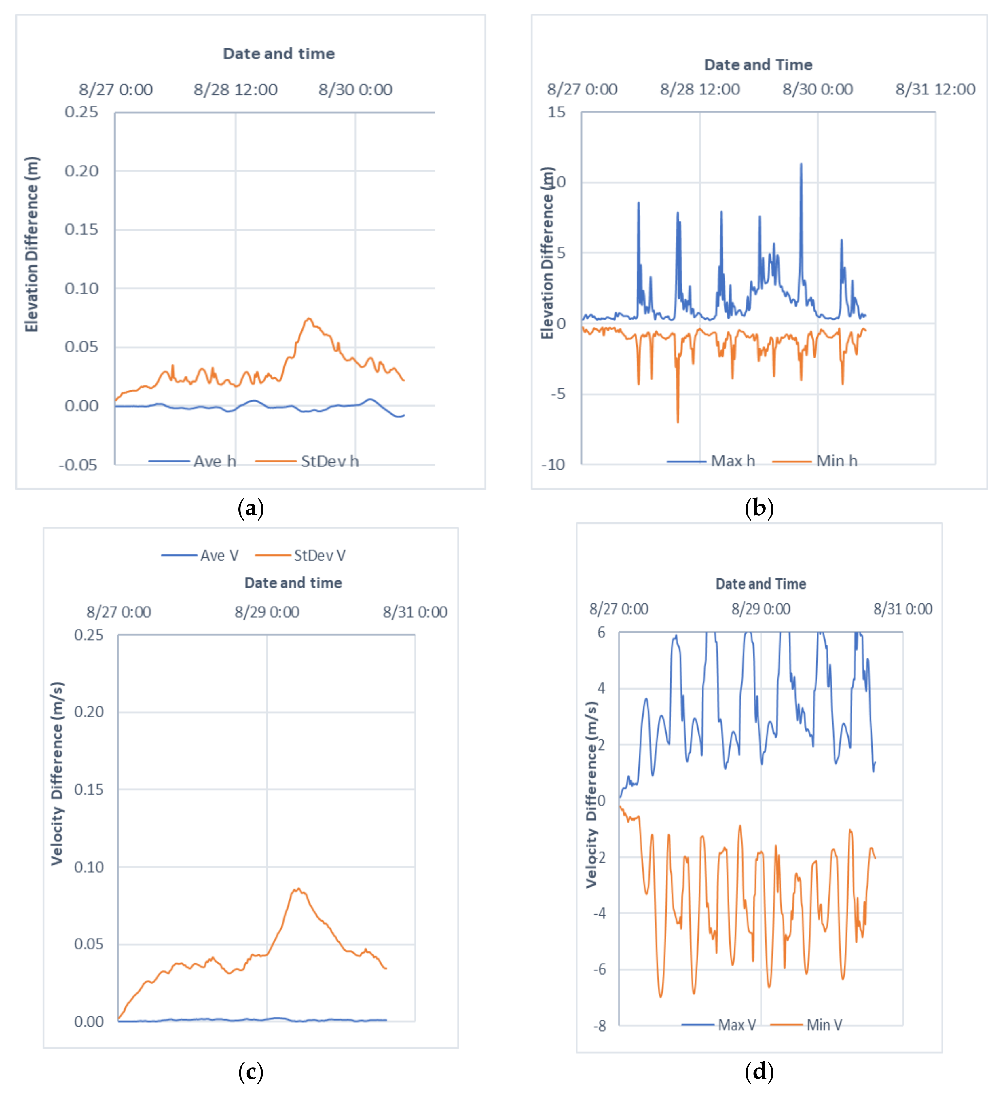

Figure 4.
Maximum elevation and velocity comparison for timestep size study: (a) Elevation of Implicit (Case 5) vs. Implicit (Case 6); (b) velocity magnitude of Implicit (Case 5) vs. Implicit (Case 6).
Figure 4.
Maximum elevation and velocity comparison for timestep size study: (a) Elevation of Implicit (Case 5) vs. Implicit (Case 6); (b) velocity magnitude of Implicit (Case 5) vs. Implicit (Case 6).

Figure 5.
Implicit solver (Case 5) vs. Implicit solver (Case 6): (a) Time snapshot differences of water elevation and velocity magnitude at 10 a.m. on 29 August 2005 UTC. (b) Maximum elevation and velocity differences.
Figure 5.
Implicit solver (Case 5) vs. Implicit solver (Case 6): (a) Time snapshot differences of water elevation and velocity magnitude at 10 a.m. on 29 August 2005 UTC. (b) Maximum elevation and velocity differences.

Figure 6.
Impact of timesteps on Implicit solver between small (Case 5) and large (Case 6) steps: (a) Elevation time series average and standard deviation; (b) minimum and maximum of water elevation; (c) velocity time series average and standard deviation; (d) minimum and maximum of water velocity.
Figure 6.
Impact of timesteps on Implicit solver between small (Case 5) and large (Case 6) steps: (a) Elevation time series average and standard deviation; (b) minimum and maximum of water elevation; (c) velocity time series average and standard deviation; (d) minimum and maximum of water velocity.


Figure 7.
The region of interest with NOAA tide and current stations during Hurricane Katrina.

Figure 8.
Observed time series data vs. modeled time series results of Hurricane Katrina storm surge: (a) Station ID 8735180 Dauphin Island AL; (b) Station ID 8735180 Pilots Station East SW Pass LA; (c) Station ID 8747766 Waveland MS; and (d) Station ID 8761724 Grand Isle.
Figure 8.
Observed time series data vs. modeled time series results of Hurricane Katrina storm surge: (a) Station ID 8735180 Dauphin Island AL; (b) Station ID 8735180 Pilots Station East SW Pass LA; (c) Station ID 8747766 Waveland MS; and (d) Station ID 8761724 Grand Isle.

Figure 9.
Hurricane Katrina HWM comparisons: (a) Observed data vs. Implicit Solver (Case 5); (b) Lumped Explicit Solver (Case 1) vs. Implicit Solver (Case 5); (c) Semi-Implicit Solver (Case 3) vs. Implicit Solver (Case 5).
Figure 9.
Hurricane Katrina HWM comparisons: (a) Observed data vs. Implicit Solver (Case 5); (b) Lumped Explicit Solver (Case 1) vs. Implicit Solver (Case 5); (c) Semi-Implicit Solver (Case 3) vs. Implicit Solver (Case 5).


Figure 10.
Execution times comparison between Lumped Explicit, Semi-Implicit, and Implicit solvers using Hurricane Katrina hindcast: (a) Execution time using the same timestep (Cases 1, 3, and 5) for all solvers (see Table 3); (b) execution time using maximum timesteps (Cases 2, 4, and 6) to each solver (see Table 4).


Table 1.
Stability Study of ADCIRC Solvers.
| Timestep (s) | Lumped Explicit | Semi-Implicit | Implicit | ||||
|---|---|---|---|---|---|---|---|
| Comment | Walltime (s) | Comment | Walltime (s) | Comment | Walltime (s) | Nonlinear Iterations | |
| 2 | Success | 1283 | Success | 1771 | Success | 10,466 | 2 |
| 4 | Success | 902 | Success | 1130 | Success | 5712 | 2 |
| 8 | Fail | N/A | Success | 866 | Success | 3497 | 2 |
| 12 | Fail | N/A | Success | 2685 | 2 | ||
| 40 | Success | 1368 | 2 | ||||
| 100 | Success | 1213 | 3 | ||||
| 120 | Success | 1272 | 4 | ||||
| 150 | Fail | N/A | 6 | ||||
Table 2.
Experimental Run Cases.
| Case # | Solver | Timestep (s) |
|---|---|---|
| 1 | Lumped Explicit | 2 |
| 2 | Lumped Explicit | 4 |
| 3 | Semi-Implicit | 2 |
| 4 | Semi-Implicit | 8 |
| 5 | Implicit | 2 |
| 6 | Implicit | 120 |
Table 3.
ADCIRC Solvers Execution Times in Seconds (timestep 2 s).
| No. of CPUs | ADCIRC Lumped Explicit Case 1 | ADCIRC Semi-Implicit Case 3 | ADCIRC Implicit Case 5 |
|---|---|---|---|
| 1 | 58,591 | 79,686 | 572,863 |
| 2 | 35,390 | 72,672 | 500,688 |
| 4 | 20,571 | 39,423 | 276,973 |
| 8 | 10,662 | 20,487 | 131,750 |
| 16 | 5837 | 10,149 | 80,415 |
| 32 | 3224 | 5438 | 42,342 |
| 64 | 1951 | 2855 | 19,901 |
| 128 | 1283 | 1771 | 10,466 |
| 256 | 1097 | 1440 | 7657 |
Table 4.
ADCIRC Solvers Execution Times in Seconds (extreme cases).
| No. of CPUs | ADCIRC Lumped Explicit Case 2 | ADCIRC Semi-Implicit Case 4 | ADCIRC Implicit Case 6 |
|---|---|---|---|
| 1 | 25,062 | 21,970 | 52,528 |
| 2 | 21,693 | 20,107 | 41,529 |
| 4 | 11,531 | 11,083 | 21,747 |
| 8 | 6024 | 5267 | 9467 |
| 16 | 2958 | 2539 | 5942 |
| 32 | 1930 | 1750 | 3364 |
| 64 | 1259 | 1104 | 2128 |
| 128 | 902 | 866 | 1272 |
| 256 | 602 | 785 | 1142 |
© 2018 by the authors. Licensee MDPI, Basel, Switzerland. This article is an open access article distributed under the terms and conditions of the Creative Commons Attribution (CC BY) license (http://creativecommons.org/licenses/by/4.0/).
Share and Cite
MDPI and ACS Style
Alghamdi, A.; Akbar, M.K. Implementation of an Implicit Solver in ADCIRC Storm Surge Model. J. Mar. Sci. Eng. 2018, 6, 62. https://doi.org/10.3390/jmse6020062
AMA Style
Alghamdi A, Akbar MK. Implementation of an Implicit Solver in ADCIRC Storm Surge Model. Journal of Marine Science and Engineering. 2018; 6(2):62. https://doi.org/10.3390/jmse6020062
Chicago/Turabian StyleAlghamdi, Abdullah, and Muhammad K. Akbar. 2018. "Implementation of an Implicit Solver in ADCIRC Storm Surge Model" Journal of Marine Science and Engineering 6, no. 2: 62. https://doi.org/10.3390/jmse6020062
Note that from the first issue of 2016, this journal uses article numbers instead of page numbers. See further details here.