Optimal Transmission of Interface Vibration Wavelets—A Simulation of Seabed Seismic Responses

Abstract

Seismic interface waves generated by seabed impacts are believed to have biological importance. Previous work on the effects of ocean piling and dredging studied water motion adjacent to the seabed, using sediment measurements as reviewed in the literature. This new modelling work has idealised the sediment data to a simple model with few parameters, and has shown how this leads to filtration of the applied energy to propagate simple seismic vibration wavelets. These special wavelets remain compact with high peak levels of the associated water particle velocity as they ripple outward, and provide a means of assessing the worst-case environmental impact. The form of this wavelet morphs from a hump shape to a dip and back, via intermediate forms which are here described in mathematical terms based on the Ricker form. Whilst the model structure is idealised it is much closer to reality than the Rayleigh and Scholte half-space models, but with only two more parameters required. The resultant wavelet peaks are propagated with values given by the optimal limit case of cylindrical spreading (ignoring absorption) which results in a relatively widespread impact.

1. Introduction

The propagation of interface waves at the boundaries between different media has been the subject of extensive study [1,2,3,4]. Interface waves propagating across the seabed are relevant to applications such as geophysical surveying, sub-bottom profiling, and seabed feature detection [5], and for studies of the exposure of benthic fauna to seabed vibration caused by marine construction techniques such as pile driving [6,7,8,9]. Many examples of benthic fauna have poor sensitivity to sound pressure waves, but show a high sensitivity to low-frequency particle motion, as described by Popper, Hawkins, and Nedelec et al. [10,11,12,13]. The effects of being shaken by water particle velocity (a vector) rather than squeezed by sound pressure (a scalar) are now better understood, but are necessarily more complex.

A source of seabed interface waves which has been of particular interest in recent studies is that of marine pile driving, which is a favoured method of marine construction for bridge foundations, oil and gas platforms, and offshore wind farms [14]. A number of studies have reported measurements of the seabed motion using geophones [15], and of the sound pressure and/or particle motion in the region just above the seabed [16]. Interface waves generated by such impulsive sources can have interesting features, and detailed modelling of the motion of the seabed and water after such impacts has already been reported by Hazelwood and Macey [17], where the particle motion of the water adjacent to interface seismic waves (ground roll) has been shown to be elliptical and vigorous. The measurements on which this work was based came from trials of dredging by Robinson et al., 2011 [18] and of piling by Jansen et al., 2011 [19].

In this paper, a new half-space physical model for the propagation of seabed interface waves has been studied using finite element (FE) analysis and wavenumber integration. This sediment structure has properties which are graded with depth, wherein shear wave speeds increase linearly with depth after a step change at the interface. Such a seabed is shown to promote the propagation of a special seismic wavelet, which retains its form over long distances, with its peak amplitude closely following a cylindrical spreading rule when absorption is ignored. The energy is not dissipated and its propagation is thus optimal, retaining its structure and detectability.

This paper is structured as follows: First, the basic properties of a half-space model are described, followed by the properties of the new half-space model which is proposed for the simulation of saturated sediments. Then the approximations required for the FE model are described, with the forcing impulse function and the resulting wavelet, followed by a comparison with the results of computer modelling by the method of wavenumber integration. The results from the transient FE modelling are used to determine the mathematics which govern the wavelet, and its unusual propagation characteristics in this new physical model. Finally, there is a discussion and conclusion.

2. The Properties of Infinite Half-Space Models

Lord Rayleigh [1] described a physical model with a uniform solid below a horizontal interface. The solid and a vacuum above form two “half-spaces” extending to infinity. Interface waves supported by this model travel at a fixed speed determined by the speed of shear waves in the solid. With no variation of speed with frequency, communications are of good quality, as all waveforms are transmitted without distortion from a point source, giving a cylindrical spreading of the intensity. Scholte [2] showed that this also applied if the upper half-space was a uniform fluid.

Although a uniform solid is highly unrealistic, approximations can exist, particularly at high frequencies and small wavelengths, when only a thin layer is required to be uniform. Viktorov [3] described applications of Rayleigh waves for the detection of surface flaws. The evanescent nature of the waves, showing an exponential decay of amplitude with increasing distance from the interface, means that only surface properties are important. Real sedimentary properties change as the water is progressively excluded and the rigidity rises with depth, increasing the shear speed. Introduction of a speed profile has a dramatic effect on wave propagation, giving a variation of group speed with frequency content and consequent waveform distortion. It leads to frequency dispersion not seen in the original Rayleigh and Scholte models, as discussed by Achenbach [4].

Interface waves travelling across saturated sediments are slower than compression waves in the adjacent water, and they confine their energy to an evanescent form. In contrast, “leaky” waves travelling across stiff solid surfaces such as concrete, as modelled by Zhu et al. [20], radiate energy into the fluid and can be used to study surface flaws.

3. A New Half-Space Physical Model to Simulate Saturated Sediments

After using FE models with realistic sediment shear wave speeds as reviewed by Hamilton [21], a more idealised version has now been studied. We used a profile with an initial step rise at the interface, and a linear gradient, g_r, of the material shear speed thereafter. This contrasts with analyses of power-law profiles, including that of Chapman and Godin [22], where the shear waves, absent in the fluid, start with a wave speed of zero which increases with depth as a power law, favouring a special case of a half-power. When used with a constant density, this gives a linear increase in shear modulus, but still has a discontinuity of the gradient at the interface. In contrast, the model described here has a step change in shear speed at the seabed. We then find characteristic wavelets which propagate well, primarily influenced by sediment properties close to the seabed.

The Scholte half-space model requires both fluid and solid parameters to be specified. As with the Rayleigh model, the solid is specified by its uniform density, ρ_s, plus two independent mechanical properties, for example, the shear wave speed V_s and compressional wave speed V_p. Other options include the Young’s modulus E and Poisson ratio ν. The fluid half-space only needs its density ρ_w and the speed of water pressure waves, V_w, defined. The speed of the interface waves for the Rayleigh model is somewhat less than V_s, which, in turn, is less than V_p. For the special case when ν = 0.25 (a “Poisson solid”), the interface wave travels at ≈0.92 V_s. The same value has been chosen for this model, but only as a limit case at infinite depth. It is also reported for rocks such as granite, and was used by Zhu et al. [20] for concrete.

Whilst this graded seabed model remains idealised, it is very much more realistic than the uniform half-spaces of the Rayleigh and Scholte models. It requires one more parameter than did Scholte: the gradient g_r of V_s with depth, d. V_p also increases linearly, determined by the choice of ν = 0.25 at infinite depth. V_s and V_p now refer to the interface values which also control the values at depth d in the sediment:

$$V_s(d)=V_s+g_{r}d\hspace{0.17em}\hspace{0.17em}\hspace{0.17em}\hspace{0.17em}\hspace{0.17em}{V}_p(d)=V_p+\sqrt{3}{g}_{r}d.$$

4. The FE Model Simulates the Propagation of a Transient Ripple across the Interface

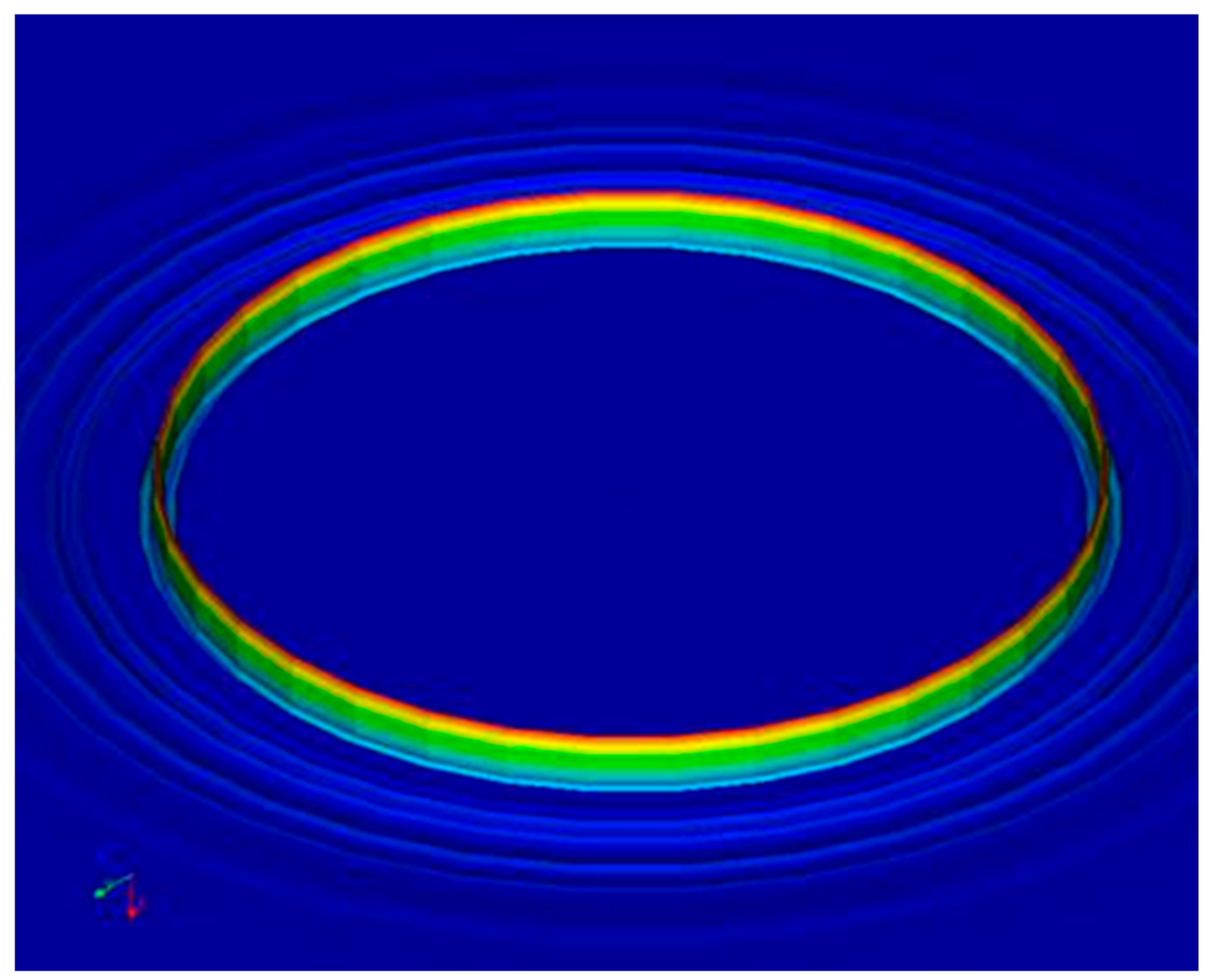
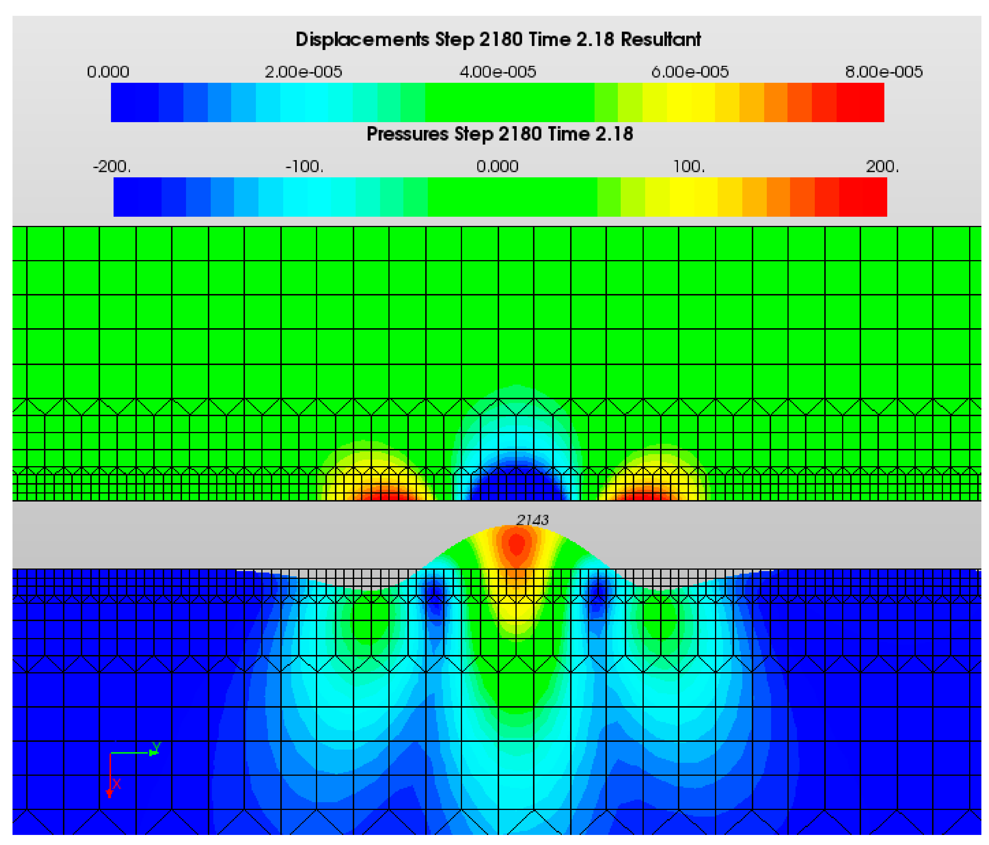
The three-dimensional view in Figure 1 can be compared with a two-dimensional (2D) cross section of FE displacement data in Figure 2, showing both the solid and the overlying water.

This idealised model is axisymmetric and was developed from a model of an underwater pile, providing a vertical force impulse at the axis of symmetry. Different techniques are used to calculate the sediment displacements and the pressures in the overlying water.

The finite elements shown in this 2D view use a refined solid mesh density near the seabed interface. The 16 m deep water layer is modelled by fluid elements, here shown separated from the solid by a 4 m gap to allow the exaggerated solid displacement to be seen. The solid elements (mostly not shown) extend to 128 m depth, where the base was usually held rigid. However, switching to a free base gave the same results, indicating that this deep sediment had little effect on the interface waves. This conclusion is supported by the small displacements predicted at depth, shown as deep blue in Figure 2. The linearly graded material properties used here have been substituted for those used in earlier FE models [17] derived from the review of published data by Hamilton [21].

The 16 m deep water layer can be deactivated where helpful. This changes the speed of propagation but otherwise has little effect. FE model parameters can be experimentally changed in a sequence of runs, such as the radial size of the elements. In Figure 2, the smallest elements are 0.5 m across, and successive calculations were made every 1 ms so that after 2180 steps the time since the start is 2.18 s. By then, the advanced ripples seen in Figure 1 have separated from the wavelet shown in Figure 2, which propagates stably as the greatest amplitude. The shear wave speed V_s, at the interface was 128 m/s. A small shear speed gradient g_r of 1 (m/s)/m, or 1 s⁻¹, was set for this model run. The compressive speed at the interface, V_p, was 1520 m/s. The solid had a uniform density of 2250 kg/m³. The water had a density of 1000 kg/m³ and wave speed of 1500 m/s.

5. Communications Would Be Distorted by Strong Filtration Imposed by the Sediment

This graded sediment physical model does not transmit signals with the high fidelity seen for the Rayleigh and Scholte models, with their uniform solid material properties, but shows a strong resonant filtration of the input energy. High-fidelity communication in air and water relies upon the wave speed being invariant with frequency to avoid distortion. When a pulse is applied to the graded solid model a characteristic waveform is seen, sometimes dominated by a “Ricker” mathematical form. Yanghua Wang [23] describes some features of this function which is widely used in seismology. Its use here for the FE driving force pulse simplifies the resultant wavelets. The consequent wavelet stability gives good correlation between results at different distances and times, increasing the precision of measurement of their speed.

The wavelet speed or group speed has been found to vary slightly with the driving pulse widths, but a succession of different width wavelets can still remain separated when transmitted over distances which are long compared with their width. This could allow a form of high-fidelity communication of a specialised nature for the deep-sea creatures discussed by Klages et al. [24]. This might complement the ability of benthic creatures to resolve the direction of wavelet propagation using their retrograde particle motion as predicted in the earlier paper [17].

6. The Structure of the Wavelet as a Combination of Hermite Polynomials

The structure of the wavelet is determined primarily by the solid material properties, principally the shear wave speed. The 16 m deep overlying water as seen in Figure 2 has been deactivated for some simpler “dry” runs which provided enlightenment with less FE computation. Whilst dry runs were useful, full wet runs were used to study the effect of the drive pulse width as the presence of water changes the wavelet speed.

The Ricker mathematical function (R_k), also described as a “Mexican Hat” [25], is used here to describe amplitude versus time t. Constants K, peak time t₀, and zero-to-zero width τ, can be adjusted to fit data from the FE analysis.

$$R_k(T)=K{e}^{\frac{-T^2}{2}}(1-T^2) \mathrm{where} T=\frac{2(t-t_0)}{\tau }$$

(1)

This function is the second derivative of a Gaussian probability (“bell”) curve, which provides the exponential kernel within Equation (1), with a peak amplitude K at T = 0. It diminishes to zero at infinity, but never crosses the axis to become negative. This form is convenient for differentiation, and repeated differentiation creates a series of functions. These form the Hermite polynomial sequence described by Hochstrasser [26], which when multiplied by this kernel creates wavelet shapes with increasing numbers of zero crossings. Each polynomial in the sequence He (n) of order n creates a wavelet with n zero crossings. They alternately give symmetric, even-order shapes such as the Ricker function (n = 2) and the Gaussian normal distribution (n = 0), and antisymmetric, odd-order shapes with an odd number of zero crossings, always including one at T = 0.

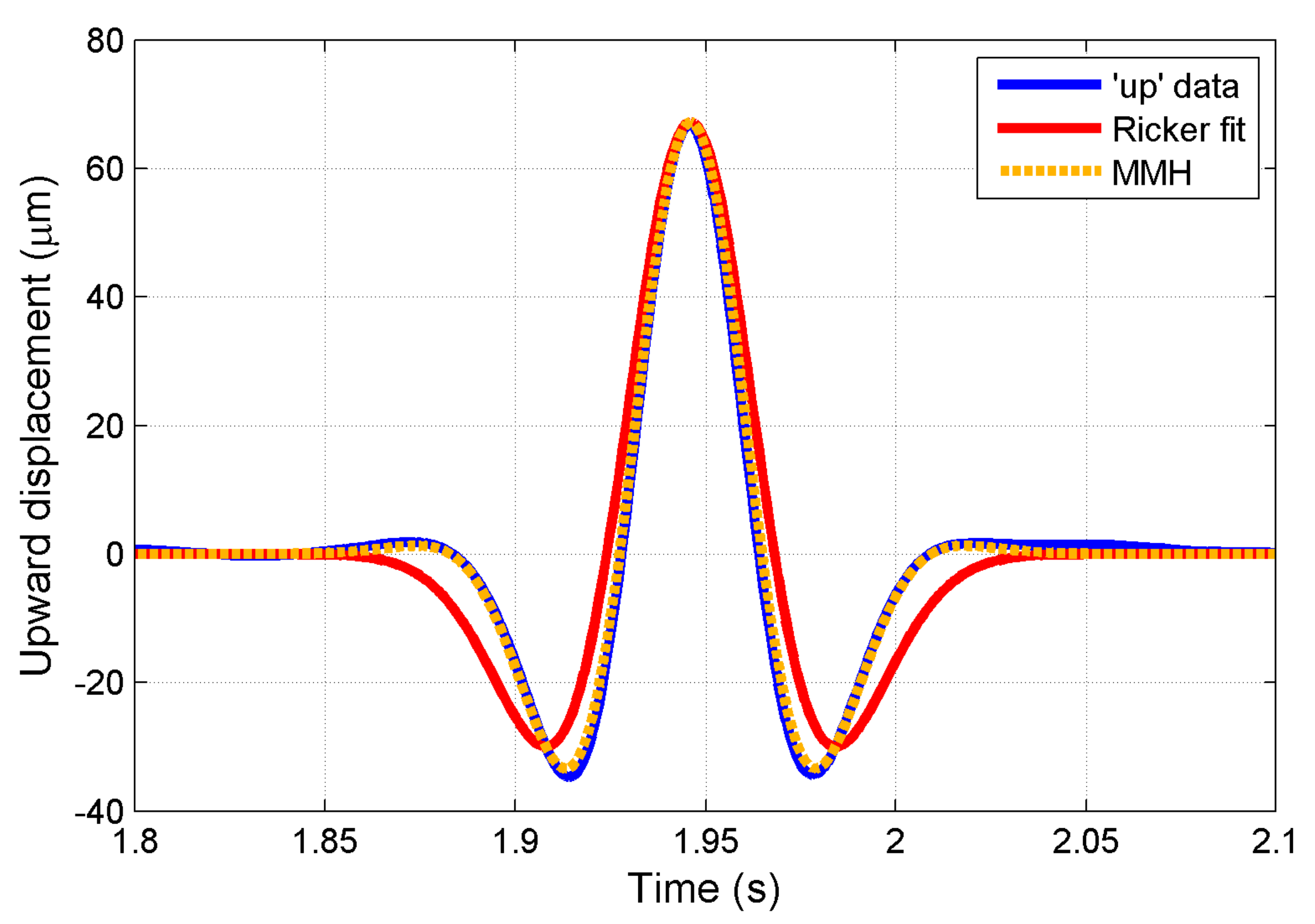
The upward displacement data (blue) of Figure 3 is plotted around the peak time of 1.946 s after the start of this FE dry run, coded sgr9a, with V_s = 128 m/s, τ = 40 ms, and g_r = 4 s⁻¹. It used node 2162 at 222 m radius, chosen to provide a symmetric hump form. Additional plots show the Ricker form (red) and an improved mathematical form (dotted orange), representing a Morphing Mexican Hat shape (MMH), the function shown in Equation (4), which is a combination of two terms from the Hermite polynomial sequence.

Compared with the Ricker form (R_k), the FE data shows additional zero crossings which are provided by the fourth-order Hermite polynomial, the second derivative of the Ricker function, R_k′′. A combination of terms provided a better fit with extra zero crossings. Other combinations of terms may prove useful in the analysis of more complex seismic wavelets where more zero crossings are created as the energy is dispersed both spatially and in time.

7. The Morphing Nature of the Wavelet Structure

FE animations of the travelling wavelet show a morphing structure changing at approximately 1.5 Hz (for g_r ≈ 4 s⁻¹) from a “hump” to a “dip” and back, with the symmetric hump being periodically inverted via antisymmetric forms. This dynamic wavelet structure is described here as a “Morphing Mexican Hat”, or MMH function (Figure 3 and Equation (4)), which is a combination of two derivative functions R_k and R_k″ of the scaled and offset time T (Equation (1)).

A good fit was found when the two components were scaled to have equal value at T = 0.

$$R_k\prime (T)=K{e}^{\frac{-T^2}{2}}(-3T+T^3)$$

(2)

$$R_k″(T)=K{e}^{\frac{-T^2}{2}}(-3+6T^2-T^4)$$

(3)

$$MMH(T)=\frac{(3R_k(T)-R_k″(T))}{6}=K{e}^{\frac{-T^2}{2}}(6-9T^2+T^4)/6$$

(4)

The MMH function zeroes are determined by a quadratic in T², yielding T² = 0.725 or 8.275, and T = ±0.8515 (inner zeroes) or T = ±2.877 (outer zeroes). Once this fit to the zeroes was found, the intervening shape fitted the data well, to provide a better understanding and prediction of this special interface wave and its morphing process.

8. The FE Forcing Pulse Drivers

In much of the recent work a Ricker driver pulse has been used. The two parameters K and τ, as set by the forcing pulse, control the peak amplitude and the width of the propagated pulse. The peak force is arbitrarily set at 1 MN, but as the FE calculations are linear, this assumption is unimportant. Width τ has more complex effects. The net force is seen to be zero, using the antisymmetric Ricker integral (Hermite polynomial of order 1).

The earlier work [17] used a finite-length polynomial pulse found useful in other applications by one author (PCM), again with a zero/zero width given by τ:

$$F(T)=K{(1-T)}^3{T}^3$$

(5)

where T = t/τ and K = 0 outside 0 < t < τ.

The FE Ricker drive pulse also needs to be truncated and this was done at t = t₀ ± 4τ when the residual amplitude is less than K/10¹².

9. Modeling Comparisons with FE (PAFEC) and Wavenumber Integration (OASES)

The “OASES” procedure (Ocean Acoustics and Seismic Exploration Synthesis) [27] uses the wave number integration method, also known as the Fast Field Program (FFP), to solve the wave equation using the Green’s function [28,29,30,31,32] as a function of depth in a stratified media, where the physical properties vary only with depth. The integration is then performed over the wave number range using a Fast Fourier Transformation. An approximation made with the wave number integration method is to use the asymptotic form of the Hankel function, limited to conditions with small changes over distances less than a wavelength. OASES is widely considered to be the de facto standard for underwater propagation loss prediction, especially in range-independent channels as the wavenumber integration solution is an exact solution even with an elastic seabed.

It is useful to compare an FE (PAFEC code supported by Pacsys Ltd., Nottingham, UK) simulation with OASES to verify that the two very different numerical models are in agreement in dealing with wave propagation near the water and sediment interface. A Scholte wave with suitable environmental parameters was generated in simulations with the numerical models for a comparison here. The underwater channel used had a water depth of 32 m over 100 m depth of seabed sediment. There was a maximum range of 200 m for PAFEC, and semi-infinite seabed with a maximum range of 250 m for OASES with constant compressional and shear wave speeds. The sound speed in water is 1500 m/s, and water density is 1000 kg/m³. The compressional wave speed is 1520 m/s and shear wave speed 128 m/s in the sediment.

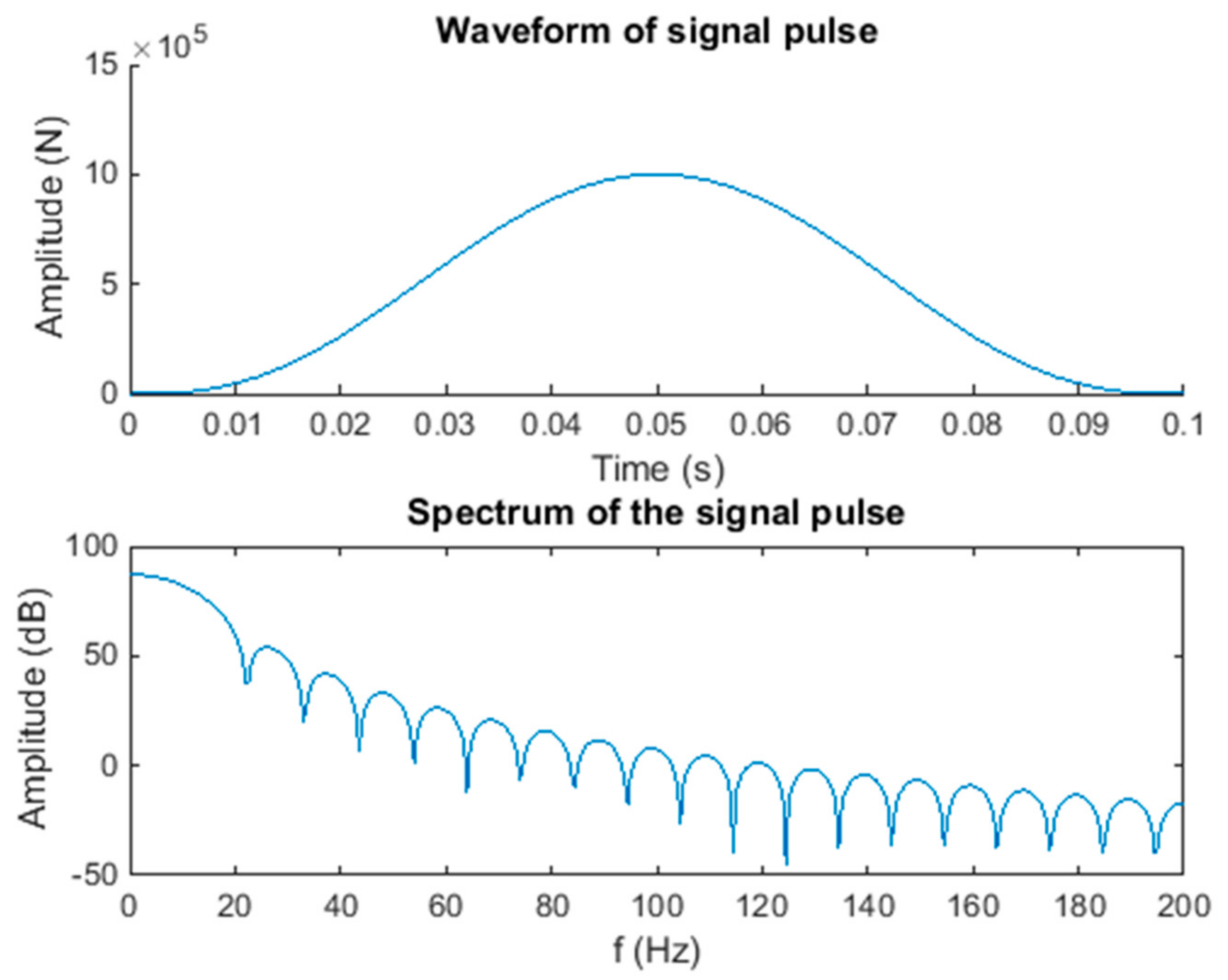
The source used in the simulation was a polynomial impulse force with a pulse duration of τ = 0.1 s, as shown in Equation (5). The time domain PAFEC analysis used transient time steps of 0.1667 ms. OASES is a frequency domain model. The frequency band used here is from 0 Hz to 200 Hz. The waveform and spectrum of the source signal are plotted in Figure 4. The spectrum is on a log scale. It is noticed that the signal amplitude at 200 Hz is about 105 dB less than the maximum at f = 0 Hz. The signal energy in the main lobe of the signal is 99.97% of the total energy. The width of the main lobe is about 22 Hz. This implies that the bandwidth of the simulation with OASES can be reduced substantially.

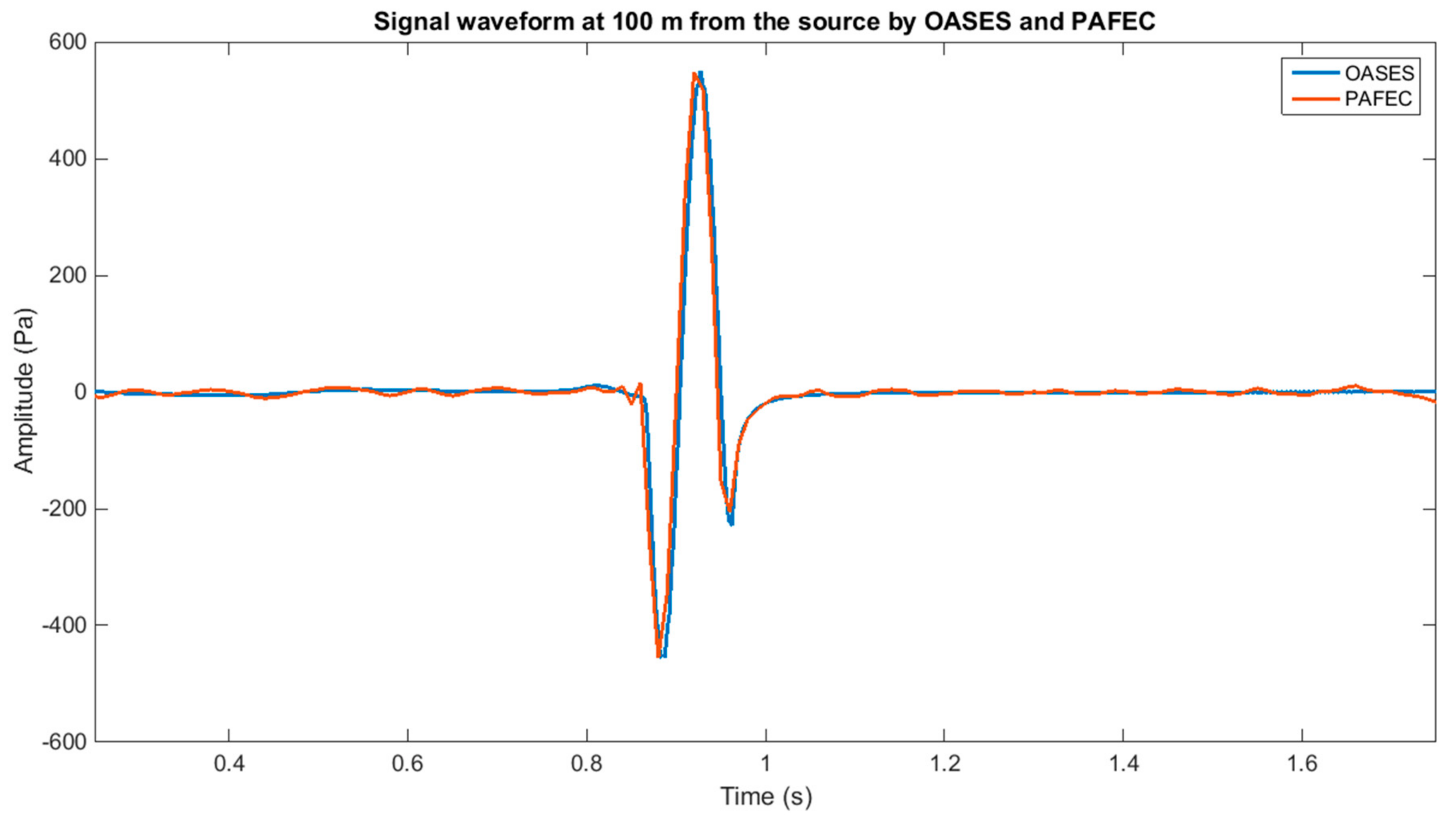
Both PAFEC and OASES were used to calculate the acoustic pressure as a function of range and time close to the water and seabed interface in the water column in order to demonstrate the Scholte wave.

An impulse signal was applied in a vertical direction onto the water and sediment interface to generate a response in OASES simulation. The impulsive response was then convolved with the polynomial pulse to generate a time domain signal of pressure. The polynomial impulse was applied directly in PAFEC to generate the same pressure signal.

The agreement seen in Figure 5 between the two methods is very good. Nevertheless, it can be seen that there are some additional signals, albeit with much smaller amplitudes, before and after the main pulse in the middle in the PAFEC simulation.

The theoretical Scholte wave speed is 115.9 m/s [33,34] with the parameters used. The plots in Figure 3 indicate that the predicted speed of the Scholte wave by PAFEC is slightly faster than that by OASES. The estimated speed from the simulations is 115.7 m/s by OASES and 116.1 m/s by PAFEC. Both are very close to the theoretical value.

10. The Retention of Wavelet Energy Is Key to the Optimal Transmission

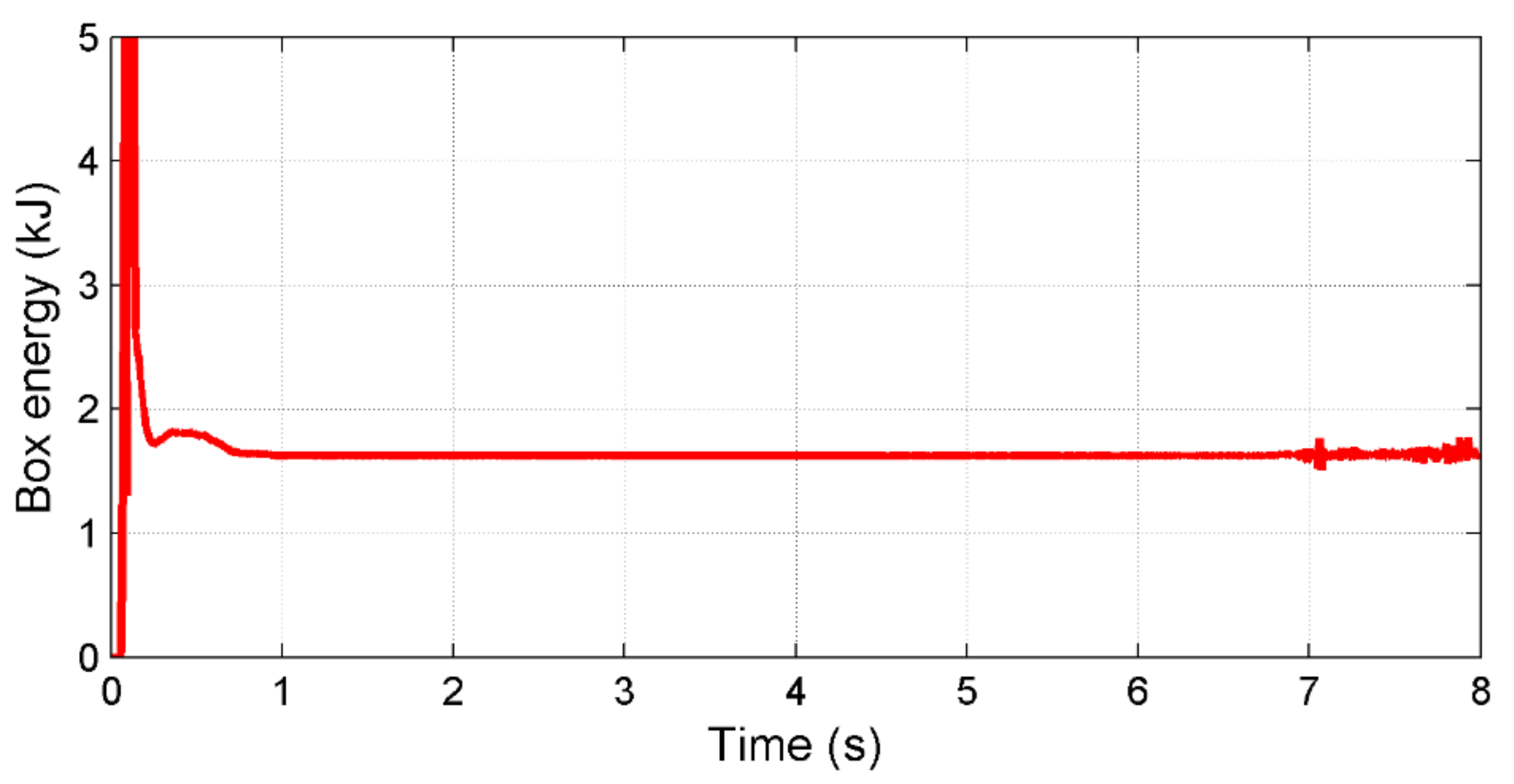
In Figure 6 the stability of the wavelet energy has been computed by defining an energy box, wherein the elastic energy can be calculated by a special FE procedure. This energy box travels with the wavelet as the transient analysis progresses and includes the energy within all azimuth directions for this axisymmetric model, so that a constant value indicates a cylindrical spreading of intensity, seen to extend to over 850 m in range. The travelling box size (8 m deep by 16 m radially) was set after studying the animation produced by the FE. The procedure also required a precise wavelet speed at 123.86 m/s (estimated error < 0.1%) for this dry model. The Ricker zero-to-zero drive pulse width (τ) was 25 ms, with V_s = 128 m/s at the interface and g_r = 4 s⁻¹.

Static energy is stored as the pulse is initiated, but the energy computed diminishes as the energy box moves away from the origin. The propagating energy also shows some changes in the first second as a separate mode travels outwards more rapidly than the main wavelet. The box energy then stabilises (1627 J ± 1 J) until some FE-induced reverberation is seen after 7 s, when the wavelet has travelled out to over 850 m range.

11. Stability of the Wavelet Shape

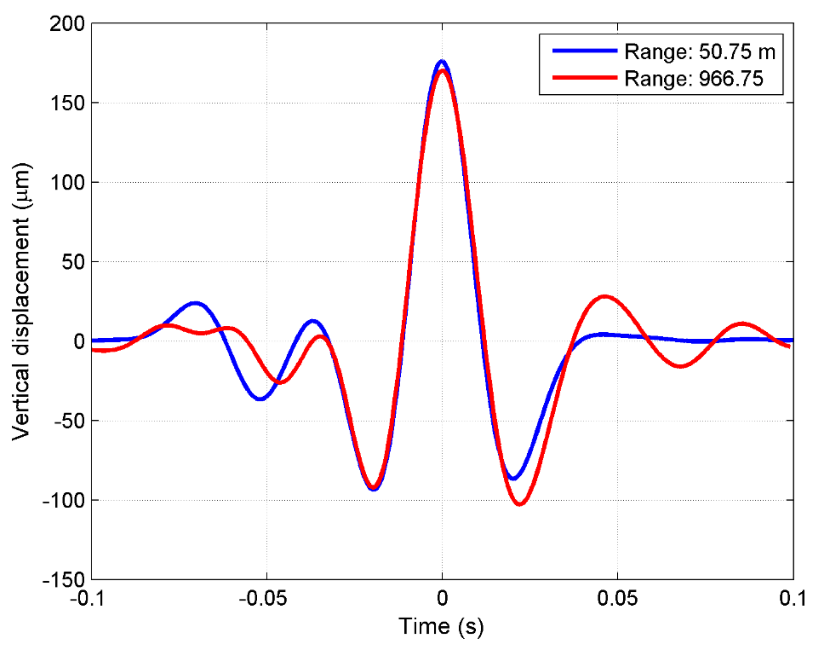
The spatial shape displayed in Figure 2 shows displacement data versus position, but more precise numeric data can be obtained as displacement against time. Data from a chosen FE node (e.g., a junction between two finite elements) gives the time series shape.

Figure 7 shows that whilst the MMH mathematical form can fit early wavelets well, they slowly expand in time, with their energy being dispersed over a longer period, but without launching a separate mode with higher group speed. This slow expansion of the wavelet with increased zero crossings is typical of seismic data but is here insufficient to escape the energy box, as it has not produced a separate faster mode (as seen in Figure 6).

The FE model did not consider absorption (conversion into heat) which is likely to limit the range in practice. However, data presented by Jensen et al. [35] from measurements of seabed vibration generated by seabed explosion charges (up to 0.72 kg) showed results detectable at over 2 km range. These results showed many zero crossings (>10) within a coherent wavelet group, propagating in sediment with an “inferred shear speed gradient of ~4 (m/s)/m”.

12. The Shear Speed Gradient Controls the Morphing Frequency

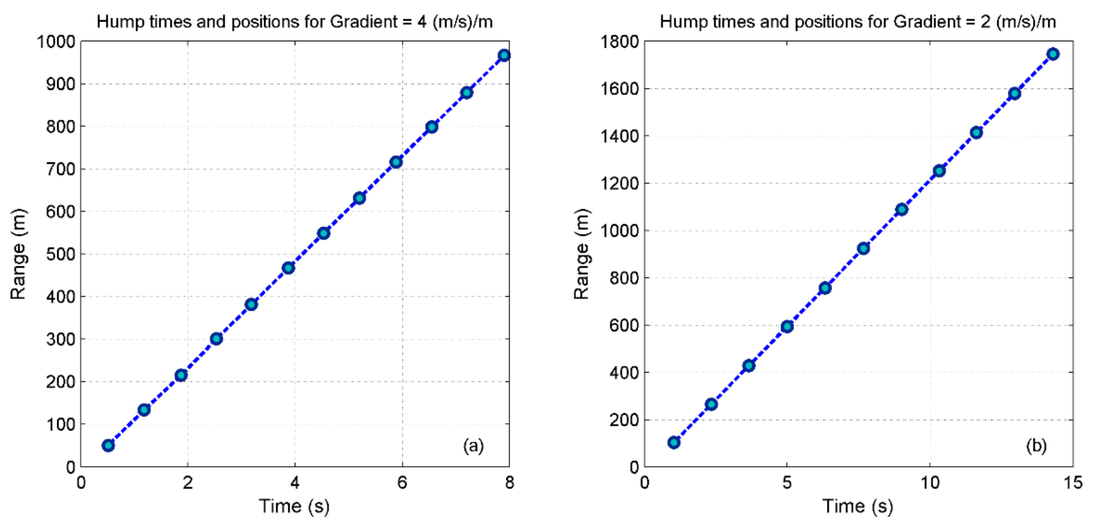
The frequency of the morphing cycle (hump to dip and back) is controlled by the shear speed gradient. In Figure 8, the ranges of the 11 nodes from node 1680 to node 9002 are plotted against the times at which the humps occur.

When g_r = 4 s⁻¹ (or (m/s)/m) the morphing cycle takes 0.67 s, a frequency of 1.488 Hz, with humps occurring every ~83 m. When the gradient is reduced to 2 s⁻¹, the morphing frequency is reduced to 0.748 Hz. For the second run, the overall range was doubled, using larger elements and a slower transient step rate. However, the vertical mesh density was retained, thus checking that the results were not sensitive to the element proportions. Over this range, the morphing frequency, f_m, is then given by f_m ≈ 0.37 g_r.

This factor is unitless, as the shear speed gradient, g_r, has units of s⁻¹. Checks made using other gradients show in

Table 1. The variation of the morphing frequency with the shear wave speed gradient.

Shear Speed Gradient (s−1)	1	2	4	8	16	32
Morphing frequency (Hz)	0.335	0.748	1.488	2.912	5.682	10.91

that this trend is only approximately linear.

13. Wavelets in a Hamilton Profile FE Model Are Also Seen to Morph Regularly

The work published earlier [17] using a shear speed depth profile from data published by Hamilton [21] and the polynomial force function of Equation (5) gave more complex wavelet shapes. However, the intriguing morphing characteristic was clear within the animated results presented at various conferences by Hazelwood [36,37].

Figure 9 shows results from the earlier FE model pwb42, based on the Hamilton data. The wavelet speed is 110 m/s with a morphing frequency of 1.9 Hz.

14. The Variation of Group Velocity with Wavelet Width

In order to study the small variation of speed of the wavelets with the drive pulse width τ, a special procedure was developed. The morphing form makes it more difficult to assess the wavelet speed (or group velocity).

Initial FE runs were inspected to determine the timing of a pair of hump forms. Suitable nodes were then allocated for a second FE run wherein their detailed response times were stored and later recovered. Speeds in

Table 2. Wavelet properties taken from runs with different Ricker drive pulse widths.

	Pulse Width Tau ms	Transit Speed ms−1	Z/z Width #1 ms	Z/z Width #2 ms
1	16	117.89	15.4	16.6
2	20	117.74	18.8	20.4
3	25	117.5	23	24
4	32	117.38	29	29
5	40	117.39	36	36
6	50	117.60	45	45
7	64	117.92	56.3	58
8	80	118.79	70.4	74
9	100	119.47	86	88

are determined between two symmetric humps, and their expanding widths were measured as times between their zero crossings (z/z widths #1 and #2). These were all full wet runs, with the water elements included. This data is also plotted in Figure 10.

This data, plotted in Figure 10, show a minimum group velocity at about 36 ms.

15. Reduction of the Wavelet Peak with Time and Distance

The improved wavelet shape with the Ricker pulse drive made a better analysis of peak intensity versus range possible. The peak vertical displacement Zp at the hump stage followed a close approximation to the cylindrical spreading rule. If perfect, there would be a constant product of range with displacement squared, described here as an “intensity volume”, to distinguish it from the pressure squared used in air acoustics.

Acoustic intensity represents the energy being propagated and for compression waves can be given as the square of the acoustic pressure, when other terms (such as material properties) are constant. Rather than calculating the complete elastic energy as was done by the energy box procedure, the peak vertical interface displacement at the hump stage (when there is little horizontal displacement) can be squared for the same purpose.

Rather than providing an energy density per unit area, the result represents the energy per unit length of the wave front, and when multiplied by the radius gives the propagating energy as a volume, proportional to the volume displaced by the whole central peak (zero to zero) with no absorption. The loss of this intensity is shown in Figure 11.

A loss of about 9% in the propagation to 1.6 km radius for this dry model shows the departure from a cylindrical spreading rule, to be compared with the much smaller loss of energy within the energy box of about 0.1%. The peak intensity loss has not created a separate wavelet with a different speed but rather spread the wavelet energy within the travelling box, with additional zero crossings.

16. Comparison with Other Seismic Surface Waves

Similar plots of group velocity variation with pulse width are associated with seismic records which are described as an “Airy phase” by Shearer [38]. Extreme examples are the “long period” (typically 20 s) waves, created by earthquakes, which circumscribe the Earth up to three times before becoming undetectable in noise. The concentration of energy which occurs at a turning point (a maximum or a minimum) in the group velocity dispersion plot creates these dominant forms. Earthquake data over 10 years was analysed by “stacking”, a seismologists’ statistical technique used to display signals otherwise buried in noise. The propagation of these long-period wavelets is linked to the graded layers of the Earth, as described by Fowler [39].

17. Matching the FE Outward Displacement Data to the Ricker Mathematics

Figure 12 shows that the horizontal displacement, radially outward, from the FE model data used for Figure 3, is a good fit to a suitably scaled differential function Rk′. There are 3 zero crossings visible in the data, matching the cubic term in the equation. Larger discrepancies are seen near the peaks than occurred in Figure 3 data, but the fit has proved adequate for a hodograph analysis of the morphing process.

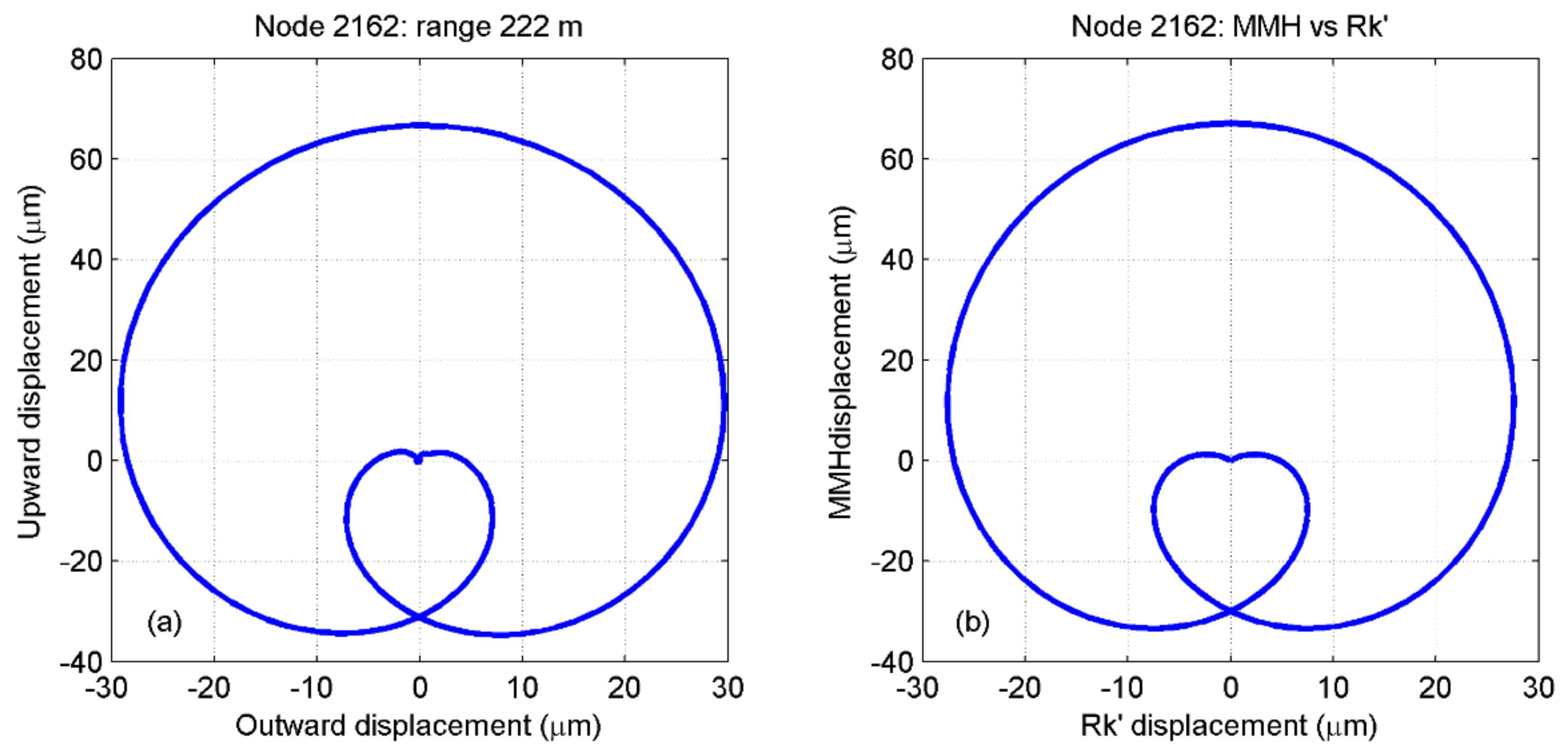
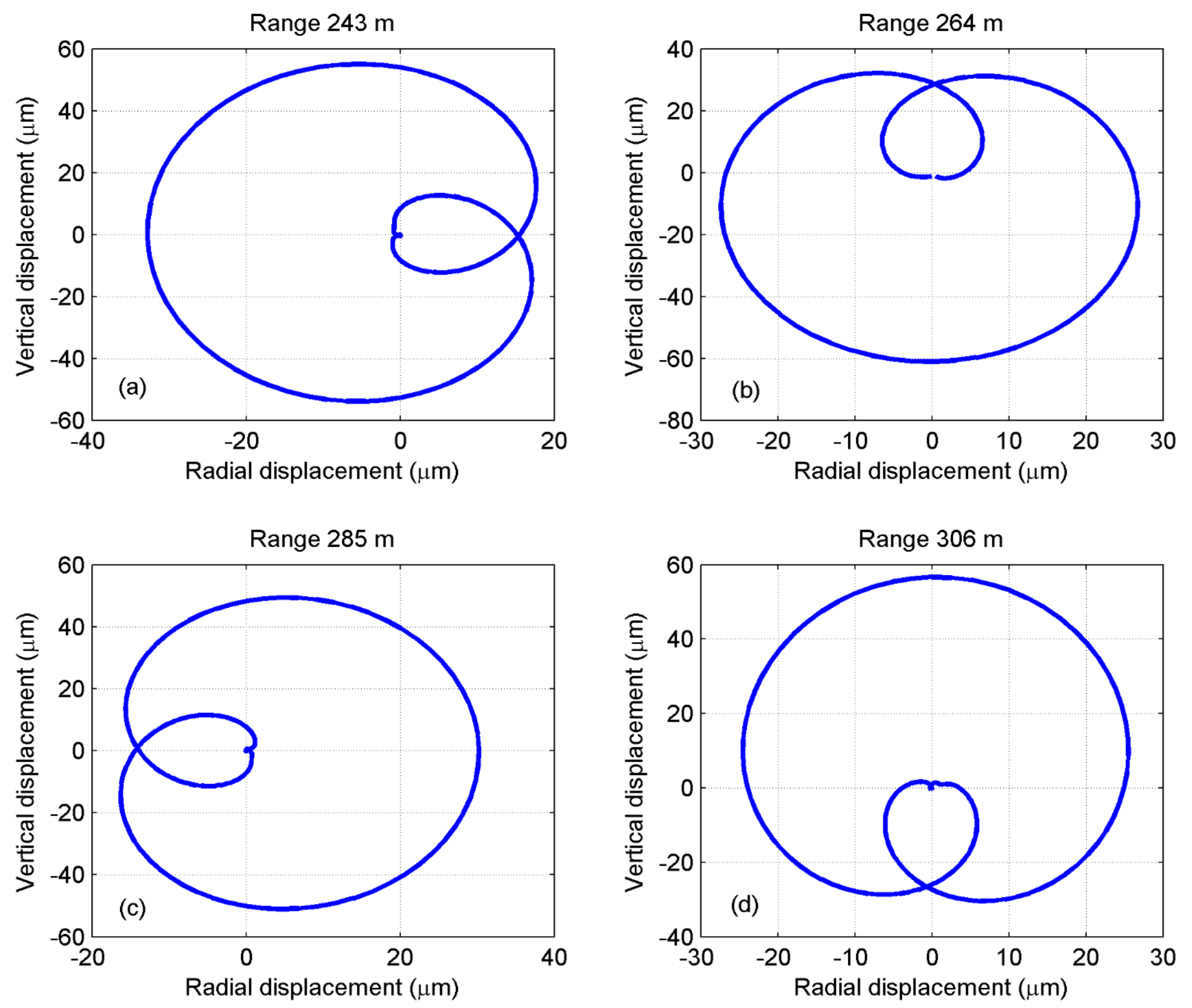
18. Presenting the Data as a Hodograph—The Orthogonal Motion

In Figure 13 the horizontal radial motion and vertical motion are plotted on different axes. Such plots are called hodographs by seismologists. The crossover point was used to identify the best node at which to sample the FE data. The second plot uses analytic data.

A separate analysis was made after run sgr9a for each of the surface nodes 2162, 2246, 2330, 2414, and 2498, which are 21 m apart at ranges from 222 m to 306 m. Figure 13 shows the last four, with data for node 2162 (at 222 m) having been used for Figure 3 and Figure 12.

19. Using Hodographs to Observe the Morphing Process

The data of Figure 14 can be viewed in the hodograph figures in Figure 15, showing a symmetry which rotates as the MMH wavelet morphs.

Note that the horizontal extreme excursions remain about half of those vertically. This rotation process provides further information on the nature of the MMH wavelet.

20. The Morphing Mathematics

The displacement data as shown in intermediate hodographs can be predicted by the use of a rotational coordinate transform matrix. Matrices can be used to convert Cartesian coordinates from one frame into another. A rotation in the x, y plane converting coordinates x₁, y₁ to x₂, y₂ is given as a function of the Euler angle, θ, (Wertz [40]).

$$\left(\begin{array}{c}{x}_2\\ y_2\end{array}\right)=\left(\begin{array}{cc}\hspace{0.17em}\hspace{0.17em}\hspace{0.17em}\cos \theta & \sin \theta \\ -\sin \theta & \cos \theta \end{array}\right)\left(\begin{array}{c}{x}_1\\ y_1\end{array}\right)$$

This matrix can rotate hodograph coordinate data displays to a new angle θ, which represents a delay. A rotation of θ = 360° represents a complete morphing cycle from hump to hump, as seen in Figure 15. The time series of vertical and horizontal data at any intermediate morphing condition can then be calculated.

21. Wavelet Morphing in a Moving Frame Provides Sinusoidal Vibration Functions

The hodographs provide two-dimensional views of displacement coordinates from a fixed point, as plotted over time at a particular radial distance. However, it is also possible to plot the displacements as observed at positions within a moving window, arranged to track the wavelet position. Results from this moving frame transformation, which has been tested using the FE data, yield continuous sinusoidal motions at the morphing frequency. The window, similar to the “energy box” used for Figure 6, tracks the wavelet, maintaining a concentration of energy at its centre. Other properties of the MMH wavelet can be studied with FE analysis such as the detailed water motion studied in the earlier paper [17].

22. Conclusions

This further investigation into the seismic vibrations created by piling and dredging has helped to explain the nature of the measurements in the field by looking at idealised versions of the sedimentary seabed. Some aspects of the underlying physics are thus exposed. The frequently complex dissipation of energy is reduced for this simple form with an optimal propagation providing a worst case from the environmental perspective.

More studies of the propagation of vibration energy from piling activities will be needed to estimate the environmental impact of these and other similar real operations. Currently the water-borne acoustic outputs are being assessed in a sequence of conferences [41], but the effects of vibration on the benthic life may be found to be as significant. They can be linked to the improved techniques for measurement of the water particle velocity and the sensitivity of benthic fauna to this energy form.

The mathematics of the fit found here to the wavelets produced in this new half-space physical model are relatively simple. These may be found relevant to a variety of fields such as environmental noise, seismology, and bioacoustics. As predicted in the previous paper [17], the elliptical particle motion within these seismic wavelets provides a mechanism whereby benthic creatures could resolve the direction of their propagation.

Future work should include further studies of measurements using various saturated sediments for comparison with predictions based on the results presented here.