Numerical Simulation and Uncertainty Analysis of an Axial-Flow Waterjet Pump
by
 ,
,
Ji-Tao Qiu
1, 
Chen-Jun Yang
1,*,
Xiao-Qian Dong
1,
Zong-Long Wang
2,
Wei Li
1 and
Francis Noblesse
1 1
State Key Laboratory of Ocean Engineering, Collaborative Innovation Center for Advanced Ship and Deep-Sea Exploration, Shanghai Jiao Tong University, Shanghai 200240, China
2
Marine Design and Research Institute of China (MARIC), Shanghai 200011, China
*
Author to whom correspondence should be addressed.
J. Mar. Sci. Eng. 2018, 6(2), 71; https://doi.org/10.3390/jmse6020071
Submission received: 30 March 2018
/
Revised: 1 June 2018
/
Accepted: 5 June 2018
/
Published: 11 June 2018
(This article belongs to the Special Issue Marine Propulsors)
Abstract
:Unsteady Reynolds-averaged Navier–Stokes simulations of an axial-flow pump for waterjet propulsion are carried out at model scale, and the numerical uncertainties are analyzed mainly according to the procedure recommended by the twenty-eighth International Towing Tank Conference. The two-layer realizable k-ε model is adopted for turbulence closure, and the flow in viscous sub-layer is resolved. The governing equations are discretized with second-order schemes in space and first-order scheme in time and solved by the semi-implicit method for pressure-linked equations. The computational domain is discretized into block-structured hexahedral cells. For an axial-flow pump consisting of a seven-bladed rotor and a nine-bladed stator, the uncertainty analysis is conducted by using three sets of successively refined grids and time steps. In terms of the head and power over a range of flow rates, it is verified that the simulation uncertainty is less than 4.3%, and the validation is successfully achieved at an uncertainty level of 4.4% except for the lowest flow rate. Besides this, the simulated flow features around rotor blade tips and between the stator and rotor blade rows are investigated.
1. Introduction
Due to high propulsive efficiency and superior cavitation performance, waterjet propulsion is particularly suited for high-speed crafts. In recent years, it has been gradually applied to large-scale ships; in such cases, it becomes important to accurately evaluate the hydraulic performance of the pump in order to predict the ship’s powering performance correctly. The waterjet propulsion pumps have been designed by means of potential flow-based theoretical methods since the last century. To improve the cavitation performance of the rotor, experimental and numerical investigations are often conducted to analyze the tip-clearance flow apart from optimizing blade loading distribution and section profiles. With the rapid advances in computer hardware capability and CFD software technology, viscous flow simulation has increasingly become preferred to assist in designing the waterjet propulsion pumps, as it is capable of providing more detailed and realistic flow information in addition to more accurate hydraulic performance predictions than those by potential flow methods. Meanwhile, however, the reliability of CFD simulation has become an issue that has drawn increased attention from both research and design communities. Starting with the convergence study of discretization scheme and grid size, the theories and methodologies are gradually being developed for analyzing the numerical uncertainty in CFD simulation.
In 1998, the American Institute of Aeronautics and Astronautics (AIAA) presented the first CFD uncertainty analysis procedure [1], which consists of two processes: verification and validation (V&V); Roache [2,3] published a monograph on CFD uncertainty analysis, and proposed the grid convergence index (GCI) method for verification with at least two sets of grids. In 1999, the 22nd International Towing Tank Conference (ITTC) [4,5] introduced a preliminary procedure for CFD uncertainty analysis based on the work of Stern et al. [6] and Coleman et al. [7], where the generalized Richardson extrapolation (RE) approach [8] was employed to evaluate the uncertainty of numerical simulations. In 2002, according to the GCI method, the 23rd ITTC revised the procedure by including the safety factor approach in the existing ITTC procedure [9]. In 2017, the 28th ITTC introduced the least squares root (LSR) method for error estimation [10] based on the studies by Eça et al. [11] and Larsson et al. [12]. Besides this, Shen et al. [13] discussed the probability distribution of CFD simulation results, analyzed the sources of numerical uncertainty, and proposed an uncertainty analysis method based on orthogonal experiment design and variance analysis.
Simonsen et al. [14] conducted an uncertainty analysis of steady Reynolds-averaged Navier–Stokes (RANS) simulations for the tanker Esso Osaka in straight-ahead, pure drift, and static rudder conditions according to the procedure proposed by Stern et al. [15]. As far as the resistance and hydrodynamic moments are concerned, the analysis results for the appended hull indicate that the validation is at a high level but not achieved for all the cases investigated. Zhang et al. [16] simulated the SUBOFF submarine model by using three sets of successively refined grids and analyzed the numerical uncertainty of hull surface pressure distributions according to the ITTC procedures. Yang et al. [17] analyzed the numerical uncertainty due to grid size in the CFD simulation of an open-water propeller according to the ITTC procedures and investigated the effects of turbulence models. It is noted that, as ships and propulsors have a complex geometry, extremely fine grids (and time steps for unsteady flows) are needed in order for the solution to fall in the asymptotic range. Limited by hardware resources, three sets of grids are typically used for the RE-based analysis, and it seems difficult for the solution to reach the asymptotic range in complicated three-dimensional flows.
The uncertainty analysis can be done more rigorously for two-dimensional flows around simple geometries. Rosetti et al. [18] simulated the unsteady flow around a two-dimensional circular cylinder over a large range of the Reynolds number using five sets of grids and five time-step sizes and analyzed the simulation uncertainties. It was shown that the differences between numerical and experimental results stemmed from modeling errors instead of numerical ones. Diskin et al. [19] conducted a grid-convergence study of RANS simulations for the NACA 0012 airfoil and a flat plate by using three in-house codes and concluded that establishing an asymptotic converge order was more difficult than expected even with very fine grids. The authors also found that the grid resolution in the vicinity of geometric singularities, such as pointed leading/trailing edge, was essential to improve the accuracy and convergence property of CFD simulation.
The internal flow of the axial-flow pump is complicated due to the clearance flow around rotor tips and the unsteady interaction between rotor and stator blade rows, and the fidelity of CFD simulation results may influence the designer’s judgment of the pump’s cavitation performance. Therefore, the analysis of numerical uncertainties is very important, but the related research work is insufficient to date. In this work, unsteady flow simulations of an axial-flow pump for waterjet propulsion are carried out at model scale by solving the unsteady Reynolds-averaged Navier–Stokes (RANS) equations, and the numerical uncertainties are analyzed mainly based on the procedure recommended by the 28th ITTC [10]. Typical operating conditions are selected for the evaluation of the numerical uncertainties arising from spatial and temporal discretization. Besides this, the simulated flow features around rotor blade tips and between the stator and rotor blade rows are investigated.
2. CFD Uncertainty Analysis Procedure
The uncertainty analysis procedure recommended by the ITTC assesses CFD uncertainty at a 95% confidence level, i.e., the probability that the interval (−U, +U) contains the error δ is 95%, where U is the magnitude of uncertainty. Mainly based on the ITTC procedure [10], the V&V processes that are specific to the present problem are detailed in this section.
2.1. Verification
Verification is a process for estimating the uncertainty and error in numerical simulations which assesses whether the modeling equations have been solved correctly [20]. Being defined as the difference between a simulation result S and the truth T, the simulation error δS is composed of the numerical error δSN and the modeling error δSM, viz, δS = S − T = δSN + δSM. When a numerical solution falls in the asymptotic range, the δSN can be estimated together with the error contained in that estimate via the corrected approach; otherwise, only the numerical uncertainty USN can be estimated to provide a boundary for the δSN via the uncorrected approach. In this work, only the uncorrected approach is used; details about the corrected approach can be found in [10].
The numerical uncertainty is expressed as
where the subscripts I, G, T and P denote the uncertainties due to iteration, grid size, time step size, and other parameters, respectively. For an axial-flow pump, it is more accurate to simulate the unsteady flow arising from rotor/stator interactions. Then, the uncertainties due to the UG and UT in (1) are replaced by a combined discretization uncertainty UGT that is evaluated by refining the grids and time-step simultaneously at uniform refinement ratios. The USN is alternatively expressed as
In this work, the uncertainty due to other parameters, UP, is not investigated and will be neglected in the present analysis.
The iteration uncertainty UI is defined as
where and denote the maximum and minimum values of simulated results in the last two oscillation periods according to [10]. In this work, however, the iteration uncertainty is estimated conservatively by using the data over a complete revolution of the rotor, since the simulated integral quantities oscillate with time randomly and at high frequencies. Besides, it is necessary to exclude the contributions from the simulated physical oscillations in the integral quantities, although they are usually quite small in magnitude.
For the verification based on three solutions, the convergence ratio R is defined as
where S1, S2 and S3 denote the solutions yielded from fine, medium, and coarse grids and time steps, respectively. The convergence is monotonic when 0 < R < 1 but oscillatory when −1 < R < 0. If |R| > 1 the solutions diverge and the uncertainty cannot be estimated. For monotonic convergence, the RE approach is used to estimate the UGT. For oscillatory convergence, the UGT is estimated by
where SU and SL denote, respectively, the maximum and minimum values in the simulation results. Note that the UGT yielded from (5) is just a rough estimate for the boundary of δSN.
According to the RE approach, the estimated error is calculated by
where r and p denote the parameter refinement ratio and the observed order of accuracy, respectively. The observed order of accuracy is determined by
The correction factor, C, is defined as
where pest is an estimate for the limiting order of accuracy of the first term as the grid and time-step sizes go to zero and the asymptotic range is reached, i.e., C→1. The uncorrected approach is used to estimate the USN only. The UGT is estimated by the following formulae that are proposed by Wilson et al. [21] and recommended in [10],
2.2. Validation
Validation is defined as a process for assessing simulation modeling uncertainty USM by using benchmark experimental data and, when conditions permit, estimating the modeling error δSM itself. This process investigates whether the correct equations are solved [20]. The comparison error E is defined as the difference between experimental data D and simulation result S, i.e.,
The validation uncertainty UV is defined as
where UD denotes experimental uncertainty. To determine whether the validation has been achieved, the comparison error E is compared to the validation uncertainty UV and the programmatic validation requirement Ureqd. If the three variables are unequal to each other, one of the following cases must be true:
- (1)
- |E| < UV < Ureqd
- (2)
- |E| < Ureqd < UV
- (3)
- Ureqd < |E| < UV
- (4)
- UV < |E| < Ureqd
- (5)
- UV < Ureqd < |E|
- (6)
- Ureqd < UV < |E|
In the first three cases, the validation is achieved at the UV level, but the modeling error cannot be estimated as the comparison error is below the uncertainty (noise) level. Particularly, in the first case the validation is successfully achieved at a level below Ureqd.
In the last three cases, the validation is not achieved but the modeling error can be estimated. If |E| >> UV, the modeling error dominates and is approximately equal to E. In case (4) the validation is successful at the |E| level.
3. Unsteady RANS Simulation of an Axial-Flow Pump
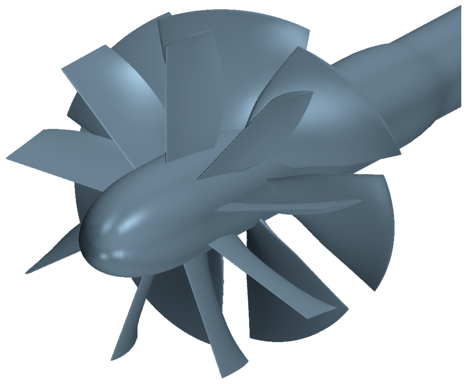
Numerical simulations are conducted for a model-scale axial-flow pump by solving the unsteady RANS equations for incompressible fluids. The pump consists of a seven-bladed rotor and a nine-bladed pre-swirl stator. The shroud diameter d is 300 mm. The tip clearance of the rotor is 0.3 mm. The axial spacing between the rotor and the stator is 30 mm. Figure 1 shows the geometric model of the rotor and the stator.
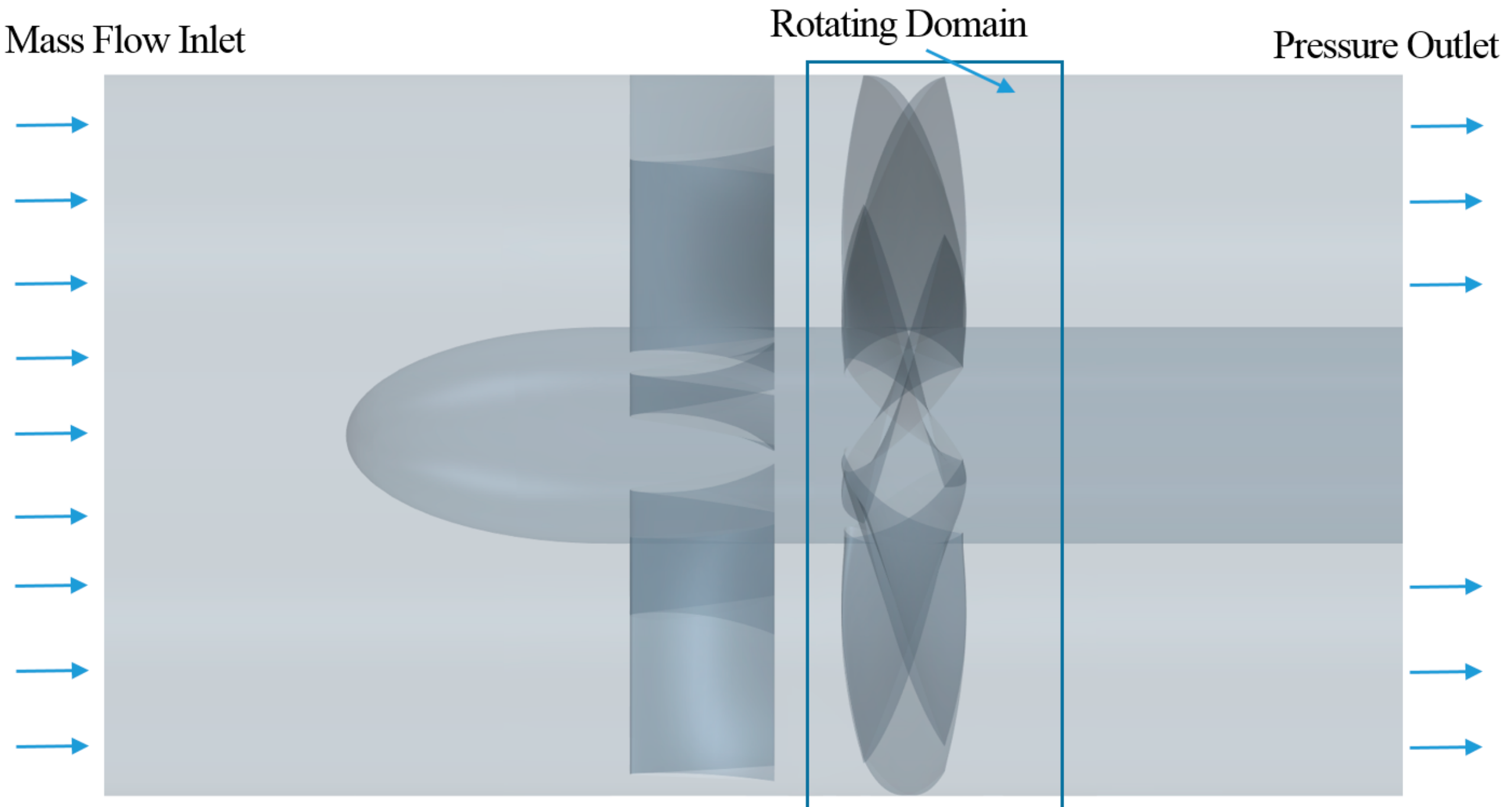
Figure 2 shows the computational domain, which is bounded by a circular cylindrical shroud 16 times d in length. The rotor is located at the longitudinal center of the domain. The rectangular area marked out in Figure 2 is a sub-domain containing the rotor (as well as a portion of the shroud surface and the hub), which is defined in a coordinate system attached to the rotor. The remaining portions of the computational domain are defined in an earth-fixed coordinate system.
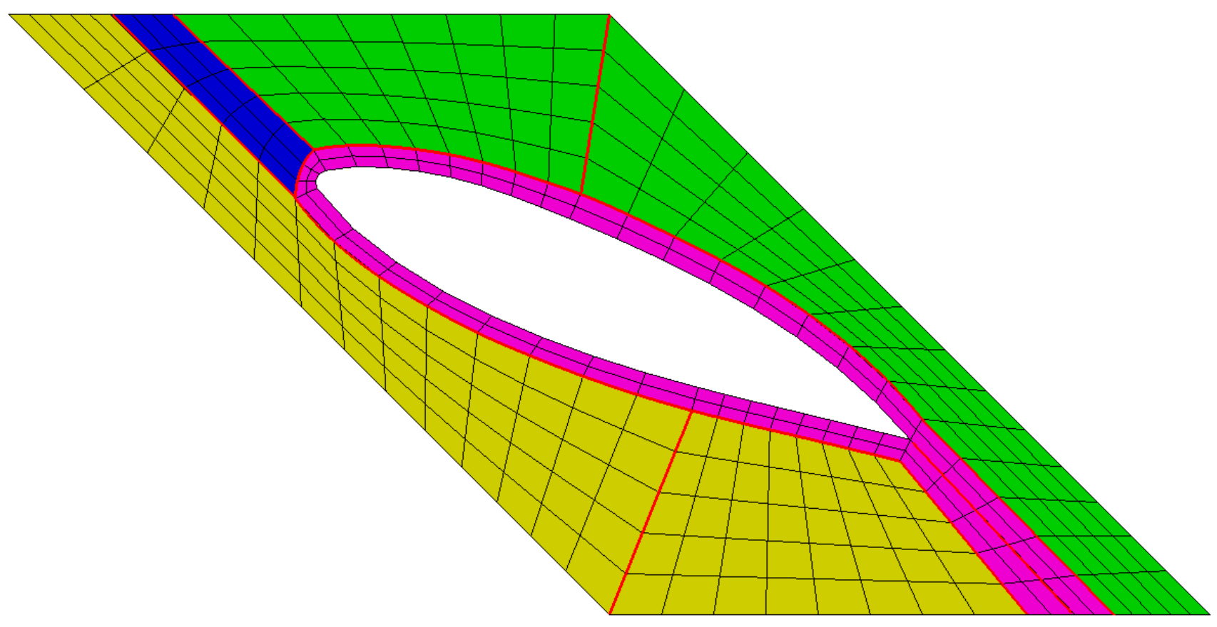
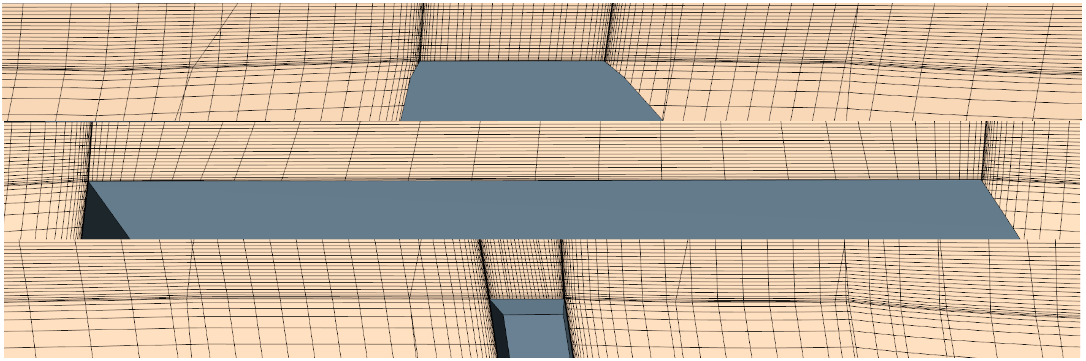
The computational domain is discretized into block-structured hexahedral cells by means of the grid generator ICEM CFD 16.0. Figure 3 illustrates the grid topology around rotor blade sections. The thin area around blade surfaces are discretized with C-grid layers, the area in between the C-grid areas of adjacent blades are discretized with L grids, and the small area upstream of the leading edge is discretized with H grids. The area around stator blade sections are discretized with H grids. In a spanwise direction, H grids are used for both the rotor and the stator. Figure 4 shows the grid structure in the tip clearance of a rotor, which is the same in topology along the chord.
Three sets of successively refined grids are generated with a uniform grid refinement ratio, rG = Δh2/Δh1 = Δh3/Δh2 = , where h3, h2 and h1 denote, respectively, the sizes of coarse grid G3, medium grid G2, and fine grid G1. Figure 5 shows the surface grids for rotor and stator blades. The key parameters of the computational grids are listed in Table 1.
As illustrated in Figure 2, the upstream boundary condition is set as the mass flow inlet, where the flow rate is prescribed; the downstream boundary condition is set as the pressure inlet, where the pressure relative to the reference pressure of the flow domain (atmospheric pressure) is set to zero. All the body surfaces are set as non-slip boundaries. The part of the shroud surface in the rotating sub-domain containing the rotor is set as stationary relative to the fixed coordinate system. At the inlet and the outlet, the turbulence intensity and the turbulent viscosity ratio are set to 2% and 2, respectively.
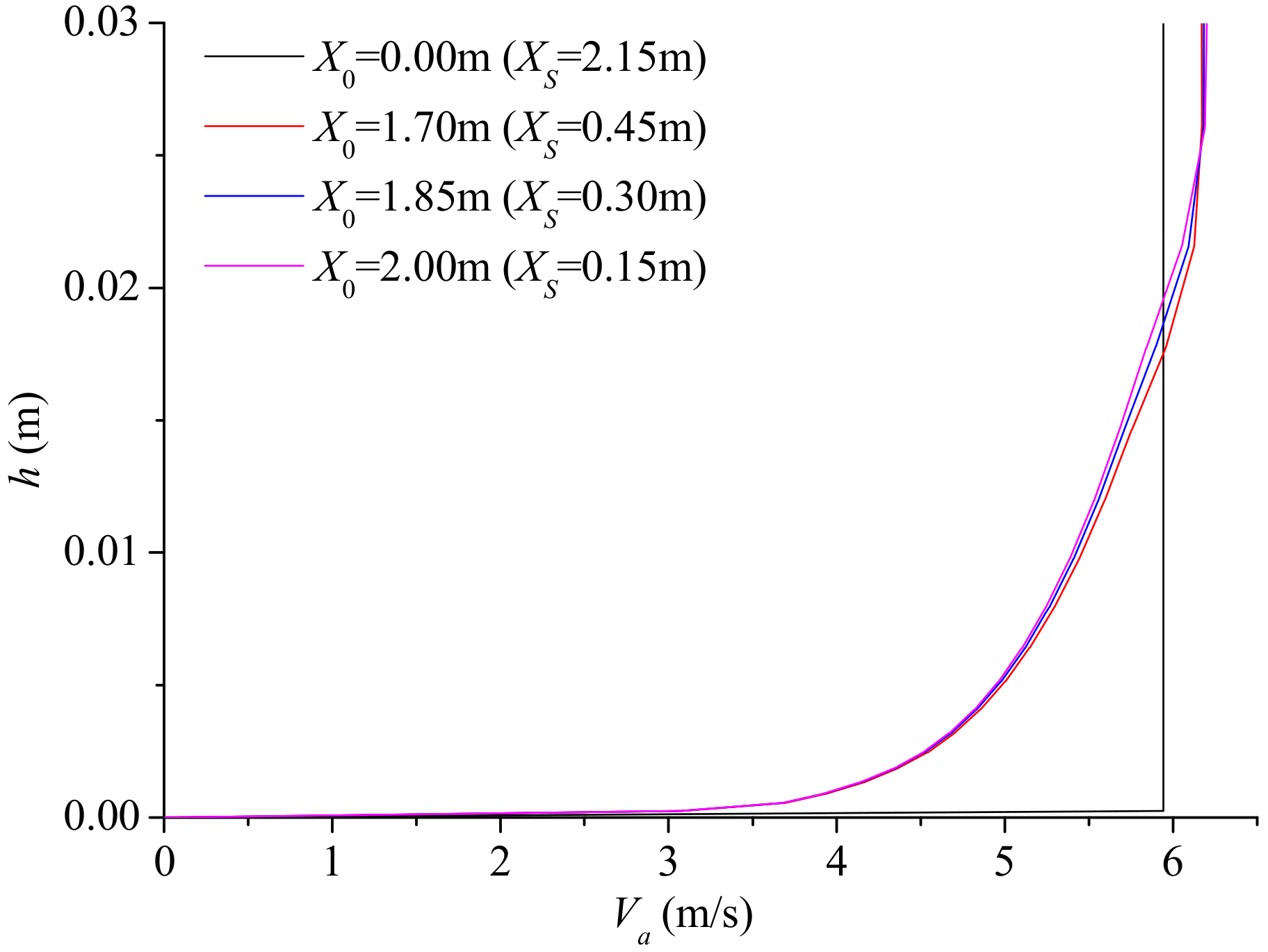
The inlet boundary condition is an issue that can influence the modeling uncertainty in present simulations since the computational domain is just a part of the closed loop used in the pump tests. In our modeling approach, the computational domain is made long enough (16 times the shroud diameter) to allow the boundary layer on the shroud surface to develop fully before the flow arrives at the stator. Figure 6 shows profiles of axial flow velocity Va at three streamwise stations when Q = 0.42 m3/s. It seems that the boundary layer becomes fully developed from 1.7 m downstream of the inlet (0.45 m to the nose of shaft cap), and the inlet velocity profile prescribed by the software would have little influence on the modeling uncertainty.
The unsteady RANS simulations are carried out using the CFD software STAR-CCM+ 12.02. The two-layer realizable k-ε model is used for turbulence closure, and the flow in viscous sub-layer is resolved. The two-layer approach was first proposed by Rodi [22]. As another method of applying the k-ε model in the viscous sub-layer and the buffer layer, it works with either low-Reynolds number type meshes (y+ ~ 1) or wall-function type meshes (y+ > 30). In the layer next to the wall, functions of the y+ are used to specify the turbulent dissipation rate ε and the turbulent viscosity μt. Otherwise, the transport equation for ε is solved. The equation for k is solved across the entire flow domain. The realizable k-ε model was proposed by Shih et al. [23], which consists of a new model equation for the turbulent dissipation rate and a new eddy viscosity formulation. The model was validated for different flow types, including rotating homogeneous shear flows, and found to perform much better than the standard k-ε model.
The governing equations are discretized with second-order schemes in space and a first-order scheme in time and solved by the semi-implicit method for pressure-linked equations (SIMPLE). It would be more accurate to use a second-order scheme for the discretization in time, but convergence problems were encountered when the flow rate was low. To be consistent with the order of discretization accuracy in space [11,24], three time-step sizes having a uniform refinement ratio, rT = Δt2/Δt1 = Δt3/Δt2 = 2, are used in the unsteady simulations, where Δt3, Δt2, and Δt1 denote coarse, medium, and fine time-step sizes, respectively. Note that the grids and time steps must be coarsened or refined simultaneously. To expedite convergence, steady-flow simulations are used to initialize unsteady simulations. In each time step, 20 iterations are performed to reduce the residuals to an acceptable level.
4. Numerical Uncertainty Analysis for the Axial-Flow Pump
The analysis of numerical uncertainty in the present RANS simulations is conducted for the axial-flow pump described in Section 3. Three volumetric flow rates (Q = 0.35 m3/s–0.471 m3/s) are considered which cover a wide range of the pump’s operating conditions. The uncertainties in the simulated head and power are evaluated.
The head H and power P of a pump are defined as
where pd and pu denote shroud-surface pressures averaged over the circumferences at 2d downstream and 2d upstream of the rotor, respectively; Vd and Vu denote the axial velocities averaged over the shroud cross sections at 2d downstream and 2d upstream of the rotor, respectively. The locations where the pressures and axial velocities are numerically evaluated are the same as those in the experiments for the pump model considered here. In (12) the gravitational acceleration and the density of water are denoted by g and ρ, respectively; the torque and the rotational speed (r/min) of the rotor are denoted by M and N, respectively.
4.1. Verification
The rotational speed of the rotor is set to 1450 r/min for the three flow rates considered, which is same as that in the model experiments [25]. The Reynolds number based on the relative inflow speed and the chord length at 0.7Rtip is 2.3 × 10⁶, where Rtip is the tip radius of the rotor. The coarse time step size Δt3 is set to 1.1494 × 10⁻⁴ s, which corresponds to a blade angular displacement of 1° per time step. The medium and fine time step sizes, Δt2 and Δt1, correspond to 0.5° and 0.25° blade angular displacement per time step, respectively. To resolve the flow in viscous sub-layer, the near-wall grid layers need to satisfy y+ ~ 1. Corresponding to the grid sizes as listed in Table 1, the ranges of surface-averaged y+ are given in Table 2 for the flow rates simulated. Figure 7 shows the limiting streamlines on rotor and stator blade surfaces when Q = 0.42 m3/s. On rotor blade surfaces, flow separation occurs mainly on the suction side, in inner radii and close to the trailing edge. On stator blade surfaces, the flow is converging on the suction side but diverging on the pressure side; flow separation occurs on the suction side only, in close proximity to the trailing edge, and from about 40% span to the tip. It seems that the stator blade geometry may need to be improved. The flow patterns simulated with the coarse grid G3 and the fine grid G1 are quite similar to each other.
Figure 8 shows an example of the residuals in the last few time steps before convergence. The residual in continuity drops to 10−5–10−6, those in velocity components to 10−5–10−7, and those in k and ε to 10−6–10−8 when the solution converges. The speed of convergence is slow at low flow rates.
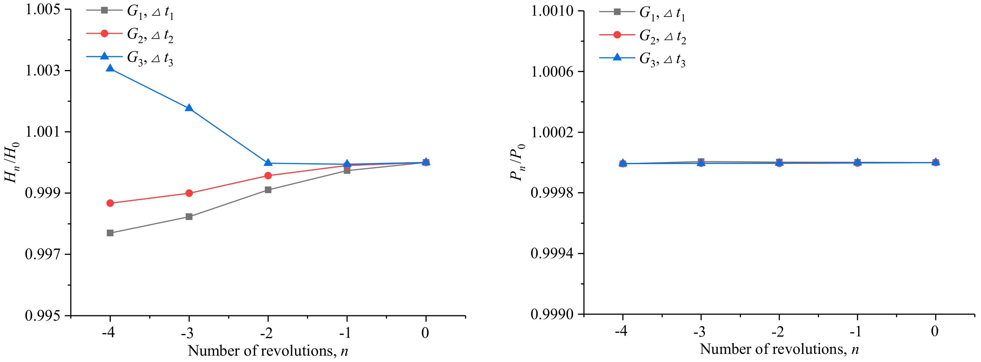
Apart from the residuals, the head and power averaged over a complete revolution of the rotor are used to decide whether the simulation has converged, since the interactions between the rotor and the stator are time-dependent despite the fact that the inflow is uniform. Specifically, the time-averaged head and power of two consecutive revolutions are compared, and when the relative differences are less than 0.1%, results of the last revolution are taken as the final solution. Figure 9 shows the convergence history of the head H and the power P for Q = 0.42 m3/s as an example. The heads differ by less than 0.05% in the last two revolutions for the three solutions, but speed of convergence is much lower than that of the power.
Table 3 shows a comparison of the simulation results and the experimental data [25]. The head and power are mostly under-predicted, and the comparison error ranges between −3.5% and −0.6% for the head and −6.0% and 0.2% for the power.
The iteration uncertainty is evaluated by (3) according to the time-domain results in the last revolution of the rotor. Note that, due to the interactions between the rotor and the stator, the simulated unsteady head and power contain the components at a number of frequencies. The interaction components should be removed when evaluating the iteration uncertainty. According to the relation given by Strasberg et al. [26] for contra-rotating propellers, the interaction components exist at the following frequencies:
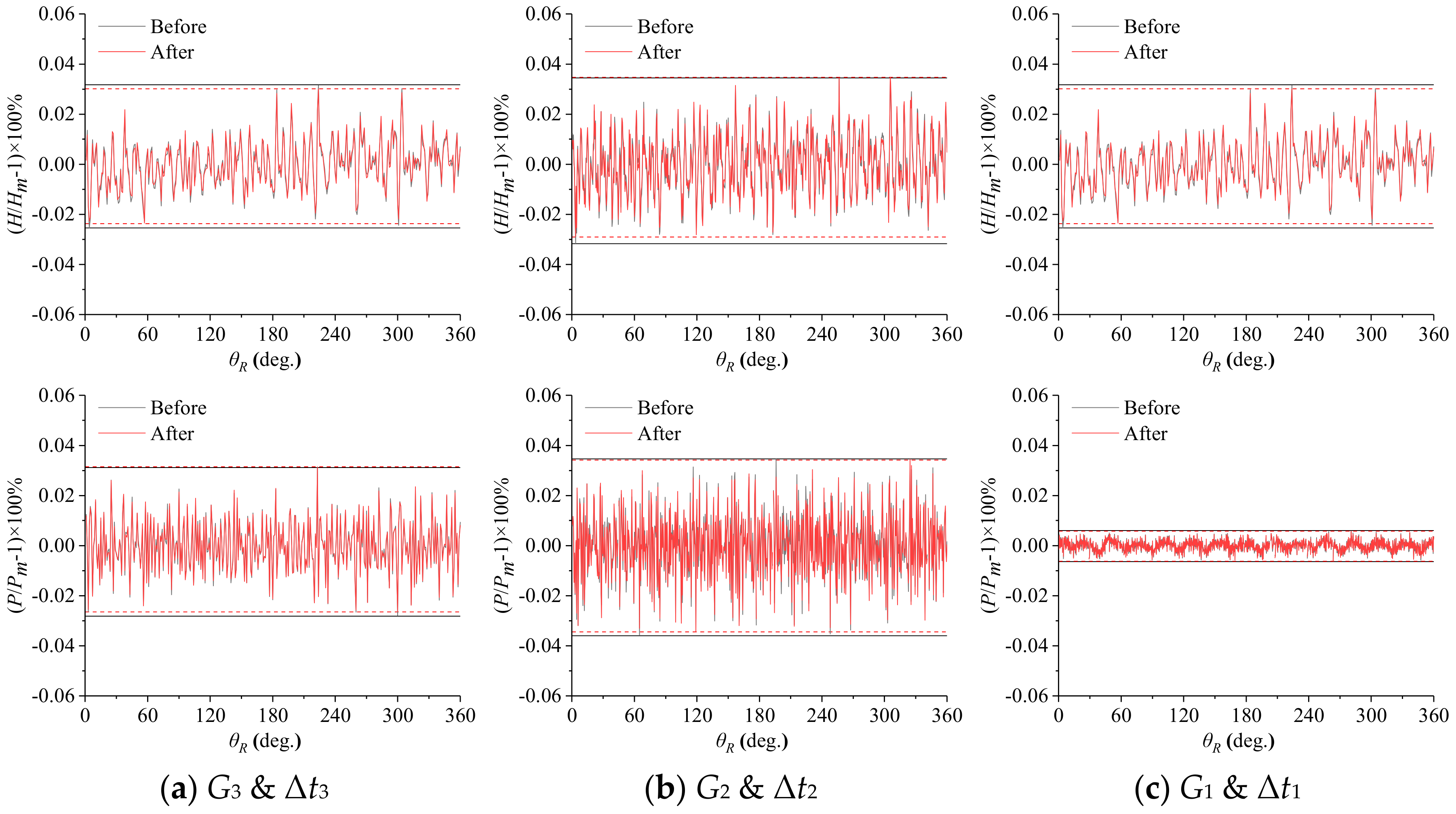
where kZR = mZS, k and m are positive integers; ZR and ZS are blade numbers of the rotor and the stator, respectively; N is the rotational speed (shaft frequency) of the rotor. For the axial-flow pump considered here, ZR = 7, ZS = 9, the lowest frequency of the interaction components is 63 times the shaft frequency. To remove the interaction components, Fourier analyses are performed for the simulated unsteady head and power first; then, the amplitudes at the interaction frequencies are set to zero and the time series are reconstructed. Figure 10 shows a comparison of the time series before and after removing the interaction components. For the combination of rotor and stator blade numbers considered here, the interaction components have little influence on the simulated total fluctuations.
The reconstructed time-series are then used to estimate the iteration uncertainties. Table 4 shows the results, where S denotes the simulation results as listed in Table 3.
Table 5 shows the analysis results for UGT, the uncertainties due to grid and time-step sizes. The following can be observed:
- (1)
- The convergence ratio is 0 < R < 1, which indicates the simulation results converge monotonically when the discretization in time and space is refined simultaneously and consistently. This result justifies the use of the generalized Richardson extrapolation (RE) for evaluating the observed order of accuracy p and the estimated error .
- (2)
- The estimated limiting order of accuracy pest is set to 2, since the governing equations are discretized with second-order schemes in space, and although a first-order scheme is used for the discretization in time.
- (3)
- The correction factor C is sufficiently far from 1 in most cases. Therefore, only the uncertainty UGT is evaluated to give a boundary of the simulation error.
- (4)
- (5)
- The numerical uncertainties are less than 4.3%; and the uncertainties in simulated head are higher than those in simulated power, especially at the low are high flow rates.
4.2. Validation
The absolute value of comparison error |E| is evaluated according to the experimental data D [25] and the simulation results S based on the fine grid G1 and fine time step size Δt1. The validation uncertainty UV is calculated according to (11). Due to the lack of experimental uncertainty data, the experimental uncertainty UD is assumed to be 0.8% by summing up the system accuracies in measuring the flow rate Q, the pressure difference pd − pu, and the torque M, etc. The results in Table 6 indicate that
- (1)
- The validation is successfully achieved at the UV level of 1–4%, except for the power P at Q = 0.35 m3/s and Q = 0.471 m3/s.
- (2)
- For the power P at Q = 0.471 m3/s, the validation is successful at the |E| level of 1%, although the comparison error is larger than the validation uncertainty.
- (3)
- For the power P at Q = 0.35 m3/s, the comparison error is much larger than the validation uncertainty, which indicates that the modeling error is large, and the validation is not achieved.
- (4)
- In most cases investigated here, the principal source of error is unidentifiable since the comparison errors are quite close to the validation uncertainties.
5. Simulated Flow Features
In this section, a detailed investigation is carried out for simulated flow features around rotor blade tips and between the stator and rotor blade rows based on the simulation results with fine grids G1 at the flow rate Q = 0.42 m3/s.
5.1. Tip Clearance Flow
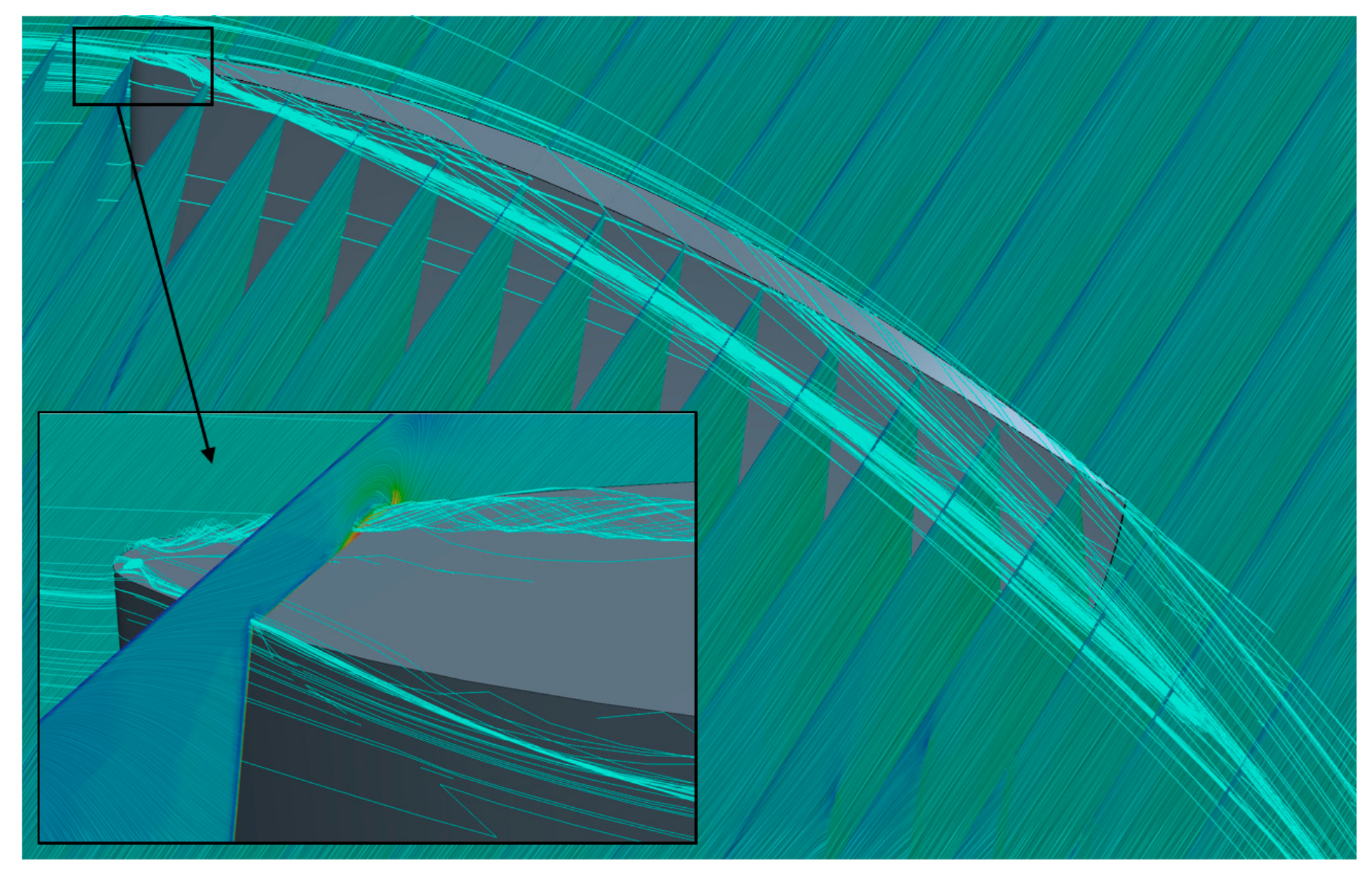
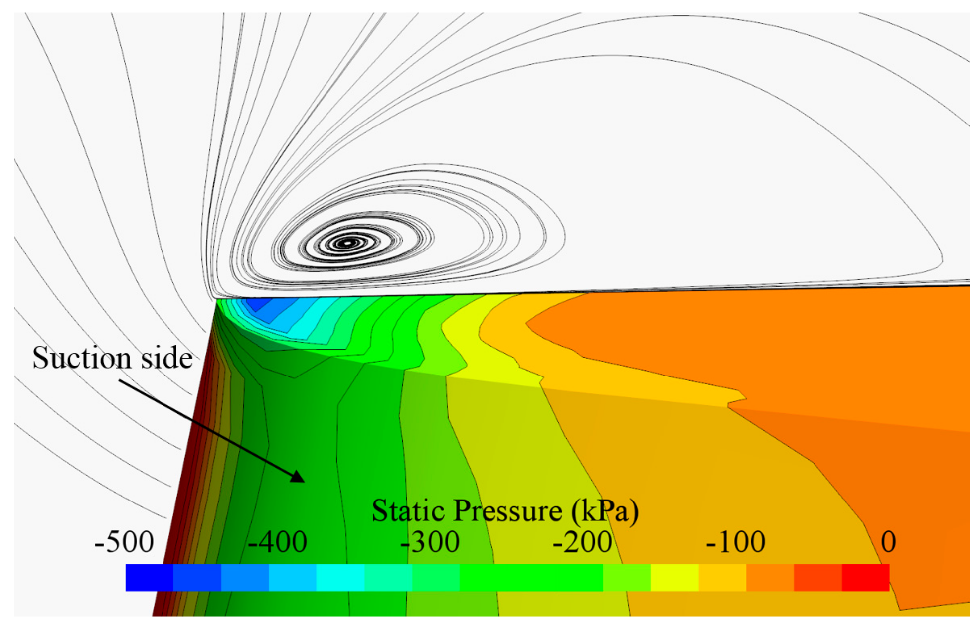
The tip clearance flow is an important factor that influences the cavitation performance of the rotor. Figure 11 shows the streamlines around a blade tip. The flow separates at locations near the leading edge, travels downstream towards the suction side of the blade, and merges together to form the leakage vortices. The flow separation is relatively small at other locations of the tip section. In Figure 12 it is shown that a vortex forms at the leading edge and detaches from the tip surface due to the strong adverse pressure gradients close to the leading edge.
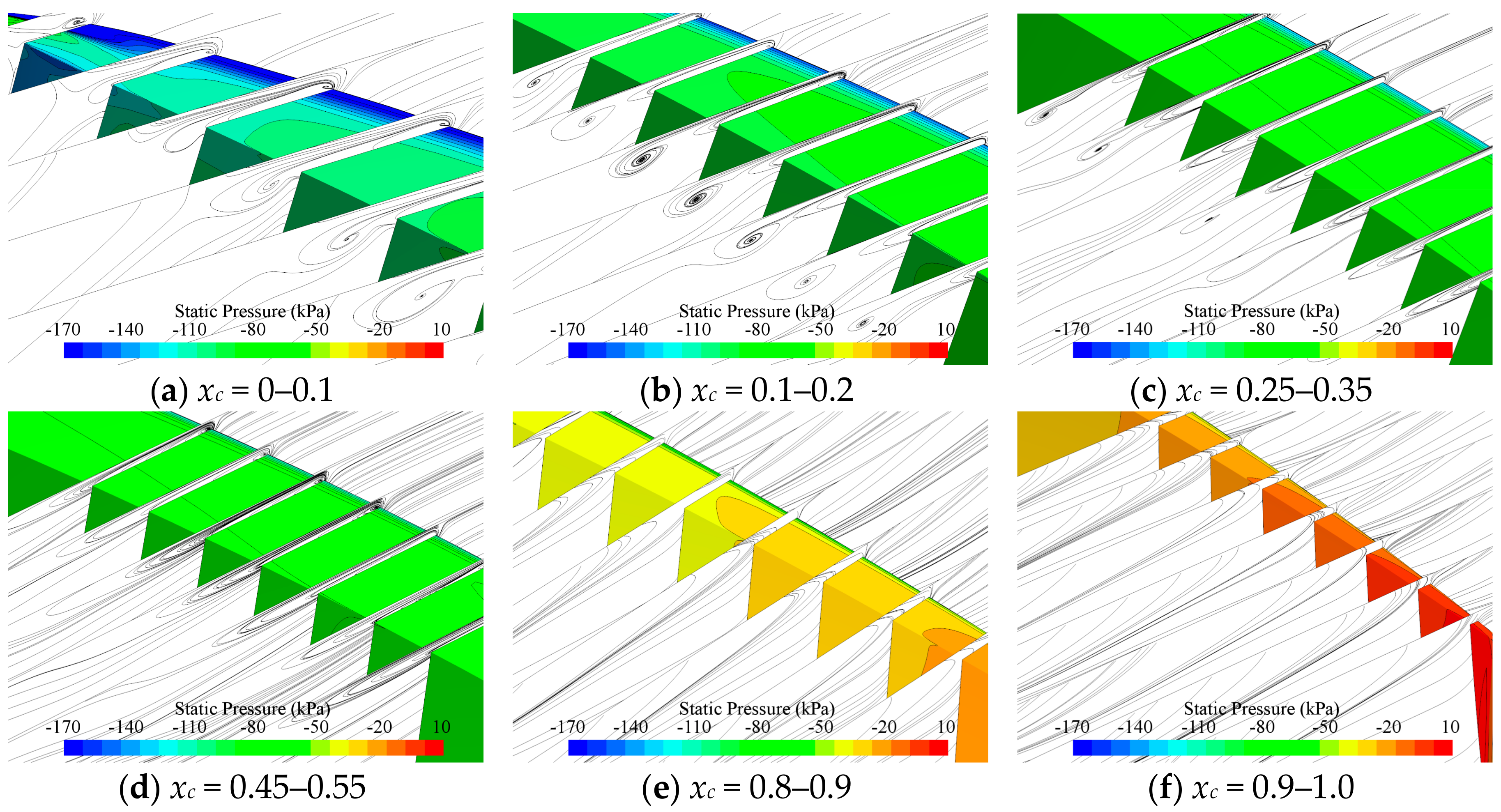
Figure 13 shows in more detail the streamlines in sections across the tip surface. In Figure 13a–c, it is clearly seen that the secondary flow from the pressure side to the suction side of the tip drives the vortical flow that detaches from the vicinity of the leading edge to move towards the suction side as it travels downstream. Meanwhile, the secondary leakage vortices are formed by the separated vortices from the pressure-side corner of the tip at other chordwise locations and travel downstream towards the pressure side of the tip just like the main leakage vortices. The phenomenon of flow separation is evident in the area where there is a large pressure difference between the pressure and suction sides and attenuates gradually behind the mid-chord. The main and secondary leakage vortices may merge at the mid-chord. Finally, they merge near the trailing edge to form a strong vortex. Unlike the open propellers, the tip leakage vortices contract little as they travel downstream.
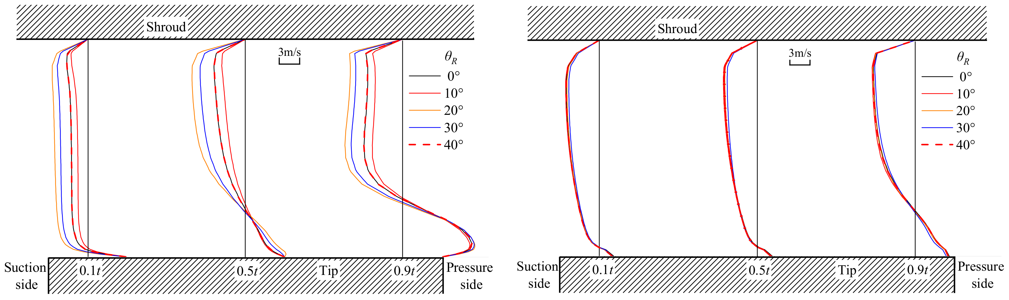
Figure 14 shows the in-plane velocity profiles in the tip clearance, at 10% and 50% chord length. Close to the tip surface, there is a jet-like flow due to the rotation of the blade, which becomes stronger as it goes from the suction side to the pressure side. Over the major part of the tip clearance, the cross flow is clearly driven by the pressure difference between the pressure and the suction sides, although it slows down due to the boundary layer on the shroud surface. Such features are generally similar at the two chordwise locations investigated. However, in the vicinity of the leading edge, the cross flow oscillates at a period of 40 degrees, which is just the angular spacing between adjacent blades of the stator, but becomes almost steady at the mid-chord. The oscillation is probably due to the impingement of the vortices shed from the pre-swirl stator blades.
5.2. Interactions between Rotor and Stator Blades
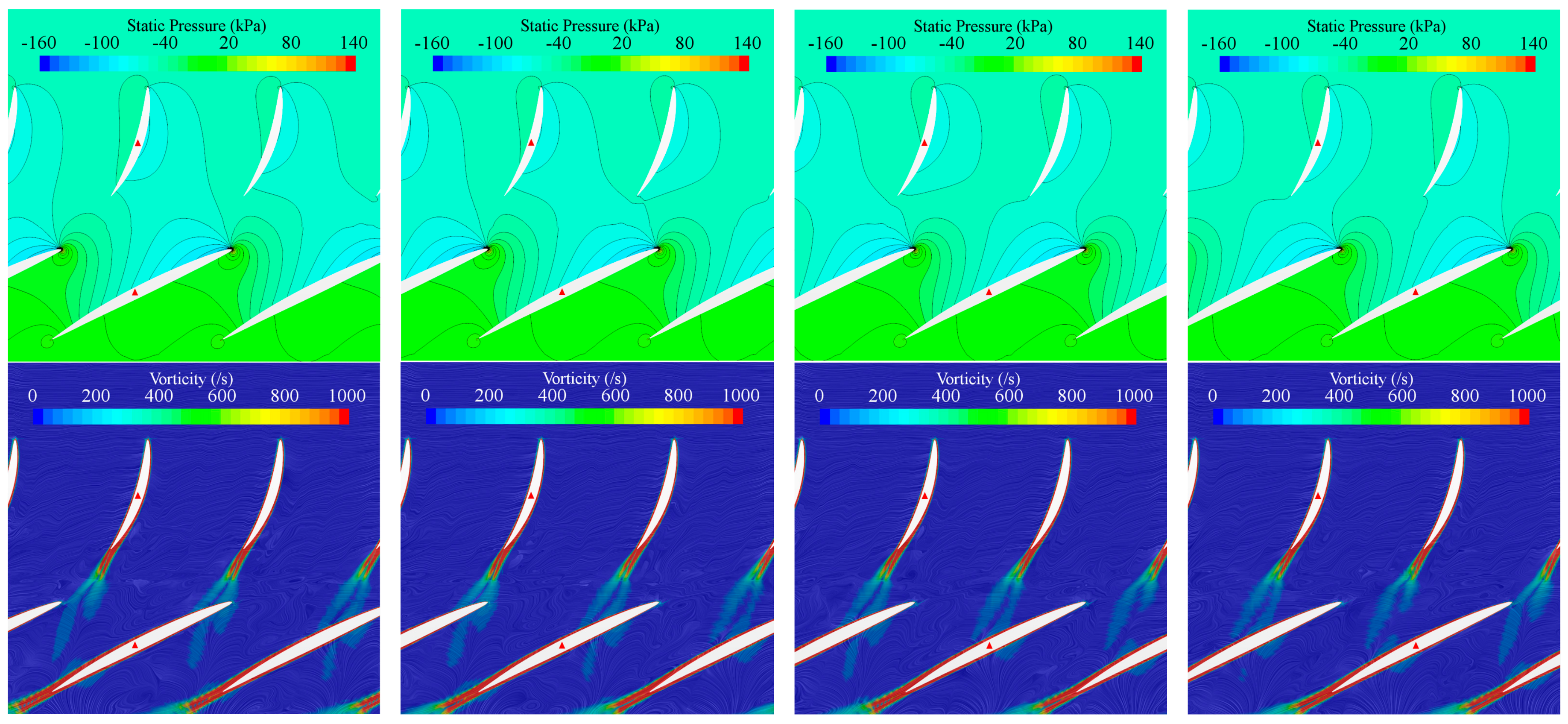
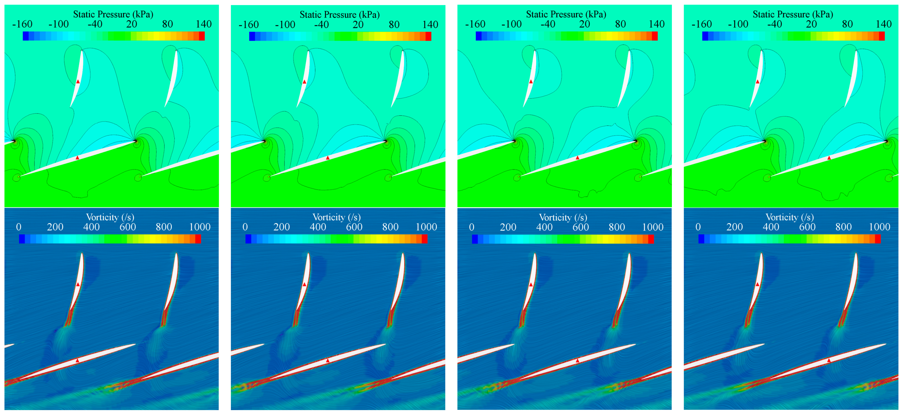
Figure 15 and Figure 16 show the pressure and vorticity contours at typical time instants when the rotor blades sweep across adjacent stator blades. From the variations in the pressure contours around rotor blade sections, it is inferred that the angle of attack changes periodically due to the impingement of shed vortices from stator blades. Meanwhile, the rotor blades counter-act upon the stator blades by changing the pressures on the latter periodically, especially in the downstream part of blade sections. Due to the sliding interfaces between stator and rotor blade rows, the shed vortices behind stator blade sections dissipate abruptly when entering the rotor zone, which is clearly non-physical. It is not impossible to alleviate the grid dissipation by densifying the grids in between the upstream interface and the leading edges of rotor blades, but it would be very expensive computationally.
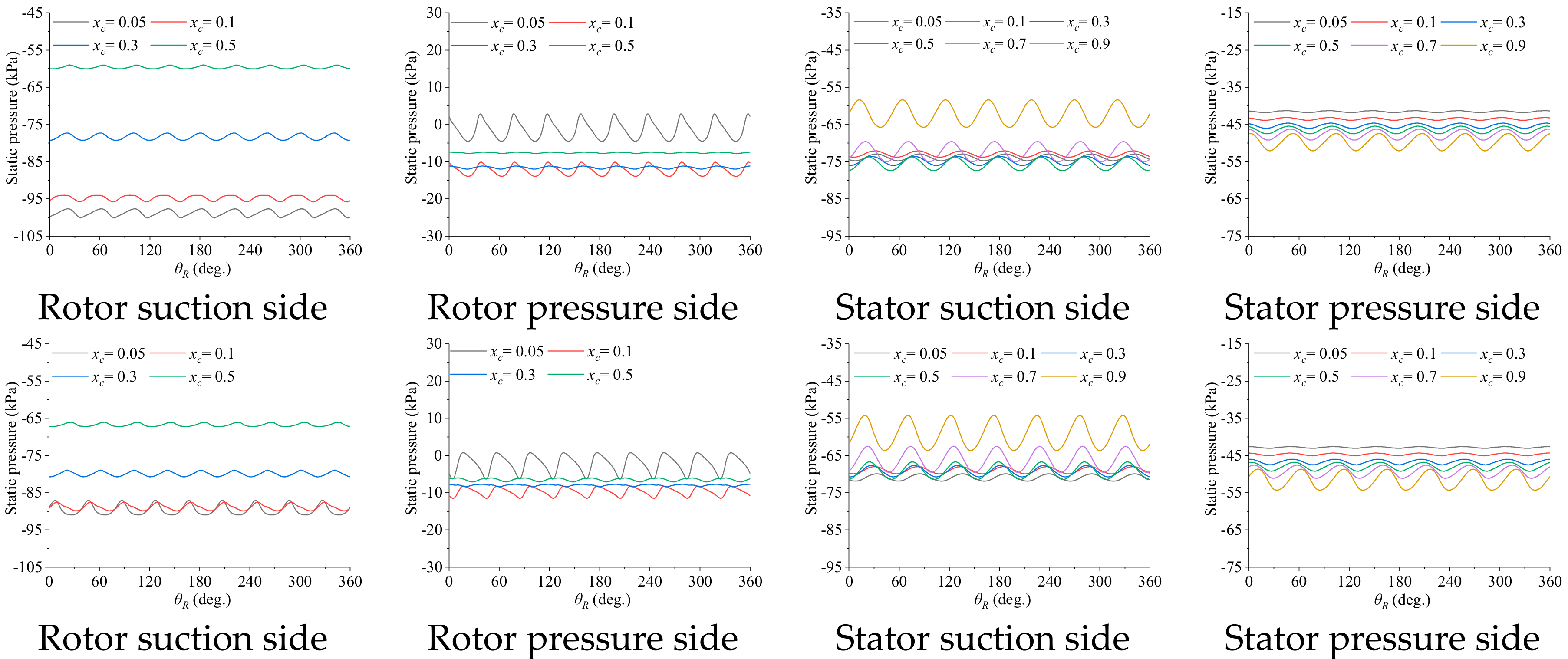
To investigate the rotor/stator interactions quantitatively, the oscillating pressures on rotor and stator blade sections are shown in Figure 17 at 0.7Rtip and 0.95Rtip. The pressures on a rotor blade oscillate nine periods when the rotor completes a revolution, because the rotor blade sweeps across all the nine blades of the stator. For the same reason, the pressures on a stator blade oscillate seven periods since the rotor is seven-bladed. The oscillation amplitudes at the two radii shown in Figure 17 are quite close to each other, for both the rotor and the stator.
On rotor blades, the pressure oscillations are strong close to the leading edge due to the impingement of the vortices shed from the stator but attenuate towards the trailing edge. The oscillations on the pressure side are stronger than those on the suction side. On stator blades, however, the pressure oscillations are strong close to the trailing edge but attenuate towards the leading edge. Apparently, this is due to the counter-action from the rotor blades downstream. Besides, the oscillation amplitudes on the suction and pressure sides are close to each other.
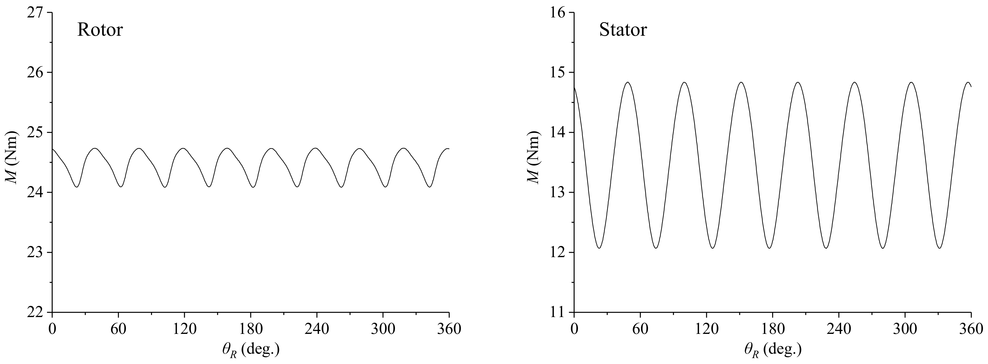
Figure 18 shows the unsteady torques of a rotor blade and a stator blade, respectively. The amplitude of torque oscillations on the stator blade is about three times larger than that on the rotor blade. As shown in Figure 17, the oscillating pressures on the suction and pressure sides of the rotor blade are almost out of phase, but those of the stator blade are more or less in phase. This is the reason why the resultant torque oscillations on a rotor blade are weaker. It is noted that, for either the rotor or the stator, the oscillations in the total force of all the blades are much weaker than that of one blade (see Figure 10), and they only occur at the frequencies subject to the theoretical relation (13) when the inflow is uniform or axisymmetrical.
6. Concluding Remarks
In this work, unsteady RANS simulations of an axial-flow pump for waterjet propulsion are carried out and the numerical simulation uncertainties are analyzed. Unlike the ITTC procedure, the grid uncertainty UG and time step uncertainty UT are replaced by UGT, the numerical uncertainty when grid and time-step sizes are refined simultaneously and consistently. For complex three-dimensional flow problems, the parameter refinement ratios need to be chosen appropriately so that the number of grids is not excessively large, and the time-step size is not too small. However, by doing so, it is almost impossible for the solutions to reach the asymptotic range. The analysis results indicate that the numerical uncertainties in present simulations are less than 4.3%. The validation is successfully achieved in most cases, except for the power at the lowest flow rate considered due to large modeling errors. For the flow rates considered, it is impossible to identify the principal source of error because the comparison errors are quite close to the validation uncertainties. So far as the head and power are concerned, it seems that the present simulation method based on block-structured grids works well from a practical point of view. However, from an uncertainty point of view, the grid and time-step sizes are still not small enough although further refinement would be very challenging computationally and even impractical.
Based on the simulation data using fine grids, the flows in tip-clearance and between rotor and stator blades are investigated. The formation and evolution of the tip leakage vortex is shown by visualizing the flow in the transverse sections along the chord of the tip section. The interactions between rotor and stator blades result in oscillating pressures on each blade of the rotor and the stator. But the oscillations are possibly under-predicted since the vortices shed from stator blades are dissipated artificially when entering the rotor zone.
The simulation method can be improved in two aspects at least. One is to use a second-order scheme for temporal discretization, the other is to reduce the artificial dissipation of the vorticity shed from stator blades due to insufficient grid density in the rotor zone. The latter seems, again, to be quite challenging.
Author Contributions
The numerical computation and analysis were done by J.-T.Q. and X.-Q.D.; C.-J.Y., W.L., and F.N. contributed to the simulation and analysis methodology, as well as composition of the manuscript; Z.-L.W. provided the model test data and discussions about the test setup and measuring methods.
Acknowledgments
The present work was funded by the Waterjet Propulsion Laboratory of Marine Design and Research Institute of China (MARIC) under project No. 61422230103162223005.
Conflicts of Interest
The authors declare no conflicts of interest.
References
- Oberkampf, W.L.; Sindir, M.; Conlisk, A.T. Guide for the Verification and Validation of Computational Fluid Dynamics Simulations; Report No. AIAA G-077-1998; American Institute of Aeronautics and Astronautics: Reston, VA, USA, 1998. [Google Scholar]
- Roache, P.J. Verification and Validation in Computational Science and Engineering; Hermosa: Albuquerque, NM, USA, 1998. [Google Scholar]
- Roache, P.J. Verification of codes and calculations. AIAA J. 1998, 36, 696–702. [Google Scholar] [CrossRef]
- ITTC. Uncertainty analysis in CFD, uncertainty assessment methodology. ITTC-Quality Manual, 4.9-04-01-01. In Proceedings of the International Towing Tank Conference, Shanghai, China, 5–11 September 1999. [Google Scholar]
- ITTC. Uncertainty Analysis in CFD, Guidelines for RANS Codes. ITTC–Recommended Procedures and Guidelines, 7.5-03-01-02. In Proceedings of the International Towing Tank Conference, Seoul, Korea; Shanghai, China, 5–11 September 1999. [Google Scholar]
- Stern, F.; Wilson, R.V.; Coleman, H.W.; Paterson, E.G. Verification and Validation of CFD Simulations; Report No. 407; Iowa Institute of Hydraulic Research: Iowa City, IA, USA, 1999. [Google Scholar]
- Coleman, H.W.; Stern, F. Uncertainties and CFD Code Validation. J. Fluids Eng. 1997, 119, 795–803. [Google Scholar] [CrossRef]
- Richardson, L.F. The approximate arithmetical solution by finite differences of physical problems involving differential equations, with an application to the stresses in a masonry dam. J. Philos. Trans. R. Soc. Lond. Ser. A 1911, 210, 307–357. [Google Scholar] [CrossRef]
- ITTC. Uncertainty analysis in CFD, uncertainty assessment methodology and Procedures. ITTC-Quality Manual, 7.5-03-01-01. In Proceedings of the International Towing Tank Conference, Venice, Italy, 8–14 September 2002. [Google Scholar]
- ITTC. Uncertainty Analysis in CFD, Verification and Validation Methodology and Procedures. ITTC-Recommended Procedures and Guidelines, 7.5-03-01-01. In Proceedings of the International Towing Tank Conference, Wuxi, China, 18 September 2017. [Google Scholar]
- Eça, L.; Vaz, G.; Hoekstra, M. Code verification, solution verification and validation in RANS solvers. In Proceedings of the ASME 2010 29th International Conference on Ocean, Offshore and Arctic Engineering, Shanghai, China, 6–11 June 2010; pp. 597–605. [Google Scholar]
- Larsson, L.; Stern, F.; Visonneau, M. Numerical Ship Hydrodynamics: An Assessment of the 6th Gothenburg 2010 Workshop; Springer Science and Business Media: Berlin, Germany, 2013. [Google Scholar]
- Shen, H.C.; Yao, Z.Q.; Wu, B.S.; Zhang, N.; Yang, R.Y. A new method on uncertainty analysis and assessment in ship CFD. J. Ship Mech. 2010, 14, 1071–1083. [Google Scholar]
- Simonsen, C.D.; Stern, F. Verification and validation of RANS maneuvering simulation of Esso Osaka: Effects of drift and rudder angle on forces and moments. J. Comput. Fluids 2003, 32, 1325–1356. [Google Scholar] [CrossRef]
- Stern, F.; Wilson, R.V.; Coleman, H.; Paterson, E. Comprehensive approach to verification and validation of CFD simulations—Part 1: Methodology and procedures. J. Fluids Eng. 2001, 123, 793–802. [Google Scholar] [CrossRef]
- Zhang, Z.R.; Zhao, F.; Wu, C.S. Research on uncertainty analysis of SUBOFF viscous flow field CFD simulation. In Proceedings of the 2007 Ship Mechanics Conference, Beijing, China, 30 July–1 August 2007. [Google Scholar]
- Yang, Y.R.; Shen, H.C.; Yao, H.Z. Uncertain analysis of CFD simulation on the open-water performance of the propeller. J. Ship Mech. 2010, 14, 472–480. [Google Scholar]
- Rosetti, G.F.; Vaz, G.; Fujarra, A.L.C. URANS calculations for smooth circular cylinder flow in a wide range of Reynolds numbers: Solution verification and validation. J. Fluids Eng. 2012, 134, 121103. [Google Scholar] [CrossRef]
- Diskin, B.; Schwöppe, A. Grid-convergence of Reynolds-Averaged Navier–Stokes solutions for benchmark flows in two dimensions. AIAA J. 2016, 54, 2563–2588. [Google Scholar] [CrossRef]
- Oberkampf, W.L.; Blottner, F.G. Issues in computational fluid dynamics code verification and validation. AIAA J. 1998, 36, 209–272. [Google Scholar] [CrossRef]
- Wilson, R.; Shao, J.; Stern, F. Discussion: Criticisms of the “Correction Factor” Verification Method 1. J. Fluids Eng. 2004, 126, 704–706. [Google Scholar] [CrossRef]
- Rodi, W. Experience with two-layer models combining the k-epsilon model with a one-equation model near the wall. In Proceedings of the 29th Aerospace Sciences Meeting, Reno, Nevada, 7–10 January 1991. [Google Scholar]
- Shih, T.H.; Liou, W.W.; Shabbir, A.; Yang, Z.; Zhu, J. A new k-ε eddy viscosity model for high Reynolds number turbulent flows-model development and validation. Comput. Fluids 1995, 24, 227–238. [Google Scholar] [CrossRef]
- Eça, L.; Hoekstra, M. Code verification of unsteady flow solvers with method of manufactured solutions. In Proceedings of the Seventeenth International Offshore and Polar Engineering Conference. International Society of Offshore and Polar Engineers, Lisbon, Portugal, 1–6 July 2007. [Google Scholar]
- Wang, Z.L. Measurement of the Hydraulic Performance of Axial-Flow Pump Model No.1413; Report No. SM-2016-024; Marine Design and Research Institute of China: Shanghai, China, 2016. [Google Scholar]
- Strasberg, M.; Breslin, J.P. Frequencies of the alternating forces due to interactions of contrarotating propellers. J. Hydronaut. 1976, 10, 62–64. [Google Scholar] [CrossRef]
Figure 1.
The geometric model of the seven-bladed rotor and the nine-bladed pre-swirl stator. The stator blades are connected to the shroud surface without clearance. The shroud surface is omitted.
Figure 1.
The geometric model of the seven-bladed rotor and the nine-bladed pre-swirl stator. The stator blades are connected to the shroud surface without clearance. The shroud surface is omitted.

Figure 2.
The computational domain for the axial-flow pump. The domain is a circular cylinder bounded by the shroud surface, 16 times the shroud diameter in length. The rotor is located at the longitudinal center of the domain, while the stator is located upstream of the rotor.
Figure 2.
The computational domain for the axial-flow pump. The domain is a circular cylinder bounded by the shroud surface, 16 times the shroud diameter in length. The rotor is located at the longitudinal center of the domain, while the stator is located upstream of the rotor.

Figure 3.
Grid topology around rotor blade sections.

Figure 4.
The grid structure in the tip clearance of a rotor. The sections perpendicular to the nose-tail chord of the tip are shown at 10% (top), 50% (middle), and 90% (bottom) chord length.
Figure 4.
The grid structure in the tip clearance of a rotor. The sections perpendicular to the nose-tail chord of the tip are shown at 10% (top), 50% (middle), and 90% (bottom) chord length.

Figure 5.
The surface grids for rotor and stator blades.

Figure 6.
Simulated axial velocity profiles in shroud-surface boundary layer, where h is the normal distance from the shroud surface, X0 is the distance measured from the inlet, and XS is the distance to the nose of shaft cap.
Figure 6.
Simulated axial velocity profiles in shroud-surface boundary layer, where h is the normal distance from the shroud surface, X0 is the distance measured from the inlet, and XS is the distance to the nose of shaft cap.

Figure 7.
Limiting streamlines on rotor (top row) and stator (bottom row) blade surfaces, Q = 0.42 m3/s.
Figure 7.
Limiting streamlines on rotor (top row) and stator (bottom row) blade surfaces, Q = 0.42 m3/s.

Figure 8.
Example of residuals in the last few time steps before convergence, Q = 0.42 m3/s.

Figure 9.
The convergence history of the averaged head H (left) and power P (right) in the last five revolutions before convergence, Q = 0.42 m3/s. The abscissa, n, denotes the number of revolutions relative to the last revolution (n = 0). The ordinates Hn and Pn denote the head and power of the nth revolution, respectively.

Figure 10.
Comparison of the unsteady head H (top row) and power P (bottom row) before (black lines) and after (red lines) removing the components arising from stator/rotor interaction. The abscissa, θR, denotes the angular position of a rotor blade. The head and power are expressed respectively in percents relative to Hm and Pm, the averages over a complete revolution. Q = 0.42 m3/s.

Figure 11.
The streamlines around a blade tip. Q = 0.42 m3/s.

Figure 12.
Pressure contours on the tip surface and streamlines in the tip clearance. Q = 0.42 m3/s.
Figure 12.
Pressure contours on the tip surface and streamlines in the tip clearance. Q = 0.42 m3/s.

Figure 13.
The streamlines (colored by static pressures) in sections across the tip surface, where xc is the chordwise distance from the leading edge in fractions of the chord length. Q = 0.42 m3/s.
Figure 13.
The streamlines (colored by static pressures) in sections across the tip surface, where xc is the chordwise distance from the leading edge in fractions of the chord length. Q = 0.42 m3/s.

Figure 14.
In-plane absolute velocity profiles in the tip clearance at 10% (left) and 50% (right) chord length. The velocity profiles shown at five instantaneous positions of the rotor θR cover the angular spacing between adjacent stator blades. From suction side to pressure side, three sections are taken at 10%, 50% and 90% of the local thickness t, respectively. The velocity magnitude is zero at the vertical straight lines. The shroud is stationary. The rotor tip rotates from left to right. Q = 0.42 m3/s.

Figure 15.
The pressure (top row) and vorticity (bottom row) around stator and rotor blade sections at 0.7Rtip. The rotor blade angle θR = 0°, 10°, 20°, 30° (from left to right). Q = 0.42 m3/s.
Figure 15.
The pressure (top row) and vorticity (bottom row) around stator and rotor blade sections at 0.7Rtip. The rotor blade angle θR = 0°, 10°, 20°, 30° (from left to right). Q = 0.42 m3/s.

Figure 16.
The pressure (top row) and vorticity (bottom row) around stator and rotor blade sections at 0.95Rtip. The rotor blade angle θR = 0°, 10°, 20°, 30° (from left to right). Q = 0.42 m3/s.
Figure 16.
The pressure (top row) and vorticity (bottom row) around stator and rotor blade sections at 0.95Rtip. The rotor blade angle θR = 0°, 10°, 20°, 30° (from left to right). Q = 0.42 m3/s.

Figure 17.
Blade-surface pressure oscillations in a complete revolution of the rotor at 0.7Rtip (top row) and 0.95Rtip (bottom row). xc denotes the chordwise location from section nose in fractions of the chord length. θR denotes the angular position of a rotor blade. Q = 0.42 m3/s.
Figure 17.
Blade-surface pressure oscillations in a complete revolution of the rotor at 0.7Rtip (top row) and 0.95Rtip (bottom row). xc denotes the chordwise location from section nose in fractions of the chord length. θR denotes the angular position of a rotor blade. Q = 0.42 m3/s.

Figure 18.
Oscillations of the torques on a rotor blade (left) and a stator blade (right). θR denotes the angular position of the rotor blade. Q = 0.42 m3/s.
Figure 18.
Oscillations of the torques on a rotor blade (left) and a stator blade (right). θR denotes the angular position of the rotor blade. Q = 0.42 m3/s.


Table 1.
Key parameters of the computational grids.
| Grid ID | Maximum Cell Size on Blade Surface (mm) | First-Layer Cell Height from Blade Surface (mm) | Number of Cells in Tip-Clearance | Total Number of Cells (Million) | |||
|---|---|---|---|---|---|---|---|
| Stator | Rotor | Stator | Rotor | Radial | Circumferential | ||
| G3 | 5 | 4 | 0.02 | 0.01 | 10 | 16 | 1.79 |
| G2 | 3.54 | 2.83 | 0.014 | 0.007 | 15 | 22 | 4.87 |
| G1 | 2.5 | 2 | 0.01 | 0.005 | 20 | 30 | 13.17 |
Table 2.
Range of the surface-averaged y+, Q = 0.35 m3/s–0.471 m3/s.
| Grid ID | Stator | Rotor | Tip Clearance |
|---|---|---|---|
| G3 | 3.2–4.2 | 1.9–2.3 | 5.7–5.8 |
| G2 | 2.3–3.0 | 1.4–1.6 | 4.7–4.8 |
| G1 | 1.7–2.3 | 1.0–1.3 | 3.3–3.4 |
Table 3.
Comparison of simulation results and experimental data [25] for the axial-flow pump.
Table 3.
Comparison of simulation results and experimental data [25] for the axial-flow pump.
| Q (m3/s) | Grid, Time-Step Size | Simulation Result S | Experimental Data D | Comparison Error E (%D) | |||
|---|---|---|---|---|---|---|---|
| H (m) | P(kW) | H (m) | P (kW) | H | P | ||
| 0.35 | G3, Δt3 | 7.320 | 29.473 | 7.450 | 31.341 | −1.47 | −5.96 |
| G2, Δt2 | 7.373 | 29.541 | −1.04 | −5.74 | |||
| G1, Δt1 | 7.406 | 29.584 | −0.59 | −5.61 | |||
| 0.42 | G3, Δt3 | 5.221 | 25.343 | 5.400 | 25.957 | −3.31 | −2.36 |
| G2, Δt2 | 5.247 | 25.414 | −2.83 | −2.09 | |||
| G1, Δt1 | 5.267 | 25.473 | −2.45 | −1.87 | |||
| 0.471 | G3, Δt3 | 3.476 | 20.341 | 3.600 | 20.305 | −3.44 | 0.18 |
| G2, Δt2 | 3.521 | 20.456 | −2.18 | 0.75 | |||
| G1, Δt1 | 3.546 | 20.513 | −1.49 | 1.02 | |||
Table 4.
Iteration uncertainties in the simulations.
| Q (m3/s) | G3, Δt3 (%S) | G2, Δt2 (%S) | G1, Δt1 (%S) | |
|---|---|---|---|---|
| 0.35 | H | 0.03 | 0.02 | 0.02 |
| 0.42 | 0.03 | 0.03 | 0.01 | |
| 0.471 | 0.04 | 0.04 | 0.01 | |
| 0.35 | P | 0.03 | 0.02 | 0.01 |
| 0.42 | 0.03 | 0.03 | 0.01 | |
| 0.471 | 0.04 | 0.04 | 0.01 |
Table 5.
Results of the numerical uncertainties at different flow rates.
| Q (m3/s) | ε21 | ε32 | R | p | C | UGT | USN (%S) | ||
|---|---|---|---|---|---|---|---|---|---|
| 0.35 | H | −0.033 | −0.053 | 0.642 | 1.280 | −0.060 | 0.558 | 0.113 | 1.52 |
| 0.42 | −0.021 | −0.025 | 0.814 | 0.593 | −0.091 | 0.228 | 0.231 | 4.27 | |
| 0.471 | −0.025 | −0.045 | 0.564 | 1.651 | −0.033 | 0.772 | 0.048 | 1.33 | |
| 0.35 | P | −0.043 | −0.068 | 0.625 | 1.355 | −0.071 | 0.599 | 0.129 | 0.41 |
| 0.42 | −0.059 | −0.071 | 0.836 | 0.516 | −0.302 | 0.196 | 0.787 | 3.03 | |
| 0.471 | −0.057 | −0.115 | 0.496 | 2.025 | −0.056 | 1.017 | 0.062 | 0.30 |
Table 6.
The comparison error |E| and validation uncertainty UV at different flow rates.
| Q (m3/s) | |E| (%D) | UV (%D) | ||
|---|---|---|---|---|
| H | P | H | P | |
| 0.35 | 0.59 | 5.61 | 1.72 | 0.90 |
| 0.42 | 2.46 | 1.86 | 4.35 | 3.14 |
| 0.471 | 1.50 | 1.02 | 1.55 | 0.86 |
© 2018 by the authors. Licensee MDPI, Basel, Switzerland. This article is an open access article distributed under the terms and conditions of the Creative Commons Attribution (CC BY) license (http://creativecommons.org/licenses/by/4.0/).
Share and Cite
MDPI and ACS Style
Qiu, J.-T.; Yang, C.-J.; Dong, X.-Q.; Wang, Z.-L.; Li, W.; Noblesse, F. Numerical Simulation and Uncertainty Analysis of an Axial-Flow Waterjet Pump. J. Mar. Sci. Eng. 2018, 6, 71. https://doi.org/10.3390/jmse6020071
AMA Style
Qiu J-T, Yang C-J, Dong X-Q, Wang Z-L, Li W, Noblesse F. Numerical Simulation and Uncertainty Analysis of an Axial-Flow Waterjet Pump. Journal of Marine Science and Engineering. 2018; 6(2):71. https://doi.org/10.3390/jmse6020071
Chicago/Turabian StyleQiu, Ji-Tao, Chen-Jun Yang, Xiao-Qian Dong, Zong-Long Wang, Wei Li, and Francis Noblesse. 2018. "Numerical Simulation and Uncertainty Analysis of an Axial-Flow Waterjet Pump" Journal of Marine Science and Engineering 6, no. 2: 71. https://doi.org/10.3390/jmse6020071
Note that from the first issue of 2016, this journal uses article numbers instead of page numbers. See further details here.