Boundary Element Modelling Aspects for the Hydro-Elastic Analysis of Flexible Marine Propellers


Maritime & Transport Technology Department, Delft University of Technology, Mekelweg 2, 2628 CD Delft, The Netherlands
*
Author to whom correspondence should be addressed.
J. Mar. Sci. Eng. 2018, 6(2), 67; https://doi.org/10.3390/jmse6020067
Submission received: 10 April 2018
/
Revised: 30 May 2018
/
Accepted: 1 June 2018
/
Published: 5 June 2018
(This article belongs to the Special Issue Marine Propulsors)
Abstract
:Boundary element methods (BEM) have been used for propeller hydrodynamic calculations since the 1990s. More recently, these methods are being used in combination with finite element methods (FEM) in order to calculate flexible propeller fluid–structure interaction (FSI) response. The main advantage of using BEM for flexible propeller FSI calculations is the relatively low computational demand in comparison with higher fidelity methods. However, the BEM modelling of flexible propellers is not straightforward and requires several important modelling decisions. The consequences of such modelling choices depend significantly on propeller structural behaviour and flow condition. The two dimensionless quantities that characterise structural behaviour and flow condition are the structural frequency ratio (the ratio between the lowest excitation frequency and the fundamental wet blade natural frequency) and the reduced frequency. For both, general expressions have been derived for (flexible) marine propellers. This work shows that these expressions can be effectively used to estimate the dry and wet fundamental blade frequencies and the structural frequency ratio. This last parameter and the reduced frequency of vibrating blade flows is independent of the geometrical blade scale as shown in this work. Regarding the BEM-FEM coupled analyses, it is shown that a quasi-static FEM modelling does not suffice, particularly due to the fluid-added mass and hydrodynamic damping contributions that are not negligible. It is demonstrated that approximating the hydro-elastic blade response by using closed form expressions for the fluid added mass and hydrodynamic damping terms provides reasonable results, since the structural response of flexible propellers is stiffness dominated, meaning that the importance of modelling errors in fluid added mass and hydrodynamic damping is small. Finally, it is shown that the significance of recalculating the hydrodynamic influence coefficients is relatively small. This fact might be utilized, possibly in combination with the use of the closed form expressions for fluid added mass and hydrodynamic damping contributions, to significantly reduce the computation time of flexible propeller FSI calculations.
1. Introduction
Over the last two decades, an increased interest in flexible propellers can be noticed given the growing list of publications on the hydro-elastic analysis of flexible marine propellers. Several publications present a methodology for the numerical analysis of these types of propellers in steady and unsteady inflow conditions. These methods typically involve partitioned fluid–structure interaction (FSI) computations, meaning that the fluid and structural problem are separately solved and coupling iterations are required to converge to the fully coupled solution. For steady propeller FSI computations mainly Reynolds-averaged Navier–Stokes (RANS) methods [1,2,3,4] and boundary element methods (BEM) [5,6,7,8,9,10,11,12] have been used for solving the fluid part of the coupled problem.
The fundamental difference between RANS and BEM is that, in the latter, a potential flow is assumed, meaning that phenomena as flow separation, flow transition, boundary layers and vorticity dynamics are not modelled. Results of validation studies on flexible propellers in open water conditions with BEM-FEM (finite element method) and RANS-FEM methods have been presented in [13]. Despite the limitations of a BEM and the complicated flow characteristics considered in that work, a fairly good estimate of the propeller hydro-elastic response was obtained with the BEM-FEM approach. Given the relatively low computational demand of BEM in comparison to a RANS method, BEM is an attractive method for the FSI analysis of flexible propellers.
The BEM modelling of flexible propellers in steady and unsteady flow requires several modelling choices—for instance, how to include propeller deformations in the BEM analysis. Is a full geometry update necessary at every time step or can an accurate solution be obtained more efficiently by partly updating the propeller geometry every time step? How can fluid added mass and hydrodynamic damping be included: explicitly with closed form expressions [7] or implicitly in the BEM calculation? Answers to these questions do not seem to be available in literature. The main purpose of this work is to fill this knowledge gap and therefore several modelling choices have been evaluated.
The BEM models for steady and unsteady flexible propeller analyses as proposed in this work look similar to the model as presented in [7]. However, on the following aspects, these models are different. In [7], the BEM modelling relies on the assumption of negligible small blade deformations. The most extensive model presented in this work is applicable for large elastic blade deformations, since blade deformation and vibration effects are implicitly included in the BEM calculation by updating the blade geometry and the body boundary impermeability condition at each computation step. Another difference is that the BEM modelling approach as presented in [7] is based on an explicit treatment of fluid added mass and hydrodynamic damping forces, while, in this work, both an implicit and explicit modelling of fluid added mass and hydrodynamic damping effects have been considered.
The consequences of BEM modelling choices depend significantly on flow condition and structural behaviour. The two dimensionless quantities that characterise propeller structural behaviour and flow condition are the structural frequency ratio (the ratio between the lowest excitation frequency and the fundamental wet blade natural frequency) and the reduced frequency. For both, general expressions have been derived for (flexible) marine propellers.
This paper is structured as follows. In Section 2, general expressions for reduced frequencies and structural frequency ratios of flexible composite propellers are derived. Section 3 describes the BEM modelling of flexible propellers. Section 4 presents the derivation of closed form expressions for fluid added mass and hydrodynamic damping. In Section 5, the hydrodynamic loads on a plunging hydrofoil are investigated and important conclusions are drawn with respect to the frequency dependence of fluid added mass and hydrodynamic damping. Section 6 presents different BEM models for steady and unsteady flexible propeller calculations and include the results of a comparative study. Section 7 contains the conclusions.
2. Flow and Structural Response Characterisation
In this section, expressions will be derived to estimate the characteristics of fluid and structural response for flexible marine propellers. Section 2.1 provides expressions for the fundamental blade natural frequency in air and water and the structural frequency ratio. Section 2.2 shows a typical value for the propeller flow reduced frequency. In Section 2.3, estimated natural frequencies in air and water obtained for flexible versions of the highly skewed Seiun–Maru propeller have been compared to FEM calculation results.
2.1. Structural Frequency Ratio
The structural response of a one degree-of-freedom (1DOF) linear mass-spring-damper system can be assigned to one of the following regimes, depending on the ratio between excitation frequency and natural frequency :
- ; quasi-static regime, structural response dominated by stiffness.
- ; resonance regime, structural response dominated by damping.
- ; dynamic regime, structural response dominated by mass.
The fundamental natural frequency of a propeller blade is the frequency of the first bending mode. The blade natural frequencies depend on the stiffness and mass and can be computed using solution techniques available in FEM software. For a quick approximation of the first two natural frequencies in air and water, formulas are provided in [14,15]. The fundamental dry natural frequency, , in rad/s can be estimated for moderately skewed propellers with
where R is the propeller radius, is the hub radius, E the Young’s modulus the blade material density, the mean blade thickness, the root blade thickness, the mean chord length and the root chord length. The fundamental wet natural frequency of nickel aluminium bronze (NAB) propellers is generally 62–64% of the value in air [16], meaning that, for the first mode, the modal fluid added mass is approximately 2.5 times the NAB blade modal mass. Thus, the fundamental wet natural frequency, , for any propeller material is given by
where is the density of the NAB material.
From Equations (1) and (2), it can be concluded that, when NAB blade material with a typical Young’s modulus and density of 110 GPa and 7600 kgm is replaced by a glass–epoxy composite material with a typical Young’s modulus and density of 20 GPa and 1700 kgm, the dry natural frequencies will slightly decrease. When a carbon–epoxy material is considered with a typical Young’s modulus and density of 75 GPa and 1600 kgm, the dry natural frequencies will be significantly higher than for the NAB equivalent. The fundamental wet natural frequency of a glass–epoxy blade will be considerably smaller than its NAB equivalent, while for a carbon–epoxy blade, it is approximately the same. Due to the lower material density of fibre reinforced plastics, the fluid added mass has a more pronounced effect on the wet natural frequencies than in the case of a NAB propeller. From Equations (1) and (2), it can be concluded that the dry and wet blade frequencies scale inversely proportional with the geometrical blade scale.
Analogous to the structural frequency ratio of a 1DOF linear mass-spring-damper system, the structural response behaviour of propeller blades can be characterised by the ratio of the frequency corresponding to the dominant blade mode and the excitation frequency. As will be shown latter on, the response of flexible propellers is stiffness dominated, then, the first blade mode will dominate the structural response. Hence, the wet fundamental blade frequency is the typical frequency used for the structural frequency ratio. The lowest excitation frequency is the shaft rotation frequency. Since the shaft rotation speed, n, is related to the blade radius by the tip speed , the following expression for the ratio between excitation frequency and wet fundamental blade frequency, i.e., the structural frequency ratio, , can be derived
In order to avoid cavitation, a typical value for the maximum allowable tip speed is around 35 m/s. Therefore, the maximum tip speed in ship propeller design is a constant rather than a variable. By proportionally scaling the propeller dimensions R, , , , and , the structural frequency ratio does not change. Hence, the structural frequency ratio is independent of the geometrical propeller scale.
2.2. Propeller Flow Reduced Frequency
For fluids around lifting bodies, a dimensionless number exists that describes the unsteadiness of the flow and is called the reduced frequency. In the expression for the reduced frequency, k, an oscillation frequency is related to the flow speed:
where c is the chord length and the undisturbed flow velocity. For small reduced frequencies, the unsteadiness of the flow is negligible and a quasi-steady approach can be justified. For higher reduced frequencies, the circulatory lift reduces, which is called the lift deficiency and a phase lag between the circulatory part of the lift and the body motion exists due to the wake vorticity. Lift deficiency and phase lag functions for a flat plate foil in small amplitude unsteady motion were derived by Theodorsen [17], see Figure 1.
The propeller flow reduced frequency at 70% of the blade radius is obtained from the shaft rotation speed and is given by
where is the chord length at and is typically 40% of the blade diameter, D. is the undisturbed flow speed at . is approximately . Hence, for conventional propellers, a typical value for the reduced frequency at is . This value can be considered as highly unsteady according to Figure 1 and appears to be independent of the geometrical propeller scale.
2.3. Seiun–Maru Propeller Frequencies
The expressions for the fundamental natural frequencies have been verified by comparing estimated dry and wet fundamental blade frequencies to FEM calculated frequencies for the highly skewed Seiun–Maru propeller. The Seiun–Maru is a Japanese training vessel. The geometry of the propeller is in the public domain [18] and its main particulars are summarized in Table 1.
Figure 2 shows the dry and wet fundamental blade frequencies calculated with the FEM and estimated with Equations (1) and (2). For the various materials, the properties as mentioned before have been used. For the FEM calculations, a Poisson ratio of has been adopted and the fluid added mass has been calculated with the approach described in Section 4. The differences between the frequencies obtained with FEM and the estimation formulas are smaller than 20% for all the cases. It is expected that, for propellers with less skew, the differences will be smaller, since Equation (1) was proposed for moderately skewed propellers [14,15]. Nevertheless, the estimated natural frequencies are accurate enough to identify the structural response regime and Equation (3) is proposed to attribute the structural behaviour to stiffness, damping or mass dominated response. For a maximum allowable tip speed of 35 m/s, the structural frequency ratios as given in Figure 3 have been obtained for the various Seiun–Maru propellers. It can be concluded that the structural response of composite propeller blades is expected to be predominantly quasi-static and probably a quasi-static structural approach might give a good approximation of the blade response. This will be further evaluated in Section 6.
3. Hydrodynamic Method for Propeller Forces
3.1. Potential Flow Theory
In the present study, the BEM PROCAL has been used for the hydrodynamic calculations. PROCAL is a panel method developed by the Maritime Research Institute Netherlands (MARIN) for the Cooperative Research Ships [19,20]. PROCAL solves the integral equation for the velocity potential in a fluid domain based on the Morino formulation [21]. In this integral formulation, the propeller induced velocity disturbances are considered irrotational. Then, by defining the scalar variable as the disturbance velocity potential, the total velocity, , relative to the operating propeller becomes
where t is the time and is the position vector in a Cartesian coordinate system. The undisturbed velocity, , can be written as the sum of the ship’s effective wake field velocity and the effect of the propeller angular velocity, with the wake field velocity, , and with the propeller angular velocity, ,
The flow is assumed to be incompressible and has a constant density. Therefore, Laplace’s equation applies to the disturbance velocity potential,
Then, the fluid pressures p are related to the total velocity and the disturbance velocity potential according to Bernoulli’s law,
For a propeller, is the pressure far upstream (along the shaft axis) and it obeys the hydrostatic law, being the atmospheric pressure at the free surface, and submergence, z, at the shaft as, . In order to solve Equation (8), boundary conditions have to be imposed on the propeller surface () and wake sheet (), which contains the shed vorticity. On the propeller surface, an impermeability condition is imposed,
where is the surface normal. For the wake sheet, a kinematic and dynamic boundary condition can be formulated. The kinematic boundary condition prescribes that the wake sheet is a stream-surface of the flow,
The wake sheet itself is an imaginary surface in the flow with zero thickness. The wake sheet cannot support a pressure difference between its upper and lower side. This dynamic boundary condition can be written as
where and denote the upper and lower side of the wake sheet. At the blade trailing edge, this is the so-called Kutta condition.
3.2. Integral Formulation for Disturbance Potential
A relation between the potential at any point in the fluid domain and the source strengths (normal component of the disturbance velocity at the body boundary) exists and is given by the integral equation following from the third Green’s identity. Using Morino’s formulation [21], this can be written as
where is a point in the fluid domain, and is a point on the fluid domain boundary surface. G is the Green’s function for the Laplace equation defined as
is the outward normal at . is a constant that depends on the field point and is if is on the fluid boundary surface. With the dynamic boundary condition for the wake sheet, the following integral equation is obtained:
In this integral equation, the geometry of the body and wake sheet are constant. This means that the points on the fluid domain boundary surfaces and the surface areas are time invariant, which is obviously not the case for a deformable body. In that case, the integral formulation of Equation (15) transforms to the unsteady flow and time-variant body integral equation,
3.3. Numerical Formulation
The integral equations of Equations (15) and (16) are solved in PROCAL by approximating the surfaces and by number of panels. On each panel, a collocation point is defined where the integral equation is applied. Finally, a system of equations is obtained, unknown in the strengths of the source and dipole elements. With the imposed boundary conditions, the system of equations can be solved and the potential at the boundaries is obtained. This subsection briefly describes and presents the system of equations for the non-cavitating propeller calculations considered in this work. For the formulation of the discretised problems, the discretisation parameters and equations as presented in [19] have been used. For a more thorough derivation, one is referred to that publication.
3.3.1. Geometry Discretisation
In PROCAL, the entire fluid domain boundary surface, consisting of body surface and wake surface , is decomposed in a key part containing one blade with corresponding hub section and wake sheet and a symmetry part including the other blades, hub sections and wake sheets. The motivation for this subdivision in key- and symmetry surfaces is to obtain a smaller system of equations by utilizing the symmetry properties of ship propellers. The symmetry of flexible propellers in an unsteady flow can be questioned due to time varying deformations and will be discussed further in Section 6.
Figure 4 shows the discretised geometry of a propeller and wake. The discretisation parameters displayed in this figure have the following meaning:
- : Number of surfaces, is 2; the blade surfaces and the hub surfaces.
- : Number of symmetries for each surface. In general, is equal to the number of propeller blades.
- : Number of panels in the streamwise direction.
- : Number of panels in the radial direction.
- : Number of panels on the wake sheet in the streamwise direction.
- : Number of panels on the wake sheet in the radial direction.
3.3.2. Steady Flow and Rigid Propeller Formulation
For a rigid propeller in a steady flow, Equation (15) can be discretized as follows:
where , and are the hydrodynamic influence coeficients for the body dipoles, body sources and wake dipoles, respectively. They are defined as
and
and are the source and dipole strengths respectively at collocation point on the body surface. is the dipole strength at collocation point on the wake surface. is the total number of panels for which the flow quantities have to be solved: .
In case of a steady flow calculation, the symmetry surfaces can be taken into account by adding the influence coefficients of key- and symmetry surfaces together; for instance, for the dipole influence coefficients,
In general, the strength of a vortex shed by a lifting body is time invariant. This follows from the dynamic and kinematic boundary condition on the wake surface (Equations (11) and (12)); by using Bernoulli’s theorem, this yields that the dipole strengths are time invariant following a wake particle. Furthermore, for steady flow conditions the dipole strengths on the wake sheet are the same at fixed j but different i. Accordingly, the dipole influence coefficients of each j strip can be added,
Making use of the symmetry properties of the problem and the summation of the wake dipole influence coefficients, Equation (17) can be written as
The body source strengths are known from the impermeability boundary condition (Equation (10)) and moved to the right-hand-side of the equation. The matrix defined at the left-hand-side of Equation (22) is a full square matrix with dimension . However, the number of known source strengths is equal to , meaning that an additional set of number of equations have to be defined in order to close the system of equations. These additional equations can be deduced from the Kutta condition imposing that the tangential velocities at the blade trailing edge, computed on the upper and lower side of the body surface, are equal. The discretised translation of the Kutta condition is the Morino Kutta condition [21] expressing that the difference of the potential values between the upper and lower side of the body trailing edge is equal to the wake dipole strength,
This equation holds for every strip j of the propeller, resulting in a number of additional equations per surface. Then, the system of equations becomes
where , and are the body dipole, wake dipole and body source influence coefficients matrices, respectively. The matrices , and contain only ones and zeros to account for the Morino Kutta condition. Equation (24) can be written as
where is the total dipole influence coefficients matrix.
3.3.3. Unsteady Flow and Rigid Propeller Formulation
For an unsteady flow and rigid propeller, the inflow conditions and, consequently, the source strengths depend on the blade position.
In PROCAL, an unsteady problem is solved by performing k steady flow like calculations, where k is the number of revolutions, , required for convergence times the number of timesteps during one revolution, , i.e., .
There is an important difference between a steady computation and the k-th calculation of an unsteady computation. For steady calculations, the symmetry properties of the propeller inflow and geometry are exploited to obtain a smaller system of equations. In case of an unsteady flow, the inflow is generally non-symmetric. To avoid simultaneously solving the system of equations for all key and symmetry surfaces, an iterative procedure is applied.
In this iterative procedure, the distinction between the key and symmetry surfaces is maintained. The system of equations is solved for the key surfaces only, while, for the symmetry surfaces, a previous solution of the key surfaces is taken from the timestep when the key surfaces were at the same spatial position as the symmetry surfaces at the current timestep. This means that the contribution of the symmetry surfaces can be moved to the right-hand-side of the equation. Then, the solution is obtained by solving the systems of equations every timestep and a multiple number of revolutions until convergence. In this way, the discretised system of equations are given by
3.3.4. Unsteady Flow and Flexible Propeller Formulation
In case of an unsteady flow and flexible propeller, all the influence coefficients are time dependent, which results in
Equation (27) shows that the symmetry influence coefficients are time dependent as well and are equal to the influence coefficients of the symmetry surfaces on the key surfaces at timestep when the key surfaces were at the same spatial position as the symmetry surfaces at the current timestep. This means that the symmetry surface influence coefficients have to be stored in memory times increasing the required computer memory significantly. Therefore, in the BEM model for unsteady flexible propeller calculations, it has been decided to use the symmetry surface influence coefficients at time step k for the symmetry surface influence coefficients of time step . This modelling choice, together with the importance of the recalculation of the key blade influence coefficients, will be discussed further in Section 6.
3.3.5. The Kutta Condition for Flexible Propellers
It has to be discussed whether the Kutta condition can be applied in the unsteady flexible propeller BEM model because the Kutta condition was proposed solely for steady flows [22]. Later, the Kutta condition has been modified for unsteady models, which had been questioned [23]. Some guidelines for the applicability of the Kutta condition for unsteady flows have been given in [24]. Given the relatively small deformations of flexible propellers and that the unsteady blade forces mainly originate from the non-uniform wakefield rather than from the blade vibrations, it has been assumed that the Kutta condition is valid for flexible propeller calculations.
3.3.6. The Wake Geometry of Flexible Propellers
In case of a vibrating blade, the wake geometry will follow the blade movements and therefore it has to be explained how the wake geometry has been modelled in the unsteady flexible propeller BEM model.
The effect of the wake geometry of a plunging airfoil for reduced frequencies up to 8 has been studied in the past [25]. Two different wake models were investigated. A free wake model in which the vortices shed from the trailing edge move in accordance with the induced velocities of all other vortices, in addition to the free-stream velocity and a prescribed wake model in which case the vortices are convected downstream with the free-stream velocity. The results show that the wake model has little effect on the forces generated by the airfoil. Therefore, in the unsteady flexible propeller BEM model a prescribed wake geometry is used. The wake geometry depends on the blade geometry, which means that, for every calculation step in which the blade influence coefficients are recalculated, the prescribed wake geometry is redefined and the wake influence coefficients are recomputed as well.
4. Propeller Fluid Added Mass and Hydrodynamic Damping
4.1. Decomposition of Total Pressure Field
For the derivation of the fluid added mass and hydrodynamic damping matrices, the total disturbance potential, , is decomposed in two parts. Without any assumption, can be decomposed into a disturbance potential due to only the vibration velocities of the blade in the non-uniform wakefield and a disturbance potential for the flexible propeller in the non-uniform wakefield excluding the blade vibration velocity contribution,
Note that this decomposition of the total disturbance potential looks similar to what has been presented in [7], but differs on the following aspects. In [7], is the disturbance potential of the flexible blade in a uniform wakefield, here is the disturbance potential due to only the vibration velocities of the blade in the non-uniform wakefield. Here, denotes the remaining part of the disturbance potential, including the disturbance potential due to the rigid blades in a non-uniform wakefield and the disturbance potential due to the blade deformations in that wakefield. In [7], formally, the later part is included in , but has been neglected by assuming small blade deformations, which is expressed in the kinematic boundary condition for .
With as inflow velocity, the total velocity is equal to
and can both be solved with the hydrodynamic method described before. The kinematic boundary condition for is the impermeability condition as given in Equation (10), but for a deforming blade,
where the surface normal vector is also a function of blade deformation, , than only of . The kinematic boundary condition for is
This boundary condition means that the flow on the deforming blade should have the same velocity as the vibration velocity of the deformed blade itself. The term denotes the normal component of the blade vibration velocity.
The pressures on the blade follow from the unsteady Bernoulli equation,
A pressure contribution due to vibration velocities only can be obtained by decomposing p in and , where denotes the pressure contribution due to blade vibrations and is the remaining force contribution,
4.2. Fluid Added Mass and Hydrodynamic Damping Matrices
To obtain closed form expressions for added mass and hydrodynamic damping, the assumptions regarding the pressure contributions of and are adopted, which results in,
The pressure can be obtained by solving with the hydrodynamic method described in Section 3.3.4. The pressure contribution can be related to blade vibration velocities and accelerations. Similar to a rigid blade problem, the vibration velocity induced potential can be obtained by applying Green’s identities. Hence, in discrete form,
The dipole and source influence coefficient matrices , and are taken time-invariant, assuming that the change in influence coefficients with time is negligible, which is assumed valid for small blade deformations [7]. By using the matrices with summed key- and symmetry influence coefficients, the implicit assumption is that the blade vibration problem is symmetric. The two cases of a constant strength vortex wake sheet and without a vortex wake sheet (i.e., not satisfying the Kutta condition) are introduced here because it will be shown in Section 5.1 that these two cases provide the upper and lower limit of the frequency dependent fluid added mass and hydrodynamic damping.
According to Equation (31), is related to the blade vibration velocities. When are the blade nodal velocities obtained from the structural calculation, the kinematic boundary condition for can be written as
where is the transformation matrix to obtain the surface normal velocities from the 3D nodal velocities. According to Equation (31), this transformation matrix is a function of the blade deformation. To obtain closed form expressions for added mass and hydrodynamic damping, this has to be neglected, which is assumed valid for the case of small blade deformations [7]. This means that, for the closed form expressions, the kinematic boundary condition as given in [7] is applied
where is for the undeformed blade geometry. The transformation matrix relates the normal velocities at the nodes to the collocation points in the BEM analysis. In case of a constant strength vortex wake sheet, the pressures, , due to at the BEM collocation points are given by
where is the matrix with inflow velocities and the discrete form of the gradient operator. Then, the forces at the BEM collocation points, , are obtained after multiplying the pressures with the BEM panel areas:
where is the matrix with the BEM panel areas on its diagonal. The 3D force components at the nodes are equal to
from which it can be concluded that the hydrodynamic damping matrix, , is equal to
Due to , the hydrodynamic damping matrix depends on the inflow velocity. Hence, in case of a propeller operating in a non-uniform flow, the hydrodynamic damping matrix will change in accordance with the blade rotation angle. To arrive at a constant hydrodynamic damping matrix, the authors propose to decompose the non-uniform propeller inflow velocity into a circumferentially averaged constant velocity field in which the free-stream velocity only depends on the radial position and a disturbing flow field, denoted with and . Then, the total inflow velocity is
The constant hydrodynamic damping matrix is then equal to
in case of a constant strength vortex wake sheet. Without a vortex wake sheet, the constant hydrodynamic damping matrix is
In a similar way, the fluid added mass matrix can be derived. Analogous to Equation (37), it can be written
In case of a constant strength vortex wake sheet, the pressures due to , , are given by
Then, the forces at the BEM collocation points, , are
The 3D force components at the nodes are equal to
from which it can be concluded that the fluid added mass matrix, , is equal to
in case of a constant strength vortex wake sheet. Without a vortex wake sheet, the fluid added mass matrix is
In the derivation of the closed form expressions for added mass and hydrodynamic damping, the following assumptions have been made:
- (1)
- and are negligible.
- (2)
- The influence coefficient matrices can be taken time-invariant.
- (3)
- The summed key- and symmetry influence coefficients matrices can be used.
- (4)
- The blade deformation can be neglected in the kinematic boundary condition.
- (5)
- The fluctuating part of the hydrodynamic damping in case of an non-uniform wakefield is negligible.
It will be shown in the next section that the first assumption is only valid for high reduced frequencies for which conditions the hydrodynamic damping force is small anyway and the added mass force dominates. Assumptions 2 and 5 will be evaluated in Section 6 by comparing results of fully coupled FSI analyses of the Seiun–Maru propeller obtained from different BEM modelling approaches.
4.3. Fluid Added Mass Validation
In order to validate the fluid added mass matrix calculation, the natural frequencies of the four Boswell propellers [26] have been calculated and compared to results as presented in [7]. The four propellers were designed to study the influence of the skew angle on propeller performance and cavitation behaviour and have skew angles of 0, 36, 72 and 108, identified by number 4381, 4382, 4383 and 4384, respectively. The natural frequencies of the propellers have been calculated with the commercial FEM package MSC MARC/Mentat using the following material properties: fluid density 1000 kgm, blade material density 2800 kgm, Young’s modulus 75 GPa and Poisson ratio 0.33. The FEM models consist of one propeller blade without the hub part. The stiffness contribution of the hub has been modelled by a full clamping of the propeller blade at the blade–hub interface. The models were discretised by quadratic solid elements using a 29 × 30 × 4 element distribution, meaning that 29, 30 and 4 elements are distributed in chord-wise, radial and through-thickness direction, respectively [13,27]. The added mass matrices have been computed from Equation (51) and diagonalised with a Hinton–Rock–Zienkiewicz lumping technique, which means that the diagonal entries of the full added mass matrix are scaled with the ratio of the sum of the entries that contribute to the motion in the same direction over the sum of the diagonal entries that contribute to the motion in that direction [7].
Figure 5 shows the dry and wet natural frequencies for the four propeller blades from Young [7] and present work. By comparing the results, it can be concluded that natural frequencies from present work are consistent with the results as presented by Young [7]. The dry natural frequencies of [7] and present work are close together. The biggest differences are in the wet natural frequencies, probably due to a slightly different added mass calculation—for instance, by calculating the added mass from the influence coefficients of one blade only instead of including the influence coefficients of the symmetry blades in the added mass calculation.
5. Hydrodynamic Loads on a Plunging Hydrofoil
In this section, the hydrodynamic loads on a plunging hydrofoil are investigated in order to evaluate the modelling of fluid added mass and hydrodynamic damping with the closed form expressions. The problem considered here concerns the hydrodynamic loads on a prismatic hydrofoil with a span of 20 m, chord of 1 m, a NACA 0012 cross section profile and a zero angle of attack for a prescribed sinusoidal plunge motion in water (density is 1000 kg/m). The flow velocities, , in (m/s) are characterized by the following three velocity components:
where and are the chord- and spanwise velocity components, respectively. The plunge velocity is denoted by and is the plunge frequency.
5.1. Fluid Added Mass and Hydrodynamic Damping of a Plunging Hydrofoil
The fluid added mass and hydrodynamic damping of the plunging hydrofoil have been obtained in two different ways. The first approach is from the closed form expressions for fluid added mass and hydrodynamic damping (Equations (44), (45) and (50), (51)) and taking the sum of matrix elements that contribute to the plunge motion. The second approach is by obtaining the hydrodynamic loads on a plunging hydrofoil from an unsteady PROCAL calculation.
The values obtained from the closed form expressions for the fluid added mass and hydrodynamic damping depend on the wake model. The two limit cases are a constant strength vortex wake sheet like in steady flow calculations and without a vortex wake sheet. Without a vortex wake sheet, the fluid added mass of the hydrofoil in water as obtained from Equation (51) is approximately 16 × 10 kg, (note that this corresponds to the added mass of flat plat with length 20 m and width 1 m). For that case, the hydrodynamic damping obtained with Equation (45) is zero, since without a vortex wake sheet the circulation is zero.
By satisfying the Kutta condition and assuming a constant strength vortex wake sheet, the added mass of the hydrofoil calculated from Equation (50) is much bigger: 46 × 10 kg. A hydrodynamic damping of 52 × 10 kg/s has been obtained from Equation (44) in that case. As a sanity check, this value has been compared to the lift force of a NACA 0012 profile, for instance presented in [28]. For the maximum plunge velocity of 0.1 m/s, the angle of attack is approximately 0.1 rad. For this small angle, the lift force is approximately equal to the force in plunge direction, which is 0.1 × 52 × 10 = 52 × 10 N; then, the lift coefficient is equal to 0.52, which corresponds to [28].
In the second approach, the prescribed plunge velocity is imposed on a BEM model of the hydrofoil and the forces are calculated with an unsteady PROCAL calculation. The hydrodynamic forces in plunge direction are subdivided in a circulatory and non-circulatory part. The non-circulatory part is the force contribution from the acceleration potential in the Bernoulli equation and is due to the body acceleration. The circulatory part is the remaining force contribution and contains the hydrodynamic damping part.
The non-circulatory plunge force is subdivided into two force contributions, one 90 out of phase with the body acceleration and the other in antiphase with the body accelerations. The added mass is obtained by dividing the latter part by the body acceleration. In the same way, the hydrodynamic damping is determined: the hydrodynamic damping is the circulatory plunge force in antiphase with the body velocity, divided by the body velocity.
Figure 6 shows the results obtained for the fluid added mass and hydrodynamic damping. The results show that fluid added mass and damping depend on the reduced frequency of the plunging motion. The low frequency limits are obtained for a constant strength vortex wake sheet (Equations (44) and (50)). The high frequency limits are obtained from the closed form expressions without taking into account the vortex wake sheet (Equations (45) and(51)). This shows that the assumption of a constant added mass [29] and hydrodynamic damping is only valid for sufficiently low or high reduced frequencies.
5.2. Circulatory and Non-Circulatory Forces on a Plunging Hydrofoil
Figure 7 shows for which reduced frequencies the circulatory and non-circulatory forces in plunge direction can be correctly predicted with the closed form expressions for fluid added mass and hydrodynamic damping. The left graph of Figure 7 presents the amplitude of the non-circulatory force in plunge direction obtained with the unsteady BEM as a function of the reduced frequency, together with the force amplitudes which are obtained from the high and low frequency limit of the fluid added mass force. The right graph shows something similar but then for the circulatory force in plunge direction. Figure 8 presents the phase shift between the circulatory plunge force and the body velocity, and non-circulatory plunge force and body acceleration. The most important results of Figure 7 and Figure 8 can be summarized as follows:
- For small reduced frequency, the amplitude of the circulatory plunge force is underestimated with the low frequency limit of the hydrodynamic damping force as obtained from Equation (44). This is a result of neglecting the pressure term due to in the derivation of the closed form expressions. However, the circulatory plunge force is well in antiphase with the body velocity.
- For small reduced frequency, the amplitude of the non-circulatory plunge force agrees well with the low frequency limit of the added mass force as obtained from Equation (50). However, the non-circulatory plunge force is not perfectly in antiphase with the body acceleration. This phase lag is due to unsteady wake effects.
- For high reduced frequency, the amplitude of the non-circulatory plunge force agrees well with the high frequency limit of the added mass force as obtained from Equation (51). Furthermore, the non-circulatory plunge force is well in antiphase with the body acceleration.
- For high reduced frequency, the amplitude of the circulatory plunge force approaches the high frequency limit of the hydrodynamic damping force as obtained from Equations (45).
This means that, only for high reduced frequencies (), the plunge forces can be correctly estimated with the closed form expressions. As revealed in Section 2.2, the reduced frequency for propeller blade vibrations excited by the first shaft harmonic is around 0.5. Hence, the question that remains is how accurately the hydro-elastic response of flexible propellers is predicted by modelling the fluid added mass and hydrodynamic damping effects with the closed form expressions. This will be discussed further in Section 6.
6. Steady and Unsteady Flexible Propeller Calculations with Different BEM-FEM Coupled Approaches
The following questions regarding the FSI modelling of flexible propellers with a BEM-FEM coupled approach could be raised based on what has been discussed:
- (1)
- How important is the re-calculation of key and symmetry body and wake influence coefficients in the BEM modelling?
- (2)
- Is it valid to use for the symmetry surface influence coefficients at time step the symmetry influence coefficients of time step k, in order to reduce computer memory?
- (3)
- Can the hydro-elastic response of flexible propellers be accurately predicted by modelling the fluid added mass and hydrodynamic damping effects with the closed form expressions and what has been taken for the the fluid added mass and hydrodynamic damping matrix, i.e., the low frequency limit, high frequency limit or something in between?
- (4)
- As the structural response is stiffness dominated, would a quasi-static FEM calculation be sufficient?
In order to give answers to these modelling questions, different BEM-FEM coupling approaches were implemented and the hydro-elastic responses of quasi-isotropic glass–epoxy and carbon–epoxy Seiun–Maru propellers in uniform and non-uniform flows have been compared. In order to judge from these results which modelling approach is acceptable and which is not, criteria on accuracy levels have to be given. The purpose of the BEM-FEM coupled calculations is to predict correctly the hydro-elastic behaviour of flexible propellers. A measure for the hydro-elastic behaviour from a propeller performance perspective is the blade thrust change due to flexibility. An accuracy level of 10% on the blade thrust change is considered as acceptable. This seems significant but means that an accuracy of 1% in blade thrust is required in case the blade thrust change is 10% of the blade thrust itself. Additionally, in order to assess the structural response results, an accuracy level of 5% is considered as acceptable.
6.1. BEM Models for Steady and Unsteady Flexible Propeller Calculations
In contrast to standard PROCAL applications, for flexible propellers, the blades deform and for unsteady cases induce fluid velocities and accelerations due to blade vibrations as well. As a result of blade deformations:
- panel normal vectors become time-dependent, which is reflected in the panel source strengths.
- pressures have to be evaluated from the computed velocity potentials on a modified grid.
- influence coefficients of key- and symmetry blades and wake surfaces become time-dependent.
The blade vibration velocity and acceleration hydrodynamic effects can be included in the FSI calculations in two ways: either implicitly by imposing the kinematic boundary condition of Equation (31) in the PROCAL calculations or explicitly by including the fluid added mass and hydrodynamic damping effects in the FSI calculations with the closed form expressions of Equations (44), (45) and (50), (51). Based on this, the following three BEM models have been proposed:
- Fully geometry dependent BEM model with fluid added mass and hydrodynamic damping effects implicitly included, denoted by FGDI-BEM.
- Fully geometry dependent BEM model with fluid added mass and hydrodynamic damping effects explicitly included, denoted by FGDE-BEM.
- Partially geometry dependent BEM model with fluid added mass and hydrodynamic damping effects implicitly included, denoted by PGDI-BEM.
Uniform flow calculations can be considered as a special case of an unsteady calculation without time effects, blade velocities and accelerations, which means the implicit or explicit modelling of fluid added mass and hydrodynamic damping is irrelevant and the different BEM models are denoted by FGD-BEM and PGD-BEM.
6.1.1. FGDI-BEM Model
In the FGDI-BEM model, all the geometry dependent items in a PROCAL calculation, including source strengths, blade and wake influence coefficients, are recalculated based on the deformed blade geometry and the pressures are evaluated on the modified BEM model. Note that, for the symmetry surface influence coefficients of time step , the symmetry influence coefficients of time step k have been used in order to save computer memory. The blade vibration velocity and acceleration effects are implicitly included in the BEM calculation by imposing Equation (31) as an additional boundary condition supplementary to the boundary condition of Equation (30).
6.1.2. FGDE-BEM Model
The FGDE-BEM model is the same as the FGDI-BEM model except that PROCAL solves only the disturbance velocity potential without the contribution of blade vibration velocities, , from the kinematic boundary condition of Equation (30). The blade vibration velocity and acceleration effects are included in the FSI analyses by means of the closed form expressions for fluid added mass and hydrodynamic damping. The main advantage of this approach is that the fluid added mass and hydrodynamic damping can be explicitly included in the structural computation, which stabilizes the FSI solution and reduces CPU time [30].
The question that remains is which fluid added mass and hydrodynamic damping matrix have to be taken. The reduced frequency for propeller blade vibration flows is around 0.5 for an oscillation frequency equal to the shaft rotation rate. For higher harmonics, the reduced frequency is obviously a multiple of the fundamental reduced frequency. From the left graph of Figure 6, it can be concluded that, for such high reduced frequencies, the fluid added mass is approaching the high frequency limit. Therefore, the added mass matrix has been computed without taking the vortex wake sheet into account, i.e., Equation (51).
6.1.3. PGDI-BEM Model
In the PGDI-BEM model, blade vibration and velocity effects have been incorporated in the same way as in the FGDI-BEM model. The difference is to which level the blade geometry update is included in the BEM calculations. In the PGDI-BEM model for each time step, source strengths are recalculated from the deformed blade geometry and pressures and forces are evaluated on the modified BEM model. However, the blade and wake influence coefficients are kept constant throughout the analyses. This can reduce the CPU time significantly. The blade and wake influence coefficients used in the unsteady calculations with the PGDI-BEM model are obtained for the averaged deformed blade geometry. The average deformed blade geometry is calculated from a steady BEM-FEM computation with the circumferentially averaged wakefield for the inflow velocities. The steady calculations with the PGD-BEM model are conducted with the hydrodynamic influence coefficients of the undeformed propeller blade geometry.
6.2. Steady and Unsteady BEM-FEM Coupling
In [13], the BEM-FEM coupling for the steady analyses has been presented, including a validation study. The coupling is based on a partitioned approach in which fluid and structure problem are solved in separate codes. For the fluid part, any of the PROCAL BEM models as described above has been used. For the structural modelling, the FEM package MSC MARC/Mentat has been used. The blade FEM modelling has been extensively described in [13,27]. In summary, the FEM models consist of one propeller blade without the hub part. The stiffness contribution of the hub has been modelled by a full clamping of the propeller blade at the blade–hub interface. The models are discretised by quadratic solid elements using a 29 × 30 × 4 element distribution, meaning that 29, 30 and 4 elements are distributed in chord-wise, radial and through-thickness direction, respectively. The unsteady FEM calculations have been conducted in modal space and a model reduction is applied by using only the first 40 mode shapes.
Since a partitioned FSI approach has been adopted, coupling iterations between BEM and FEM solver are required to converge to the monolithic solution. For steady analyses, these coupling iterations converge in any case. However, without a dedicated coupling algorithm instabilities occur in unsteady analyses due to strong fluid added mass effects. Special attention has been paid to the coupling algorithm for the unsteady BEM-FEM analyses. A detailed description of this BEM-FEM coupling is out of the scope of this work and will be revealed in a future publication. In short, in the unsteady BEM-FEM coupling, the periodicity of the problems is utilized by coupling the BEM and FEM solver on period level instead per time step. This time periodic coupling [31] is the most obvious approach to couple PROCAL with the structural problem because PROCAL is completely periodical in nature. Think of the vortex wake shedding and the use of symmetry blades and therefore a non-periodic solution could not be treated in PROCAL. Furthermore, the time periodic approach allows for first letting PROCAL converge before new disturbances enter the equations. After all, the PROCAL computations itself are already iterative and, in strongly coupled FSI problems, it is advantageous to have the inner loop converge first. In order to stabilize the coupling iterations on period level, a Quasi-Newton inverse least squares partitioned solution method has been implemented [32].
The unsteady BEM-FEM coupling procedure has been verified with the FSI solutions of a pitching hydrofoil in water with a span of 1 m, chord of 0.1 m, a NACA 0009 cross section profile and a zero initial angle of attack subjected to a controlled external moment, , equal to Nm [33]. The inflow velocity, , is equal to 5 m/s. For this problem, the equation for the pitch motion, , reads:
where is the structural moment of inertia equal to 1.429 × 10 kgm, is the structural damping parameter equal to 0.096 kgms, is the structural torsional stiffness equal to 1000 Nm. is the moment exerted by fluid forces. has been subdivided in fluid added mass, fluid damping and fluid stiffness forces defined by the following approximation formulas [29]:
The monolithic solution is obtained by moving the fluid forces from the right-hand-side of the equation of motion to left-hand-side and then the exact solution for can be computed. The coupling procedure solution is obtained by keeping the fluid forces on the right-hand-side as unknowns and iterations are required to converge to the monolithic solution. Figure 9 shows the monolithic solution and the time periodic coupling solution for two of the cases with fluid added mass to structural mass ratio of 1.72 as also presented in [33]. For both cases, the time period coupling procedure converges to the monolithic solution, for the rad/s case in four coupling iterations and for the case with rad/s in seven coupling iterations. This shows that the coupling procedure is appropriate for periodic FSI problems with strong fluid added mass effects, like in flexible propeller FSI analyses.
6.3. Steady Analyses with FGD-BEM Model and PGD-BEM Model
In order to obtain an answer to the first modelling question raised in the beginning of this section, calculations were performed with the FGD-BEM and PGD-BEM model on the Seiun–Maru propeller for various uniform flow conditions. All steady BEM-FEM coupled calculations are performed for a quasi-isotropic glass–epoxy material, with material properties as presented before. The advance ratio J, free stream velocity V, propeller rotation rate and blade thrust in undeformed configuration are given in Table 2. The rotation rate and advance speeds were selected in such a way that the undeformed propeller thrust is more or less the same for all the flow conditions and the power required for the advance ratio of 0.7 corresponds roughly to the maximum continuous rating power of the Seiun–Maru vessel [34].
Figure 10 shows the results that are obtained with the FGD- and PGD-BEM model. In the left graph, the reduction in blade thrust due to blade flexibility calculated with the two models is given as a percentage of , together with the percentage difference between the blade thrust reductions obtained with both models. It can be seen that with the PGD-BEM model the blade thrust reduction is smaller for all advance ratios. The relative difference between the blade thrust reductions obtained with both models reduces with increasing advance ratio. The explanation for this is that, for increasing advance ratio, the relative contribution of the disturbance velocity potential, calculated with the PGD-BEM model in a simplified way, reduces.
The right graph shows the tip displacements obtained with both models. Since the blade thrust calculated with both models is close, the differences in tip displacements are relatively small as well. From the results, it can be concluded that without recalculation of the blade and wake influence coefficients, the inaccuracy in thrust change for the two lowest advance ratios is slightly larger than the 10%, but satisfies the 5% deformation inaccuracy. The PGD-BEM results for the two highest advance coefficients satisfy the accuracy criteria, which means that updating of the influence coefficients is not necessary for these conditions.
6.4. Unsteady Analyses
This section presents results obtained for various non-uniform flows, fully BEM-FEM coupled calculations on the Seiun–Maru propeller and its ship effective wakefield [35] as shown in Figure 11. All the calculations are performed for quasi-isotropic glass–epoxy or carbon–epoxy material, with material properties as presented before. All the calculations are performed for a ship speed of 21 knots and a rotation rate of 240 rpm, which is roughly the rotation rate resulting in the maximum continuous engine power of 7723 kW [34], according to the graph showing the power against propeller revolution rate as presented in [18].
First, several results obtained with the FGDE-BEM model are presented together with a result, which is obtained from a static calculation of the blade structural response. In addition, the contributions of fluid added mass and hydrodynamic damping forces are revealed. Secondly, results obtained with the FGDI-, FGDE- and PGDI-BEM model are compared, results obtained from a static blade structural response calculation are included in this comparison. Finally, the results of two different PGDI-BEM model calculations are compared.
6.4.1. Unsteady Analyses with FGDI-BEM, PGDI-BEM and FGDE-BEM Model
In this subsection, results obtained with the FGDI-BEM, PGDI-BEM and FGDE-BEM models have been compared in order to find answers to modelling question 2 and 3 and to answer modelling question 1 from an unsteady problem perspective.
Figure 12 and Figure 13 show the blade thrust for one revolution calculated for the glass–epoxy and carbon–epoxy propeller with the three methods, together with the blade thrust obtained for an unsteady PROCAL analysis with a completely rigid propeller.
Figure 14 and Figure 15 show the modal participation factors for the first three dry blade modes as obtained from these analyses. Figure 16 summarizes the reduction of minimum, maximum and average blade thrust due to blade flexibility as obtained from these calculations. An interesting outcome of these calculations is that the reduction of the peak thrust due to blade flexibility is significantly larger than the reduction of the average thrust. This demonstrates the potential advantage of flexible propellers to improve cavitation inception speeds and cavitation noise.
The FGDI-BEM model is the most extensive and complete BEM modelling of the flexible blades; therefore, all the other results will be compared to results obtained with this model. First, it can be seen that the differences between the results obtained with the FGDI-BEM and the PGDI-BEM model are small, meaning that the computationally intensive process of recalculating all the influence coefficients at every time step is relatively unimportant. This is in line with the results obtained with the FGD-BEM and PGD-BEM model for the steady cases. In answer to modelling question 1, it can be concluded that updating of the influence coefficients can be omitted for these unsteady flexible propeller calculations. Based on this conclusion, an answer can be given to the second modelling question as well. Since updating of the influence coefficients makes such a small contribution to the final results, it can be concluded that the symmetry surface influence coefficients of time step k instead of can be safely used for the symmetry surfaces because the symmetry surfaces are in the far-field with respect to the key blade and therefore the error in thrust reduction from this modelling choice will be much smaller than the modelling error introduced by not updating the key surface influence coefficients.
An answer to the third modelling question can be based on a comparison of the results obtained with the FGDE-BEM model to the results obtained with the FGDI-BEM calculations. It can be concluded that the hydro-elastic response prediction of the glass–epoxy flexible Seiun–Maru propeller with the FGDE-BEM model does not satisfy the accuracy criterion regarding the change in blade thrust. However, it can be seen that the hydro-elastic responses are fairly well predicted by modelling the fluid added mass and hydrodynamic damping effects with the closed form expressions, more specifically by using the high frequency limit for the fluid added mass matrix and for the hydrodynamic damping matrix by taking 50% of the low frequency limit. The main reason that the results obtained with the FGDE-BEM model are fairly close to results obtained with the FGDI-BEM model is that the structural response of flexible propellers is dominated by stiffness and therefore the consequences of modelling errors in the fluid added mass and hydrodynamic damping contributions are relatively small.
6.4.2. Unsteady Analyses with FGDE-BEM Model
The purpose of this subsection is to give an answer to the fourth modelling question. It will be shown whether a quasi-static approach for the blade structural response calculation gives acceptable results (i.e., inaccuracy in thrust change <10% and inaccuracy in structural response <5%) and what the contribution is of the fluid added mass and hydrodynamic damping forces. Therefore, several computations with the unsteady FGDE-BEM-FEM coupling were conducted. The FGDE-BEM model has been taken, since the fluid added mass and hydrodynamic damping forces are explicitly calculated and their contribution to the total force can be easily presented.
Figure 17 and Figure 18 show the blade thrust for one revolution computed with four different FGDE-BEM-FEM coupled calculations for the glass–epoxy and carbon–epoxy propeller, including fluid added mass and hydrodynamic damping, without hydrodynamic damping, without fluid added mass and a quasi-static analysis of the structural response. In these figures, the force contributions due to fluid added mass and hydrodynamic damping are included as well.
Figure 19 and Figure 20 show the modal participation factors for the first three dry blade modes as obtained from the three different analyses. Figure 21 summarizes the reduction of minimum, maximum and average blade thrust due to blade flexibility.
These results show that a quasi-static FEM modelling cannot be used for an accurate prediction of the hydro-elastic response for these cases. This can be illustrated for instance with the blade thrust reduction results for the carbon–epoxy calculation. It can be expected that a quasi-static FEM approach will work the best for this case, since the structural frequency ratio for the carbon–epoxy propeller is significantly smaller than for the glass–epoxy propeller. However, a significant difference between reduction of the maximum thrust value calculated with the FGDE-BEM and the quasi-static approach is obtained for this case. Therefore, it is concluded that a quasi-static FEM modelling of flexible propellers should be applied with great care.
The importance of including fluid added mass and hydrodynamic damping in the calculations has been illustrated with two other calculations: one, BEM-FEM coupled calculation with the FGDE-BEM model without hydrodynamic damping included and one without fluid added mass included. These results show that, by neglecting fluid added mass or hydrodynamic damping, the average thrust corresponds very well with the average thrust obtained from a calculation in which both terms are included. However, significant differences can be seen in the calculated maximum blade thrust values and the shape of the blade thrust curves during a full revolution. The same conclusion can be drawn from the structural responses, as the differences in results obtained from the different calculations are too big to justify neglecting fluid added mass and/or hydrodynamic damping.
7. Conclusions
This work presents expressions to characterize the flow and structural response of flexible marine propellers. From these formulas, the conclusion can be drawn that the structural frequency ratio of flexible blades and the reduced frequency of vibrating blade flows is independent of the geometrical propeller scale.
The formulas were used to estimate the dry and wet fundamental blade frequencies of the highly skewed Seiun–Maru propeller for different blade materials. These frequencies were compared to results obtained from FEM calculations, from which can be concluded that reasonable results are obtained by using the estimation formulas. From the prediction of the structural frequency ratio for a quasi-isotropic glass–epoxy and carbon–epoxy Seiun–Maru propeller, it can be expected that the structural response is stiffness dominated. It can be discussed what the structural behaviour of flexible propellers is in general. It is the authors’ opinion that the structural response of flexible propellers is dominated by the stiffness in general because the structural frequency ratio is independent of the geometrical propeller scale. Secondly, the Seiun–Maru propeller has relatively low blade frequencies due to the heavily skewed blade, and, therefore, in the case of other blade geometries, the structural frequency ratio is probably smaller.
A large part of this publication is used to explain possible BEM modelling approaches of flexible propellers. A derivation is presented on how fluid added mass and hydrodynamic damping matrices can be obtained from the hydrodynamic influence coefficients. To obtain closed form expressions for the added mass and hydrodynamic damping, several assumptions were made. The validity of using the closed form expressions for added mass and hydrodynamic damping forces has been studied by investigating the hydrodynamic loads on a plunging hydrofoil. The results of this study show that fluid added mass and hydrodynamic damping forces are frequency dependent due to flow memory effects as a consequence of the vortex wake sheet. The high frequency limit of the added mass and hydrodynamic damping forces is obtained without considering a vortex wake sheet. The low frequency limit is obtained for a constant strength vortex wake sheet. For sufficiently high reduced frequencies (), the added mass force converges to the high frequency limit and the hydrodynamic damping approaches the high frequency limit for the damping force, which is zero. From the results obtained for the hydrofoil only it cannot be concluded that the closed form expressions can be used for correctly modelling fluid added mass and hydrodynamic damping effects in case of flexible propellers. Three other modelling questions regarding the hydro-elastic response modelling were raised and answers to these questions have been obtained by comparing results of different BEM-FEM coupled analyses of the Seiun–Maru propeller in steady and unsteady flows. In order to assess the different results, criteria on accuracy levels has been adopted. As acceptable accuracy level for the blade thrust change 10% has been used. That seems significant but means, in the case of 10% blade thrust change due to flexibility, an accuracy of 1% on the blade thrust itself. For the structural response, an accuracy level of 5% in blade deformation response has been considered.
From the study with the different BEM-FEM calculations, the following conclusions can be drawn. Firstly, the recalculation of influence coefficients seems to be of minor importance and can be omitted to reduce CPU time.
Secondly, by modelling explicitly the blade vibration and acceleration hydrodynamic effects by using the high frequency limit for the fluid added mass term and by taking 50% of the low frequency limit for the hydrodynamic damping term, the hydro-elastic response was reasonably well predicted, although the glass–epoxy propeller case did not satisfy the accuracy criteria. The main reason for these reasonable results is that the structural response of flexible propellers is dominated by the stiffness and therefore the consequences of modelling errors in the fluid added mass and hydrodynamic damping contributions are relatively small. For cases with structural frequencies around 0.2, the application of this modelling approach needs to be considered carefully and is not recommended for cases with higher structural frequency ratios as considered in this work.
Regarding a quasi-static FEM modelling of the structural response of flexible propellers, it can be concluded that this is not recommended for two reasons. First of all, the fluid added mass and hydrodynamic damping contributions are relatively small but not negligible. Secondly, the structural response of flexible propellers is dominated by stiffness, but already the results for the carbon–epoxy propeller with a structural frequency ratio of around 0.15 show that dynamic effects have to be included. This would be even more important for cases were the structural frequency ratio is higher or the higher harmonics of the blade force are more significant.
Author Contributions
P.M. performed all the computations and he mainly wrote the paper. M.K. and H.d.B. contributed to the writing of the paper.
Acknowledgments
The authors gratefully acknowledge the Defence Materiel Organisation, Maritime Research Institute Netherlands, Wärtsilä Netherlands B.V., Solico B.V. and NWO, domain Toegepaste en Technische Wetenschappen (project number 13278) for their financial support. The authors are also grateful to the Cooperative Research Ships (CRS) for making their BEM software PROCAL available for this work. The authors also gratefully acknowledge Maritime Research Institute Netherlands for making their propeller geometry toolbox PROPART available for this work.
Conflicts of Interest
The authors declare no conflict of interest.
References
- Mulcahy, N.; Prusty, B.; Gardiner, C. Hydroelastic tailoring of flexible composite propellers. Ship Offshore Struct. 2010, 5, 359–370. [Google Scholar] [CrossRef]
- He, X.; Hong, Y.; Wang, R. Hydroelastic optimisation of a composite marine propeller in a non-uniform wake. Ocean Eng. 2012, 39, 14–23. [Google Scholar] [CrossRef]
- Taketani, T.; Kimura, K.; Ando, S.; Yamamoto, K. Study on performance of a ship propeller using a composite material. In Proceedings of the Third International Symposium on Marine Propulsors, Launceston, Tasmania, Australia, 5–8 May 2013. [Google Scholar]
- Solomon Raj, S.; Ravinder Reddy, P. Bend-twist coupling and its effect on cavitation inception of composite marine propeller. Int. J. Mech. Eng. Technol. 2014, 5, 306–314. [Google Scholar]
- Kuo, J.; Vorus, W. Propeller blade dynamic stress. In Proceedings of the Tenth Ship Technology and Research (STAR) Symposium, Norfolk, VA, USA, 21–24 May 1985; pp. 39–69. [Google Scholar]
- Georgiev, D.; Ikehata, M. Hydro-elastic effects on propeller blades in steady flow. J. Soc. Naval Archit. Jpn. 1998, 184, 1–14. [Google Scholar] [CrossRef]
- Young, Y. Time-dependent hydro-elastic analysis of cavitating propulsors. J. Fluids Struct. 2007, 23, 269–295. [Google Scholar] [CrossRef]
- Blasques, J.; Berggreen, C.; Andersen, P. Hydro-elastic analysis and optimization of a composite marine propeller. Mar. Struct. 2010, 23, 22–38. [Google Scholar] [CrossRef]
- Ghassemi, H.; Ghassabzadeh, M.; Saryazdi, M. Influence of the skew angle on the hydro-elastic behaviour of a composite marine propeller. J. Eng. Marit. Environ. 2012, 226, 346–359. [Google Scholar]
- Sun, H.; Xiong, Y. Fluid-structure interaction analysis of flexible marine propellers. Appl. Mech. Mater. 2012, 226–228, 479–482. [Google Scholar] [CrossRef]
- Lee, H.; Song, M.; Suh, J.; Chang, B.J. Hydro-elastic analysis of marine propellers based on a BEM-FEM coupled FSI algorithm. Int. J. Naval Archit. Ocean Eng. 2014, 6, 562–577. [Google Scholar] [CrossRef]
- Maljaars, P.; Dekker, J. Hydro-elastic analysis of flexible marine propellers. In Maritime Technology and Engineering; Guedes Soares, C., Santos, T., Eds.; CRC Press-Taylor & Francis Group: London, UK, 2014; pp. 705–715. [Google Scholar]
- Maljaars, P.; Bronswijk, L.; Windt, J.; Grasso, N.; Kaminski, M. Experimental validation of fluid–structure interaction computations of flexible composite propellers in open water conditions using BEM-FEM and RANS-FEM methods. J. Mar. Sci. Eng. 2018, 6. [Google Scholar] [CrossRef]
- Baker, G. Vibration patterns of propeller blades. Trans. NECIES 1940, 57, 1040–1041. [Google Scholar]
- Fischer, R. Singing propellers—Solution and case histories. Mar. Technol. 2008, 45, 221–227. [Google Scholar]
- Carlton, J. Marine Propellers and Propulsion; Butterworth Heinemann: Oxford, UK, 1994. [Google Scholar]
- Theodorsen, T. General Theory of Aerodynamic Instability and the Mechanism of Flutter; NACA Report 496; 1935. [Google Scholar]
- Ukon, Y.; Yuasa, H. Pressure distribution and blade stress on a higly skewed propeller. In Proceedings of the 19th Symposium of Naval Hydrodynamics, Seoul, Korea, 23–28 August 1992; pp. 793–814. [Google Scholar]
- Vaz, G. Modelling of Sheet Cavitation on Hydrofoils and Marine Propellers Using Boundary Element Methods. Ph.D Thesis, Instituto Superior Técnico, Lisbon, Portugal, 2005. [Google Scholar]
- Vaz, G.; Bosschers, J. Modelling of three dimensional sheet cavitation on marine propellers using a boundary element method. In Proceedings of the Sixth International Symposium on Cavitation, Wageningen, The Netherlands, 11–15 September 2006. [Google Scholar]
- Morino, L.; Kuo, C. Subsonic potential aerodynamics for complex configurations: A general theory. AIAA J. 1974, 12, 191–197. [Google Scholar]
- La Mantia, M.; Dabnichki, P. Influence of the wake model on the thrust of oscillating foil. Eng. Anal. Bound. Elem. 2011, 35, 404–414. [Google Scholar] [CrossRef]
- La Mantia, M.; Dabnichki, P. Unsteady panel method for flapping foil. Eng. Anal. Bound. Elem. 2009, 33, 572–580. [Google Scholar] [CrossRef]
- Katz, J.; Plotkin, A. Low-Speed Aerodynamics; Camebridge University Press: New York, NY, USA, 2001. [Google Scholar]
- Young, J. Numerical Simulation of the Unsteady Aerodynamics of Flapping Airfoils. Ph.D Thesis, The University of New South Wales, Sydney, Australia, 2005. [Google Scholar]
- Boswell, R. Design, Cavitation Performance and Open-Water Performance of a Series of Research Skewed Propellers; Report 3339, DTNSRDC; 1971. [Google Scholar]
- Maljaars, P.; Kaminski, M.; den Besten, J. Finite element modelling and model updating of small scale composite propellers. Compos. Struct. 2017, 176, 154–163. [Google Scholar] [CrossRef]
- Abbott, I.; von Doenhoff, A. Theory of Wing Sections; Dover Publications: Mineola, NY, USA, 1959. [Google Scholar]
- Mun̎ch, C.; Ausoni, P.; Braun, O.; Farhat, M.; Avellan, F. Fluid–structure coupling for an oscillating hydrofoil. J. Fluids Struct. 2010, 26, 1018–1033. [Google Scholar] [CrossRef]
- Maljaars, P.; Kaminski, M.; den Besten, J. A new algorithm for computing the steady state fluid–structure interaction response of periodic problems. J. Fluids Struct. 2018. submitted. [Google Scholar]
- Beulen, B.; Rutten, M.; van de Vosse, F. A time-periodic approach for fluid–structure interaction in distensible vessels. J. Fluids Struct. 2009, 25, 954–966. [Google Scholar] [CrossRef]
- Degroote, J.; Haelterman, R.; Annerel, S.; Bruggeman, P.; Vierendeels, J. Performance of partitioned procedures in fluid–structure interaction. Comput. Struct. 2010, 88, 446–457. [Google Scholar] [CrossRef] [Green Version]
- Young, Y.; Chae, E.; Akcabay, D. Hybrid algorithm for modeling of fluid–structure interaction in incompressible, viscous flows. Acta Mech. Sin. 2012, 28, 1030–1041. [Google Scholar] [CrossRef]
- Kato, H.; Kodama, Y. Microbubbles as a skin friction reduction device—A midterm review of the research. In Proceedings of the 4th Symposium on Smart Control of Turbulence, Tokyo, Japan, 2–4 March 2003. [Google Scholar]
- Gindroz, B.; Hoshino, T.; Pylkkanen, J. 22nd ITTC Propulsion Committee Propeller RANS/Panel Method Workshop. In Proceedings of the 22nd ITTC, Grenoble, France, 5–6 April 1998. [Google Scholar]
Figure 1.
Graphical description of Theodorsen’s lift deficiency and phase lag functions for small amplitude unsteady motions of a flat plate foil.
Figure 1.
Graphical description of Theodorsen’s lift deficiency and phase lag functions for small amplitude unsteady motions of a flat plate foil.
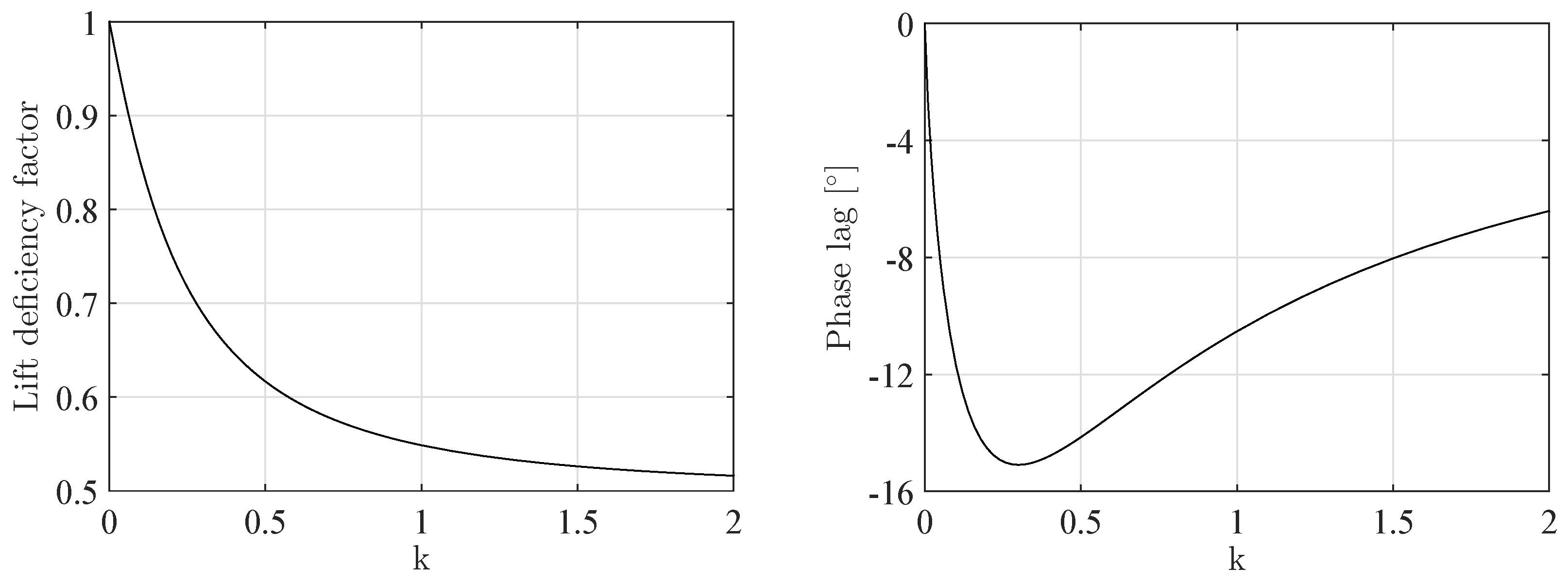
Figure 2.
Dry and wet fundamental blade frequencies of the Seiun–Maru propeller for different blade materials obtained with FEM and estimated with Equations (1) and (2).

Figure 3.
Structural frequency ratios for the various Seiun–Maru propellers.

Figure 4.
Geometry discretisation parameters for an unsteady propeller calculation. (Image republished from [19] with permission of the author.)
Figure 4.
Geometry discretisation parameters for an unsteady propeller calculation. (Image republished from [19] with permission of the author.)

Figure 5.
Comparison of dry (left) and wet (right) natural frequencies of the Boswell propeller blades from Young [7] and present work.
Figure 5.
Comparison of dry (left) and wet (right) natural frequencies of the Boswell propeller blades from Young [7] and present work.
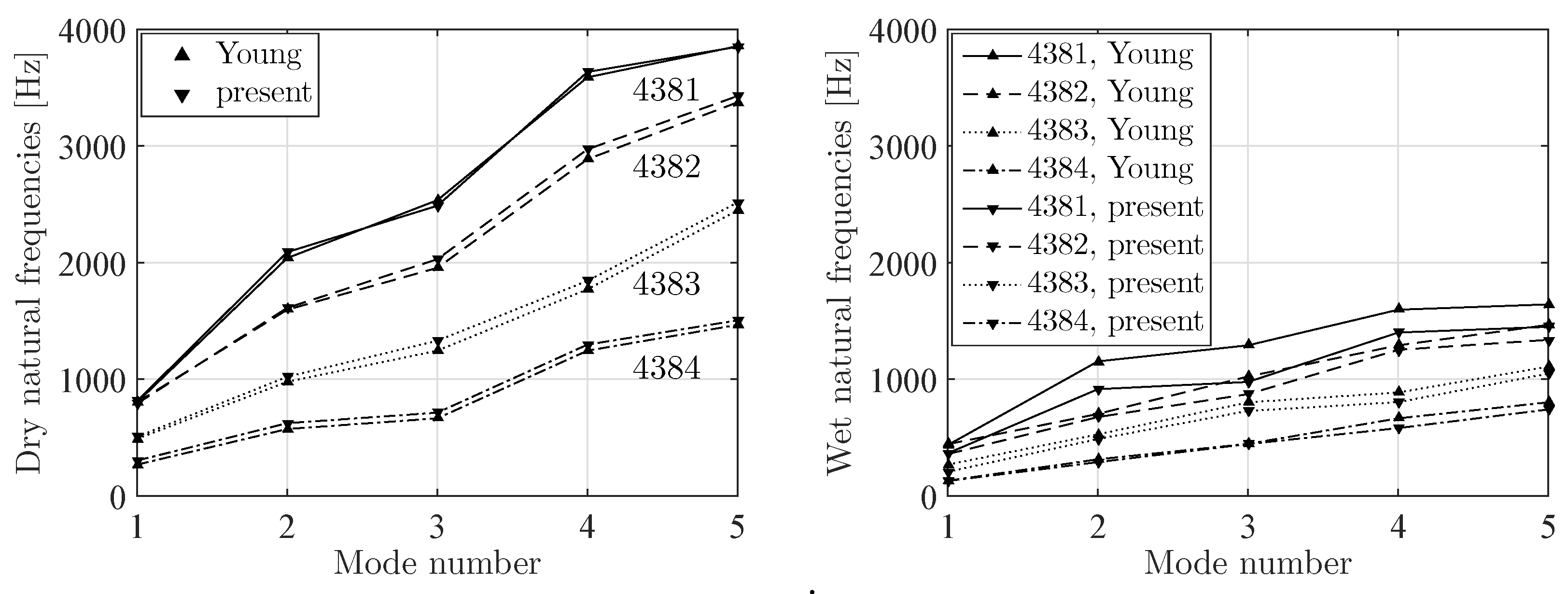
Figure 6.
Added mass and hydrodynamic damping of the hydrofoil for different plunge frequencies.

Figure 7.
Amplitude of non-circulatory and circulatory forces in plunge direction for different plunge frequencies.
Figure 7.
Amplitude of non-circulatory and circulatory forces in plunge direction for different plunge frequencies.

Figure 8.
Phase shift between non-circulatory plunge force relative to acceleration and circulatory plunge force relative to velocity for different plunge frequencies.
Figure 8.
Phase shift between non-circulatory plunge force relative to acceleration and circulatory plunge force relative to velocity for different plunge frequencies.

Figure 9.
Comparison of monolithic and coupling procedure solution of the predicted pitch motion, , as a function of the normalized time, , for rad/s (left) and rad/s (right) graph.
Figure 9.
Comparison of monolithic and coupling procedure solution of the predicted pitch motion, , as a function of the normalized time, , for rad/s (left) and rad/s (right) graph.

Figure 10.
Blade thrust (left) and tip displacement (right) results obtained with the FGD- and PGD-BEM model for various advance ratios. The subscripts and indicate with which BEM model the results were obtained.
Figure 10.
Blade thrust (left) and tip displacement (right) results obtained with the FGD- and PGD-BEM model for various advance ratios. The subscripts and indicate with which BEM model the results were obtained.

Figure 11.
Seiun–Maru ship effective wakefield. (Image republished from [19] with permission of the author.)
Figure 11.
Seiun–Maru ship effective wakefield. (Image republished from [19] with permission of the author.)

Figure 12.
Blade thrust computed with different BEM-FEM couplings for the glass–epoxy Seiun– Maru propeller.
Figure 12.
Blade thrust computed with different BEM-FEM couplings for the glass–epoxy Seiun– Maru propeller.
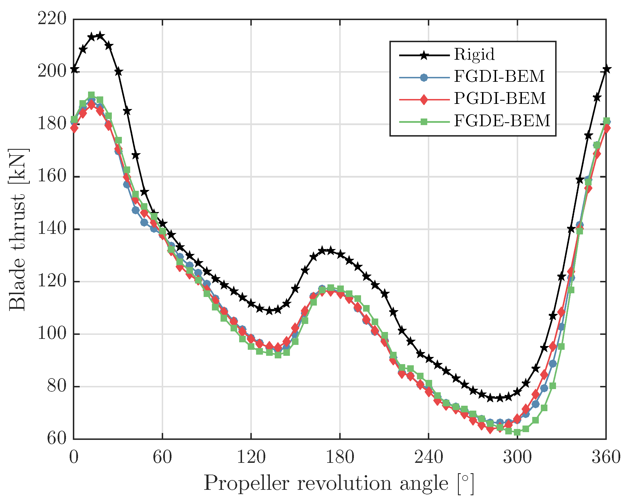
Figure 13.
Blade thrust computed with different BEM-FEM couplings for the carbon–epoxy Seiun– Maru propeller.
Figure 13.
Blade thrust computed with different BEM-FEM couplings for the carbon–epoxy Seiun– Maru propeller.

Figure 14.
Modal participation factors for the first three modes computed with different BEM-FEM couplings for the glass–epoxy Seiun–Maru propeller.
Figure 14.
Modal participation factors for the first three modes computed with different BEM-FEM couplings for the glass–epoxy Seiun–Maru propeller.

Figure 15.
Modal participation factors for the first three modes computed with different BEM-FEM couplings for the carbon–epoxy Seiun–Maru propeller.
Figure 15.
Modal participation factors for the first three modes computed with different BEM-FEM couplings for the carbon–epoxy Seiun–Maru propeller.

Figure 16.
Thrust reduction for minimum, maximum and average blade thrust calculated for the glass–epoxy (left graph) and the carbon–epoxy (right graph) propeller as obtained from the BEM-FEM coupled calculations.
Figure 16.
Thrust reduction for minimum, maximum and average blade thrust calculated for the glass–epoxy (left graph) and the carbon–epoxy (right graph) propeller as obtained from the BEM-FEM coupled calculations.

Figure 17.
Blade thrust, fluid added mass and hydrodynamic damping force computed with the FGDE-BEM-FEM coupling with and without including the fluid added mass and hydrodynamic damping in the calculations, for the glass–epoxy Seiun–Maru propeller.
Figure 17.
Blade thrust, fluid added mass and hydrodynamic damping force computed with the FGDE-BEM-FEM coupling with and without including the fluid added mass and hydrodynamic damping in the calculations, for the glass–epoxy Seiun–Maru propeller.

Figure 18.
Blade thrust, fluid added mass and hydrodynamic damping force computed with the FGDE-BEM-FEM coupling with and without including the fluid added mass and hydrodynamic damping in the calculations, for the carbon–epoxy Seiun–Maru propeller.
Figure 18.
Blade thrust, fluid added mass and hydrodynamic damping force computed with the FGDE-BEM-FEM coupling with and without including the fluid added mass and hydrodynamic damping in the calculations, for the carbon–epoxy Seiun–Maru propeller.

Figure 19.
Modal participation for first three modes computed with the FGDE-BEM-FEM coupling with and without including the fluid added mass and hydrodynamic damping in the calculations, for the glass–epoxy Seiun–Maru propeller.
Figure 19.
Modal participation for first three modes computed with the FGDE-BEM-FEM coupling with and without including the fluid added mass and hydrodynamic damping in the calculations, for the glass–epoxy Seiun–Maru propeller.

Figure 20.
Modal participation for first three modes computed with the FGDE-BEM-FEM coupling with and without including the fluid added mass and hydrodynamic damping in the calculations, for the carbon–epoxy Seiun–Maru propeller.
Figure 20.
Modal participation for first three modes computed with the FGDE-BEM-FEM coupling with and without including the fluid added mass and hydrodynamic damping in the calculations, for the carbon–epoxy Seiun–Maru propeller.

Figure 21.
Thrust reduction for minimum, maximum and average blade thrust calculated for glass– epoxy (left) and carbon–epoxy (right) propeller as obtained from the various FGDE-BEM calculations.
Figure 21.
Thrust reduction for minimum, maximum and average blade thrust calculated for glass– epoxy (left) and carbon–epoxy (right) propeller as obtained from the various FGDE-BEM calculations.


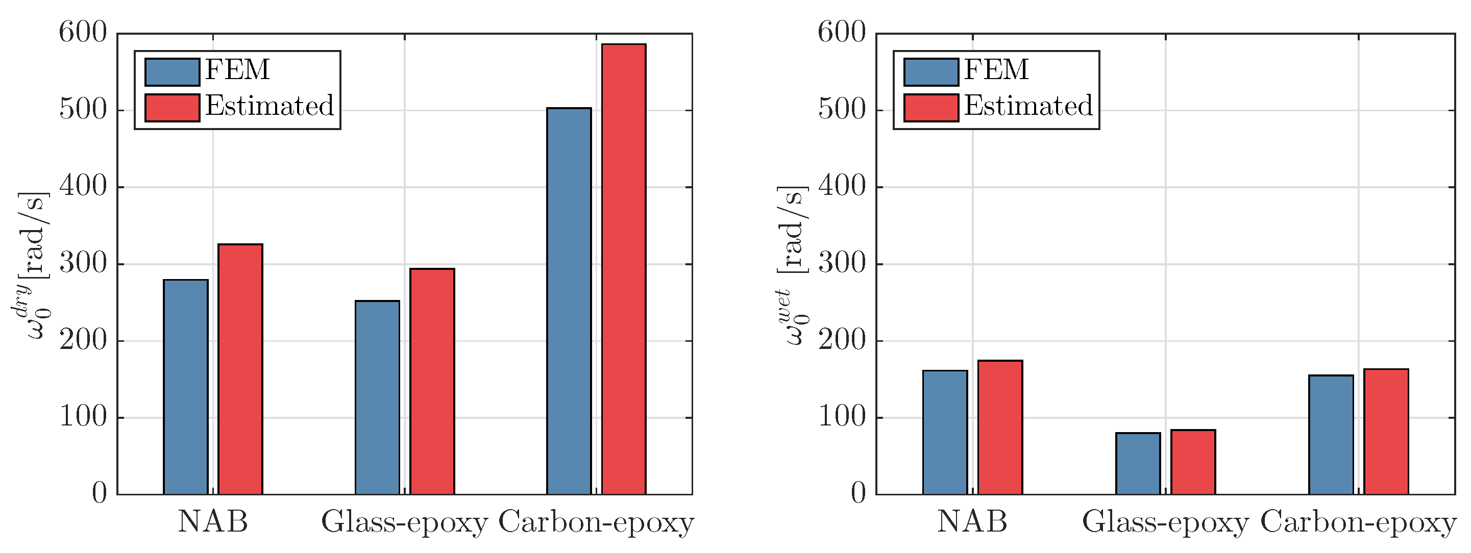
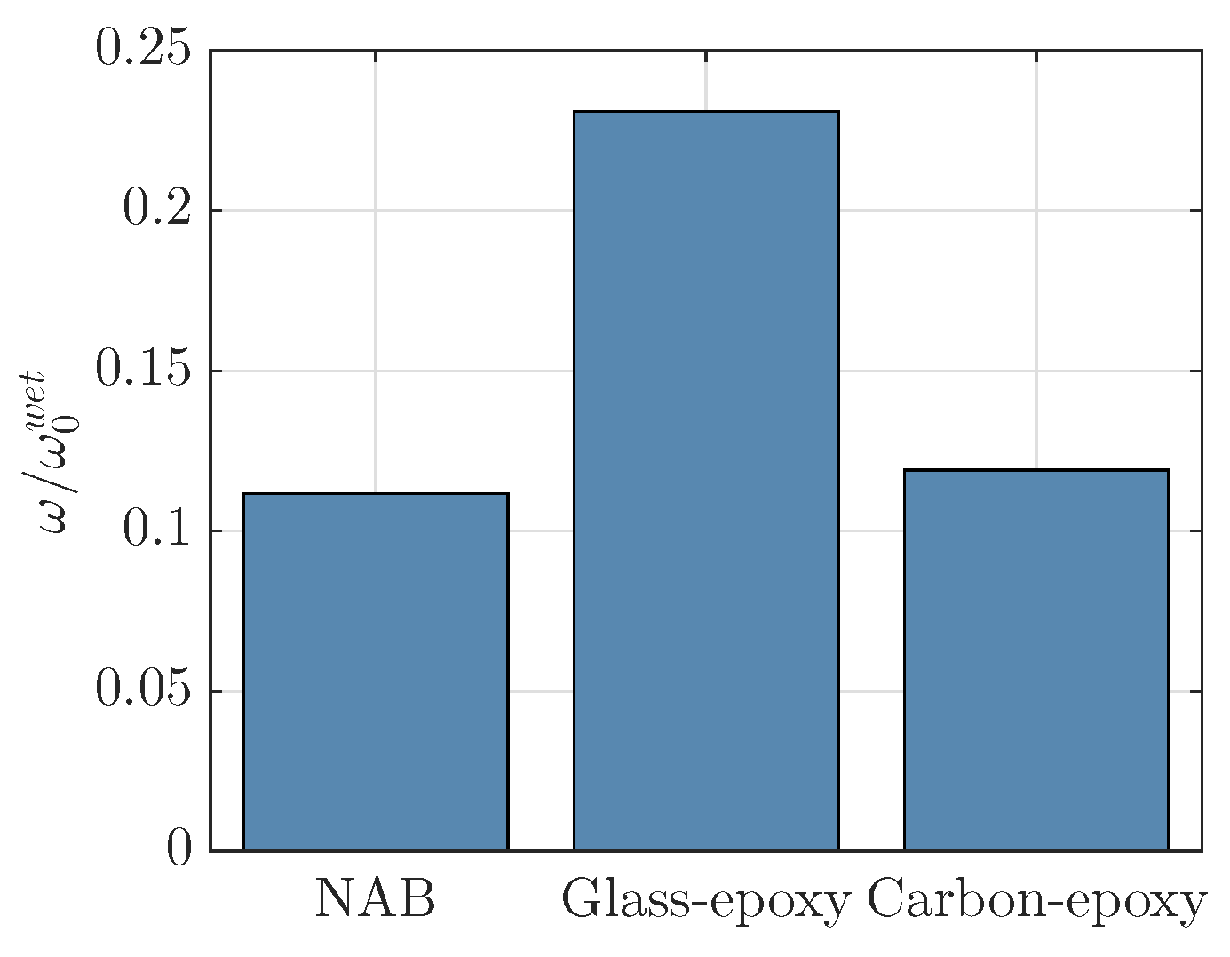
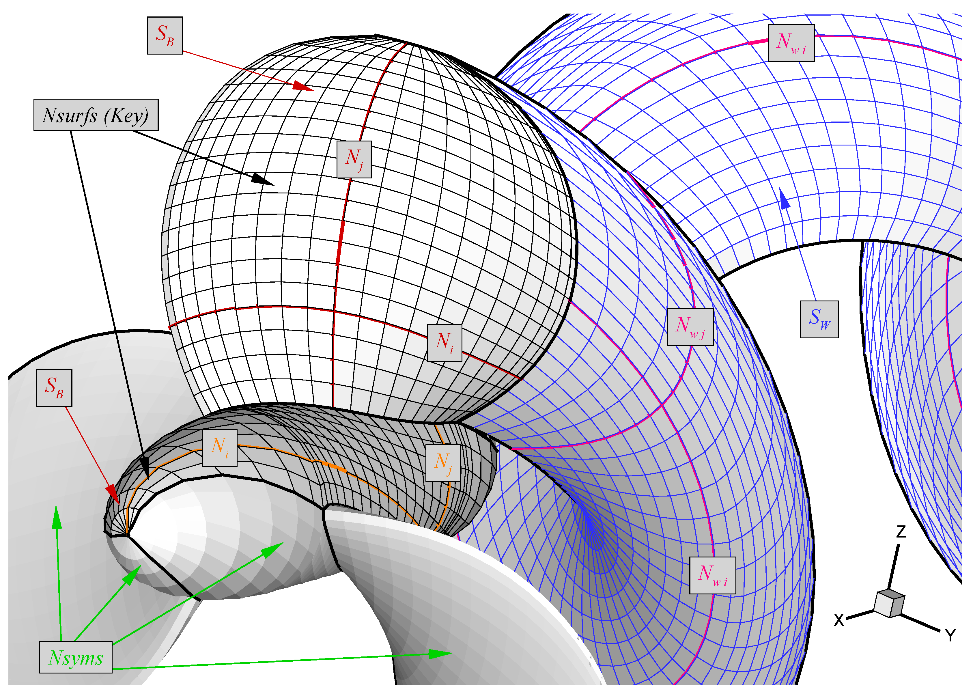
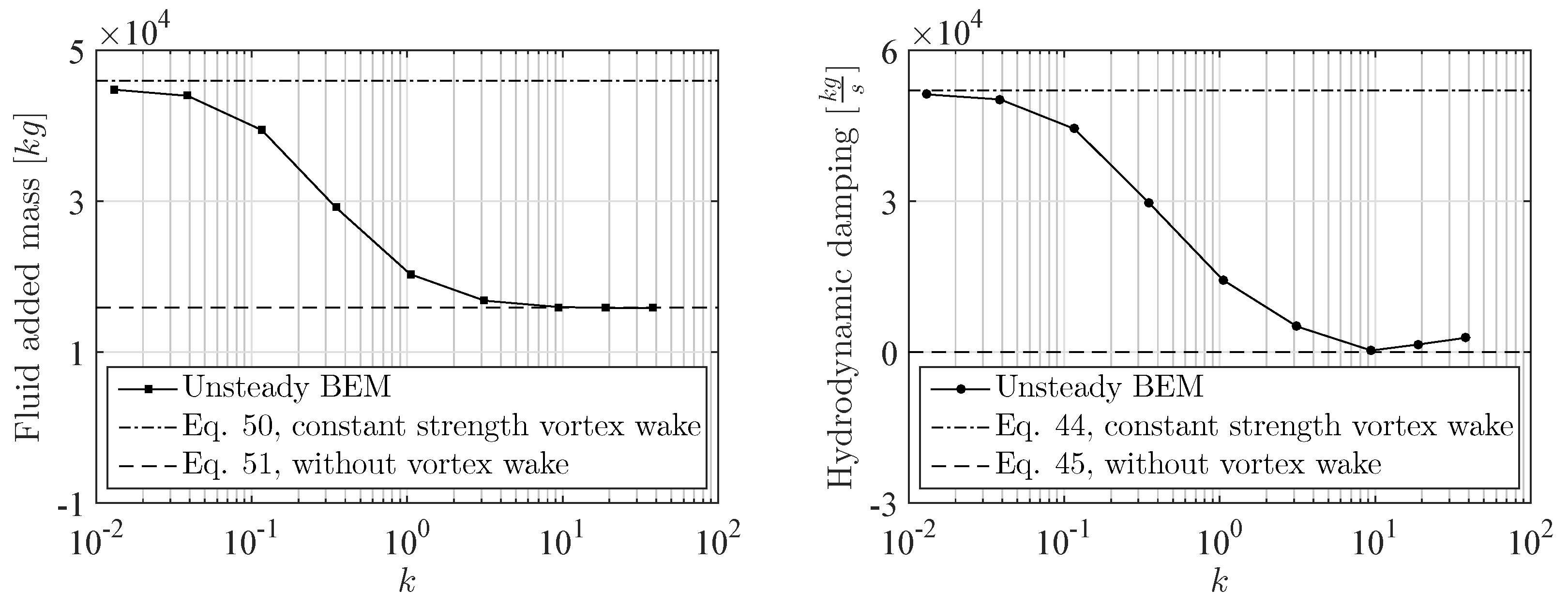
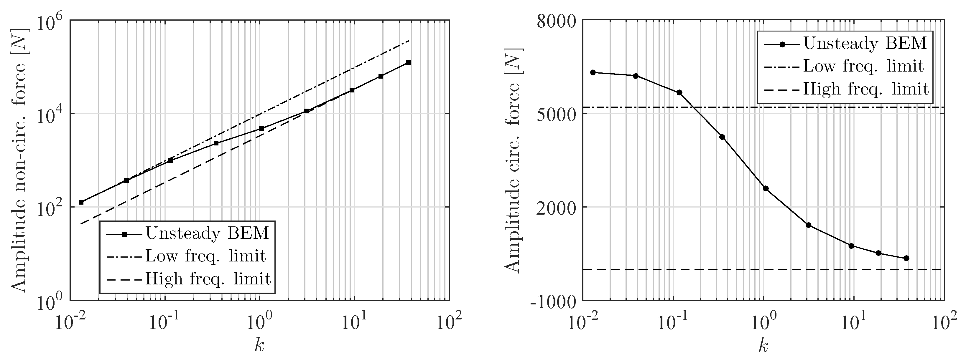
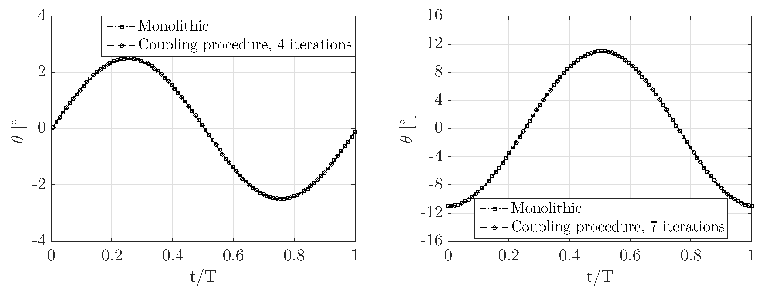
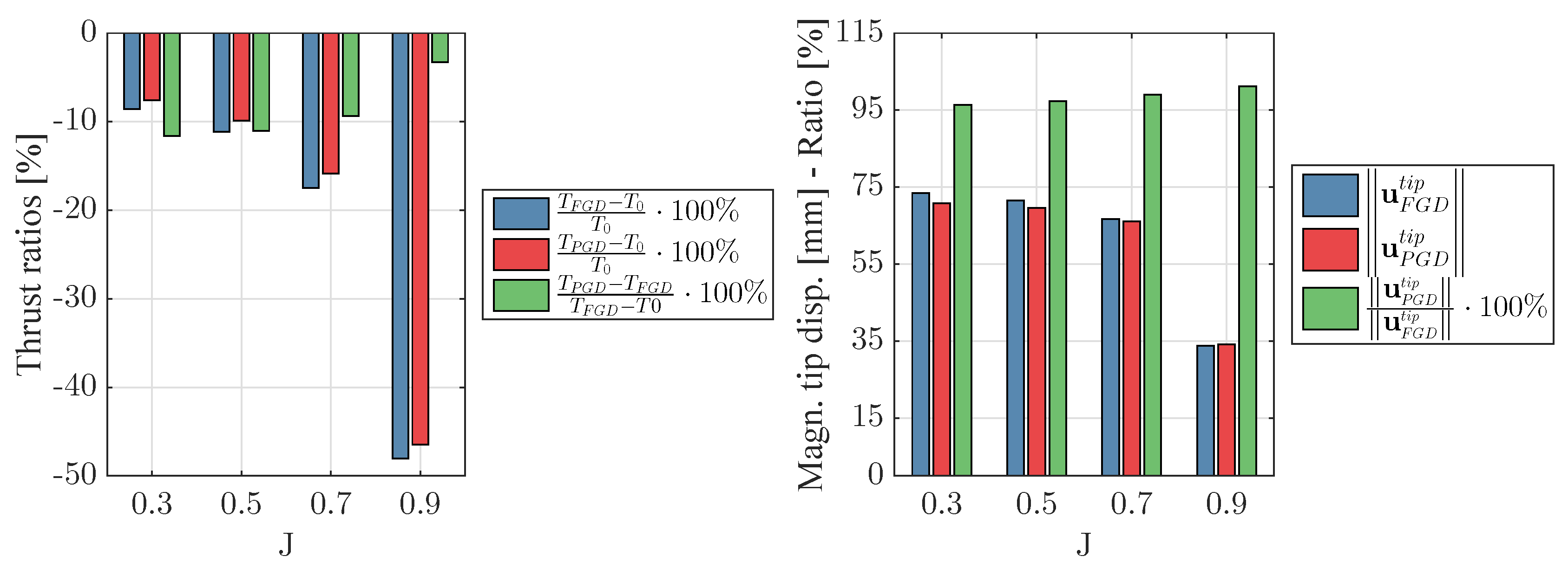
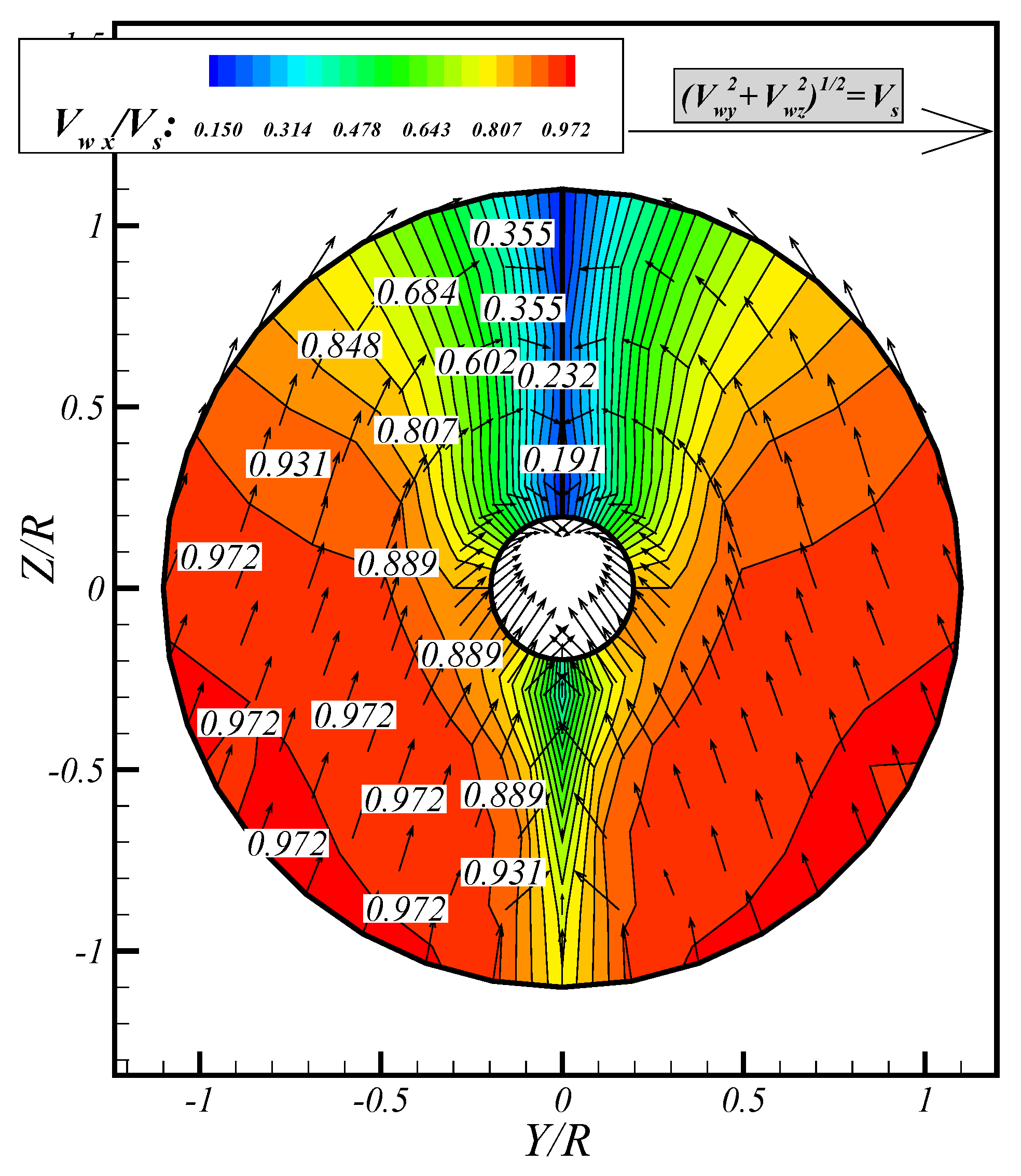
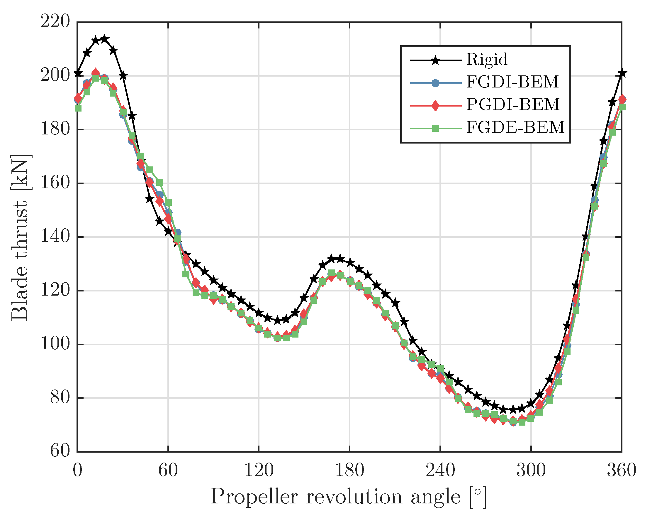
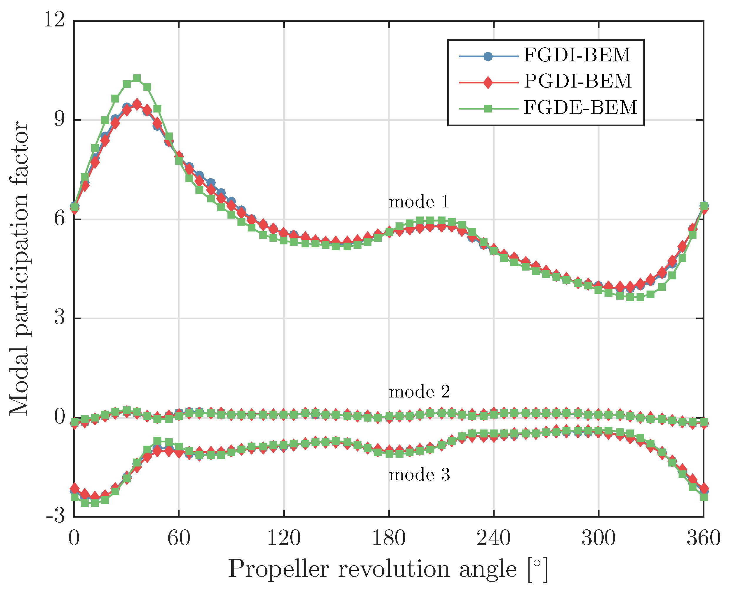
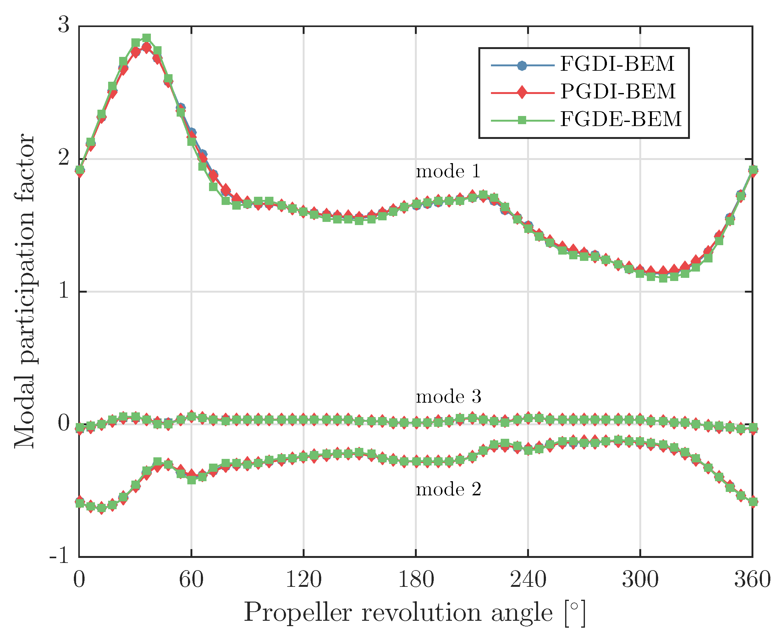
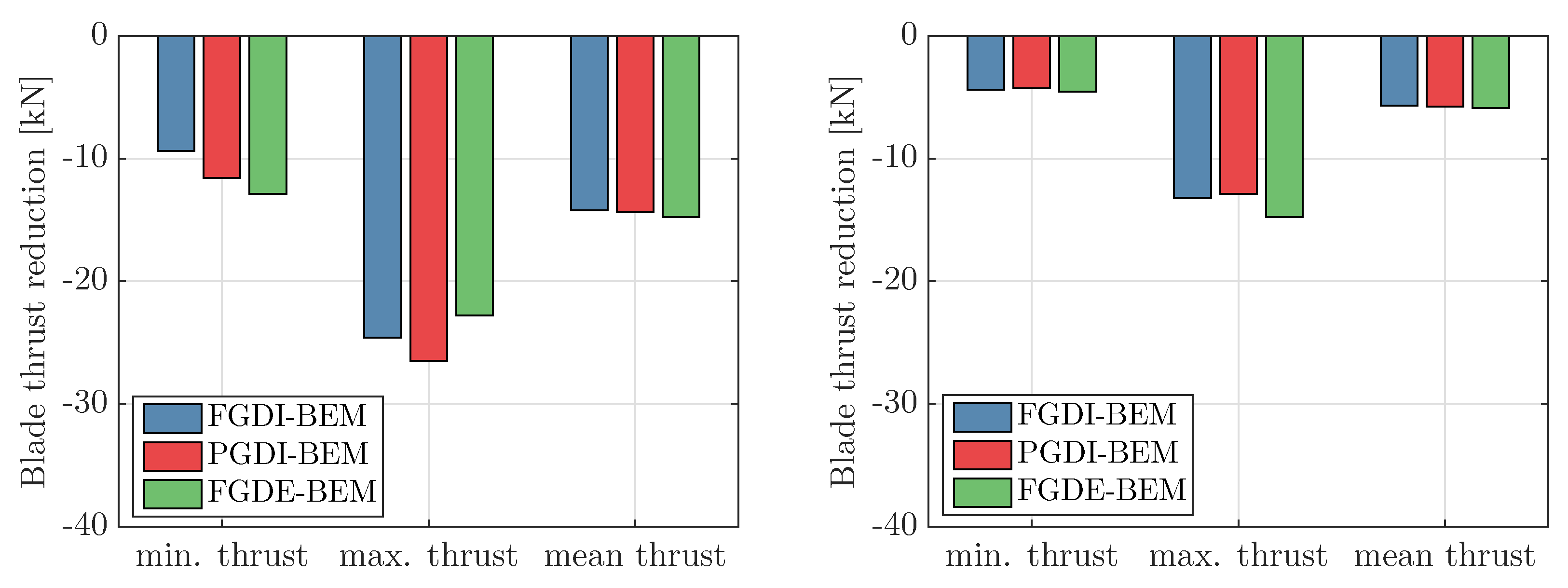
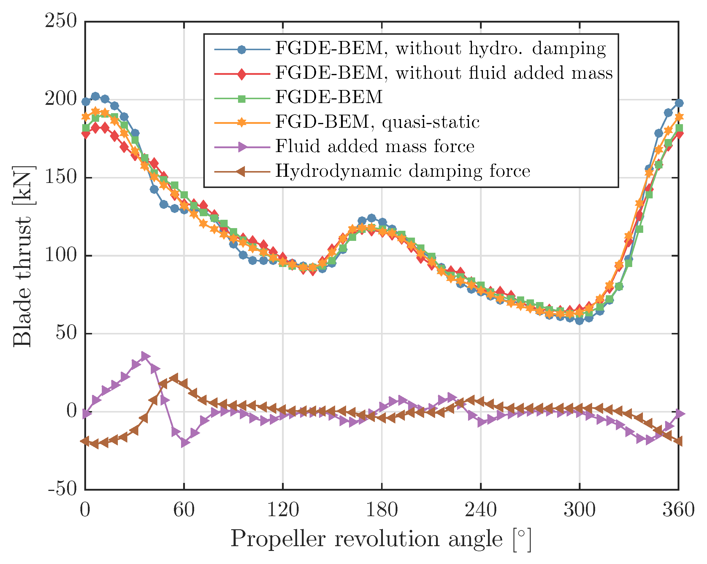
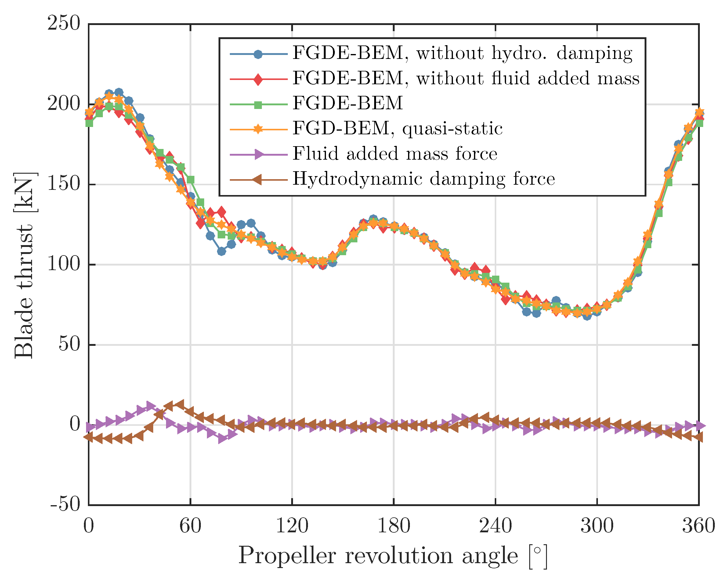
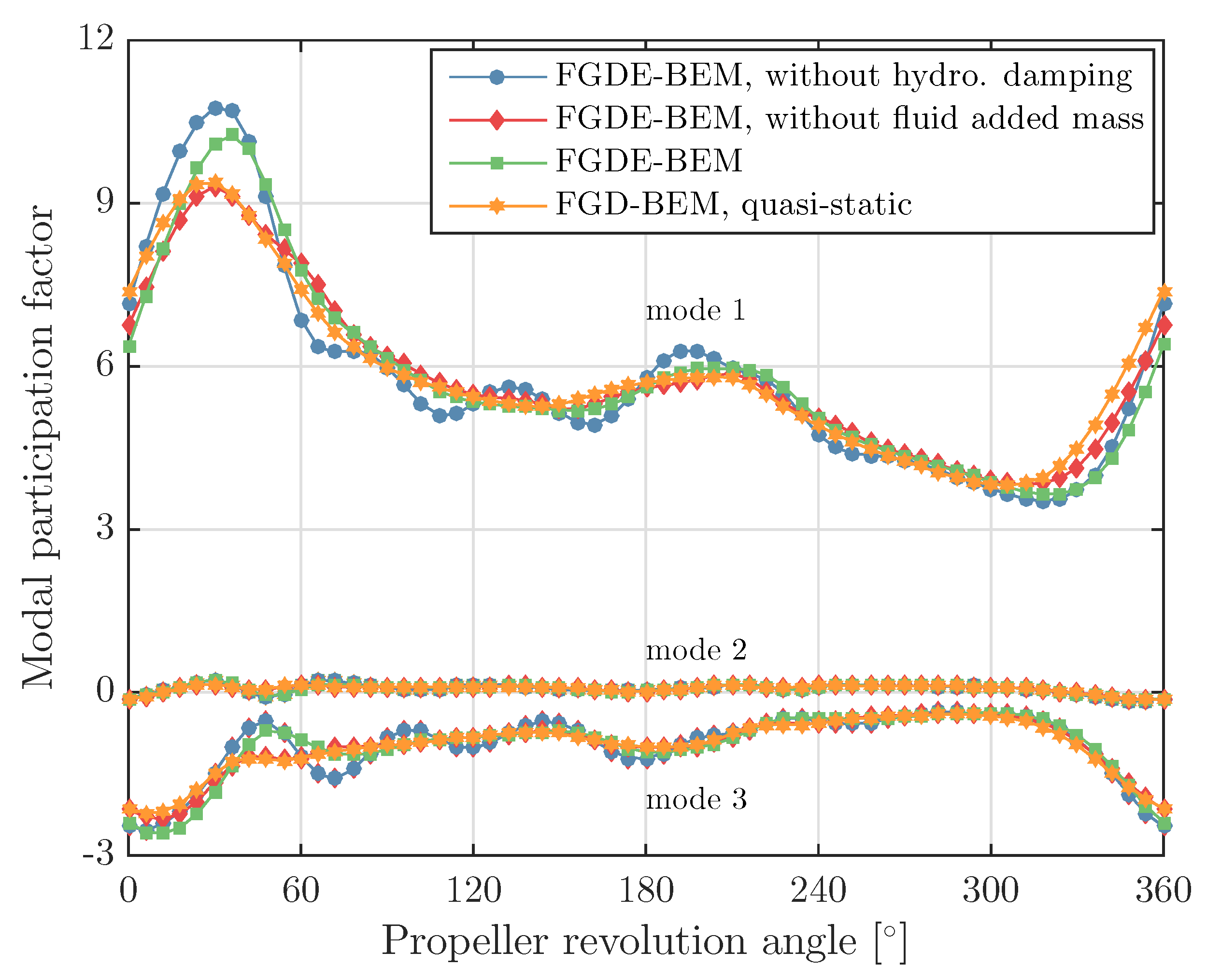
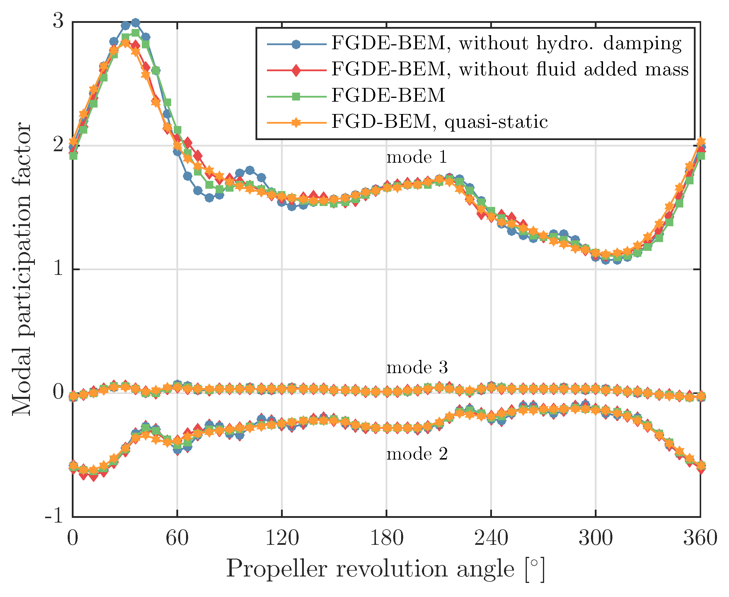
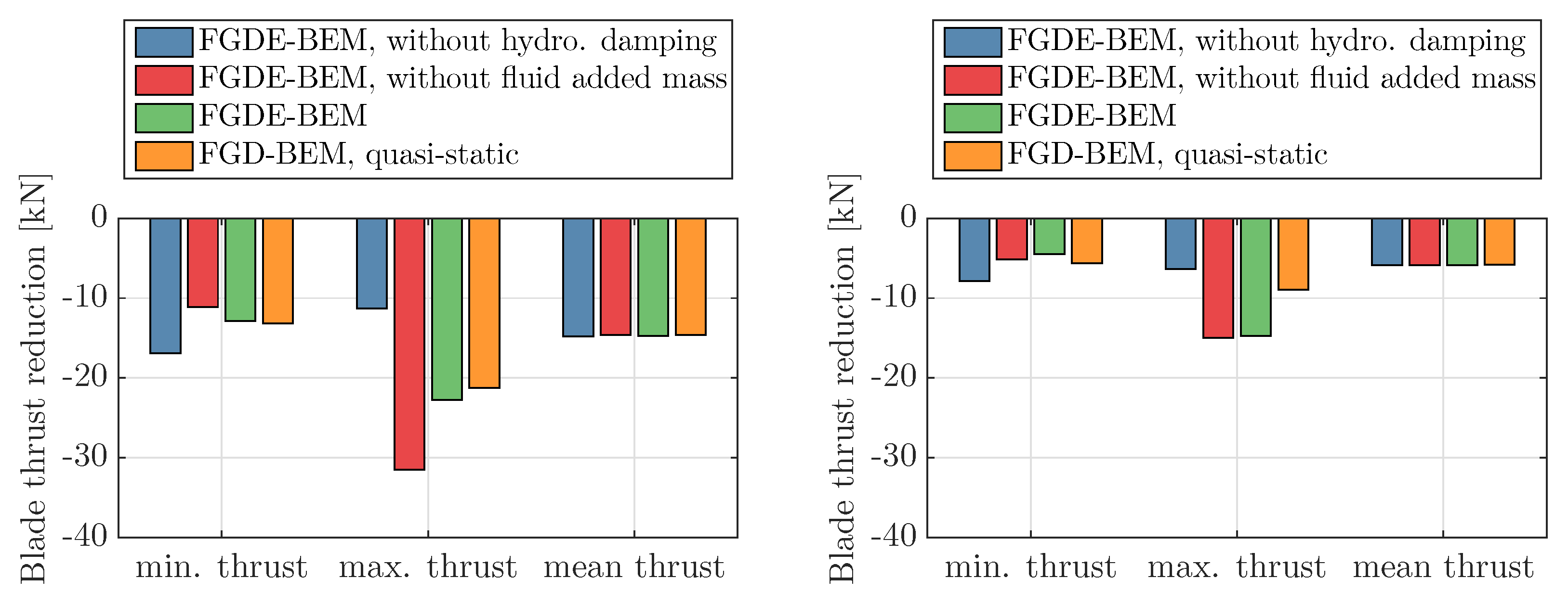
Table 1.
Main particulars of the highly skewed Seiun–Maru propeller.
| Diameter | 3600 mm |
| Pitch Ratio (mean) | 0.92 |
| Expanded Area Ratio | 0.7 |
| Number of Blades | 5 |
| Blade Thickness Ratio | 0.0496 |
| Boss Ratio | 0.1972 |
| Total Skew Angle | 45 |
| Rake Angle | −3.03 |
| Blade Section | Modified SRI-B |
Table 2.
Flow conditions for steady flexible propeller calculations.
| J | V (m/s) | (rpm) | (kN) |
|---|---|---|---|
| 0.3 | 2.98 | 165 | 96.6 |
| 0.5 | 5.72 | 191 | 96.0 |
| 0.7 | 9.97 | 237 | 96.2 |
| 0.9 | 19.6 | 364 | 97.3 |
© 2018 by the authors. Licensee MDPI, Basel, Switzerland. This article is an open access article distributed under the terms and conditions of the Creative Commons Attribution (CC BY) license (http://creativecommons.org/licenses/by/4.0/).
Share and Cite
MDPI and ACS Style
Maljaars, P.; Kaminski, M.; Den Besten, H. Boundary Element Modelling Aspects for the Hydro-Elastic Analysis of Flexible Marine Propellers. J. Mar. Sci. Eng. 2018, 6, 67. https://doi.org/10.3390/jmse6020067
AMA Style
Maljaars P, Kaminski M, Den Besten H. Boundary Element Modelling Aspects for the Hydro-Elastic Analysis of Flexible Marine Propellers. Journal of Marine Science and Engineering. 2018; 6(2):67. https://doi.org/10.3390/jmse6020067
Chicago/Turabian StyleMaljaars, Pieter, Mirek Kaminski, and Henk Den Besten. 2018. "Boundary Element Modelling Aspects for the Hydro-Elastic Analysis of Flexible Marine Propellers" Journal of Marine Science and Engineering 6, no. 2: 67. https://doi.org/10.3390/jmse6020067
Note that from the first issue of 2016, this journal uses article numbers instead of page numbers. See further details here.