Abstract
Major marine construction projects, resulting in the release of sediments, are subject to environmental assessment and other regulatory approval processes. An important tool used for this is the development of specialized numerical methods for these marine activities. An integrated set of numerical methods addresses four distinct topics: (1) The near-field release and mixing of suspended sediments into the water column (i.e., the initial dilution zone); (2) the transport of the suspended sediments under the influence of complex ocean currents in the far-field; (3) the settling of the transported suspended sediments onto the seabed; and (4) the potential for resuspension of the deposited sediments due to sporadic occurrences of unusually large near-bottom currents. A review of projects subjected to environmental assessment in the coastal waters of British Columbia, from the year 2006 to 2017, is presented to illustrate the numerical models being used and their ongoing development. Improvements include higher resolution model grids to better represent the near-field, the depiction of particle size dependent vertical settling rates and the computation of resuspension of initially deposited sediments, especially in relation to temporary subsea piles of sediments arising from trenching for marine pipelines. The ongoing challenges for this numerical modeling application area are also identified.
1. Introduction
In this paper, we present an overview of the development and applications of advanced numerical modeling of sediment transport and fate resulting from marine construction. This modeling is a useful tool to quantify the effects of these activities on the receiving environment. The modeling applications address a wide range of marine construction activities including: Dredging for the expansion of ports and harbors; disposal at sea of dredgates; trenching and backfilling for marine pipelines in shallow waters in approaching the coastline; and the removal and installation of underwater electrical cables.
In particular, we provide an overview of the modeling methods for their application in addressing environmental assessment and review issues. We present examples of the models for environmental assessment for port development and for construction of marine pipelines in the jurisdiction of British Columbia, Canada.
2. Physical Setting of British Columbia Coastal Waters
The British Columbia coastal waters extend over a distance of more than 900 km from the Canadian—United States border in the south, near the Port of Vancouver to the northern border between Alaska (U.S.) and British Columbia (Canada) in the north (Figure 1). The water depths range from up to 1800 m in the offshore continental margin to shallow waters in the inland seas such as Chatham Sound and the Strait of Georgia, with larger water depths in the deep inland fjords extending into the mainland. The physical forces acting on the ocean waters can be highly energetic [1] due to: Seasonally large winds (fall and winter); large tides, especially in the northern British Columbia (BC) waters; and major fresh water discharges, including the Fraser, Skeena and Nass Rivers (Figure 1).
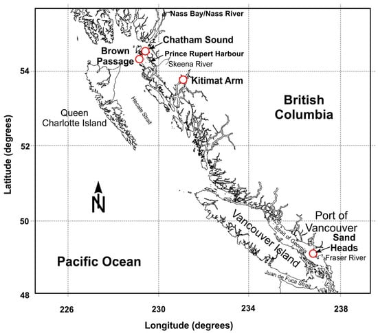
Figure 1.
A map of the British Columbia coast highlighting the areas where numerical modeling of sediment transport from marine construction has been carried out, from the Port of Vancouver in the south to Prince Rupert and Kitimat Harbors in the north as well as the Nass River Estuary in Northern British Columbia.
The large river discharges result in a high degree of density stratification of the water column which necessitates the use of 3-dimensional (3D) numerical models required to represent the vertical variations in ocean currents and other water properties such as temperature, salinity and density.
3. Environmental Assessment of British Columbia Marine Construction Projects
Marine construction projects have undergone more detailed levels of environmental reviews and assessments in recent decades to the point where environmental issues can present the greatest challenge in the project development process [2]. All marine construction results in environmental change and some of these changes may have negative consequences for some of the stakeholders who may be affected by the dredging project.
Environmental changes resulting from marine construction which are typically addressed include potential increases in suspended sediments in the water column, which can: Reduce visibility within the water column for fish and other animals that are seeking food prey; and decrease the penetration of sunlight available to marine vegetation. Increased suspended sediments can also detract from human usage of the marine areas for recreational purposes. Another environmental parameter of interest is an increase in the deposition of sediments to the seabed which may impact benthic communities and fish spawning usage of the seabed. In addition, sediment bound contaminants, if present in the marine construction area, may be released into the water column through the construction activities and may be subsequently be deposited at other locations. Guidelines for acceptable levels of increases in suspended sediment concentrations and sediment deposition are provided in the Canadian Council of Minister of the Environment (CCME) Canadian Water Quality Guidelines for the Protection of Aquatic Life [3]. Another aspect of environmental changes related to marine construction is the erosion of bottom sediments, which have been initially deposited due to marine construction, by unusually large near-bottom currents and their transport and fate in the marine environment. The changes in the sediment regime related to marine construction activities can be computed and quantified using numerical modeling methods presented below.
Major marine construction projects are subject to environmental reviews by governments through an environmental regulatory and permitting system. For projects in the province of British Columbia (BC) in Canada, the environmental regulatory system is shown as an organizational chart in Figure 2. The lead government environmental agency, usually the British Columbia Environmental Assessment Office (BCEAO), considers the inputs from many other government agencies, as well as from stakeholder groups including First Nations organizations and environmental non-governmental organizations, as well as private citizens, industry associations and others. For some projects, the federal government takes the lead role in the environmental assessment through the Canadian Environmental Assessment Agency (CEAA). In all cases, federal and provincial government agencies are involved in the expert review of evidence presented by the Proponent and its consultants in the application for the project.
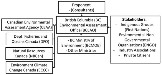
Figure 2.
An organizational chart for the Environmental Assessment Regime in British Columbia, Canada.
Following the first environmental review and assessment of the project, the construction phase of the project is required to follow the project plan and to address any conditions stipulated in the environmental review, including environmental monitoring during construction, and in some cases, following the completion of construction.
The environmental assessments of marine construction typically involve key government departments including Environment and Climate Change Canada (ECCC), the Canadian Department of Fisheries and Oceans (DFO) and the British Columbia Ministry of the Environment (BCMOE). For sediment transport and disposal issues in these assessments, ECCC and BCMOE have developed guidelines and in-house expertise that are specific to marine sediments including Disposal at Sea [4,5,6] and contaminated sediments [7].
4. Approaches to Numerical Modeling of Sediments Released from Marine Construction Activities
The advantage of using numerical modeling methods for sediment releases from marine construction projects is that the distribution of the released sediments can be quantified in considerable detail in terms of: (a) The time-varying distribution of the construction-released suspended sediments in the water column with location over the receiving area of the marine environment; (b) the spatial distribution of the construction-released sediments deposited onto the seabed; and (c) the potential for resuspension of these deposited sediments and their subsequent transport and fate for times of very strong ocean bottom currents. To ensure the validity of the highly detailed model outputs, the numerical models are subjected to calibration and verification analysis through comparison with field data.
An overview of the high level modeling approach for addressing the transport and fate of construction-released sediments, as used for environmental assessment purposes, is presented in Figure 3.
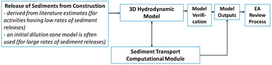
Figure 3.
An overview of modeling methods for addressing environmental assessment (EA) issues.
4.1. 3D Hydrodynamic Models
The 3D hydrodynamic model is at the core of the integrated numerical modeling approach to simulating sediment transport and fate. These advanced numerical models compute the 3D circulation and densities of the receiving waters into which the sediments from marine construction activities are released. The hydrodynamic model provides a computational fluid dynamics approach to the study of river, estuarine and coastal circulation regimes. These hydrodynamic models apply the full three-dimensional basic equations of shallow water hydrodynamics and conservative mass transport and solves for time-dependent, three-dimensional velocities, salinity, temperature, kinetic energy and mixing length and water surface elevation. The model is calibrated against field observations with adjustments made to some of the model parameters to improve the model performance. The most common adjustments are to horizontal and vertical diffusivity values, seabed bottom roughness and parameters determining the bottom friction.
Hydrodynamic models require extensive data inputs to force the computation of the ocean circulation and other dynamical properties within the 3D coordinates encompassing the model domain, i.e., within the model area and over the included water depths. The key data inputs are: Surface winds, provided as a surface boundary condition (SBC) in the model; tidal height data at the open boundary conditions (OBC) of model domain which allow the model to compute tidal heights and tidal currents within the model domain; and the volume of freshwater from major rivers entering the model domain on the appropriate open boundary condition of the model. The bottom boundary of the model is provided by bathymetric data which represents the depth of the seabed below the mean water surface level at each model grid. The variations in the water density, determined from ocean temperatures and salinities, within the model domain is also provided as data inputs to the model through specifying these values at OBC’s and as initial conditions within the model domain. Thus, surface heat flux (shortwave radiation, longwave radiation, latent, and sensible heat flux) and freshwater flux (evaporation, precipitation, and river runoff) may need to be considered in certain numerical studies. For some model applications, ocean waves within the model domain are also computed arising from the surface winds and by representing the incoming waves as open boundary conditions. Another dynamical factor affecting surface momentum and heat flux is sea-ice, although sea-ice is not present in most BC coastal modeling projects.
The horizontal grid system varies among the various available hydrodynamic models. Many of the models make use of a finite-difference rectangular grid system with some of these allowing for higher resolution representation of the circulation in sub-areas of the model domain through the use of nested horizontal grid systems. For the projects of the present study we have used two 3D hydrodynamics models.
The first approach, COastal CIRculation and SEDiment transport Model (COCIRM-SED) (Figure 4), is a highly-integrated, three-dimensional, free-surface, finite-difference numerical model code for use on rivers, lakes, estuaries, bays, coastal areas and seas [8,9,10,11] and consists of the circulation or hydrodynamic model as well as sub-modules which including multi-category sediment transport, morphodynamics, water quality and particle tracking, as discussed further below. It also includes wetting/drying and nested grid schemes, capable of incorporating tidal flats, jet-like outflows, outfall mixing zone and other relatively small interested areas. The gridding scheme in COCIRM uses:
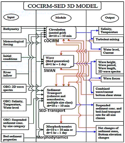
Figure 4.
Schematic diagram of the COastal CIRculation and SEDiment transport Model (COCIRM-SED) numerical model. OBC represents Open Boundary Conditions, SWAN is the Simulating WAves Nearshore ocean wave model [12] and dt is the user-selectable time scale range for which bottom elevations are adjusted in the Morphodynamics module.
- -
- in the vertical, either z layers (fixed size vertical layers which extend across the model domain) or sigma layers (a fixed number of vertical layers for each horizontal grid which is scaled according to the water depth in that grid), typically 10–30 layers.
- -
- and a rectangular horizontal grid size, typically ranging in size from 10–100 m.
The second approach is the well-known Delft3D model which supports a more flexible model gridding system than the finite difference grid. In particular, curvilinear orthogonal grids can be used to provide a high grid resolution in the area of interest and a low resolution elsewhere, thus saving computational effort. Delft3D [12] is an advanced suite of integrated numerical model components Figure 5), or modules, which can be combined with the Delft3D-Flow hydrodynamic model. Delft 3D is one of a handful of advanced deterministic (process-based) coastal ocean models, which are routinely used for this purpose [13].
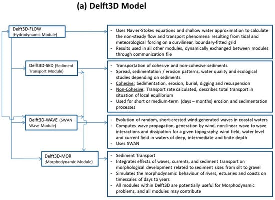
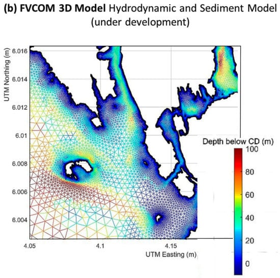
Figure 5.
(a) Schematic diagram describing the major modules of the Delft-3D model which uses the same inputs and outputs as the COCIRM-SED model system presented in Figure 4; and (b) an example of a Finite-Volume, primitive equation Community Ocean Model (FVCOM) for the Port of Prince Rupert which is presently under development.
More recently, the use of the unstructured Finite-Volume, primitive equation Community Ocean Model (FVCOM) model, which allows much higher horizontal resolution in the immediate vicinity of the construction activity, has been under development. FVCOM is a predictive, unstructured-grid, finite volume, free-surface Community Ocean Model, solving the 3-D equations of shallow water hydrodynamics and conservative mass transport [14], which provides modules to compute sediment transport and fate that are applicable to marine construction model applications. This very flexible gridding approach allows for very high resolution, i.e., small volume elements in the immediate vicinity of the construction activity where the sediments are being released, as well as providing much greater flexibility for representing very narrow ocean channels adjoining much larger water bodies connecting these channels to offshore areas. An example of the highly variable gridding system which can be used in FVCOM for the area around the Port of Prince Rupert is shown in Figure 5.
4.2. Release of Sediments from Construction
The release of sediments arising from marine construction activities is derived from technical documents on specific marine construction activities which are publicly available and from information provided by the marine construction operators and their equipment suppliers. Sediment releases are derived from the time varying rates of the mass and/or volumes of sediments arising from the construction activity which enter the marine receiving waters.
The nature of the sediments released into the receiving waters vary considerably according to the type of construction activity being much different for the mass and volumetric quantities of sediments released, and the rate of release. For example, for disposal at sea from large barges, this activity consists of very high volumes of materials being released, typically 2000 m3, with nearly 100% release of the sediments into the ocean through the bottom of the barge (Figure 6), over a short period of time of a few minutes. In contrast, the rate of release of sediment mass or volume into the receiving waters is much smaller, by three to four orders of magnitude, for mechanical dredging of the seabed as discussed below.
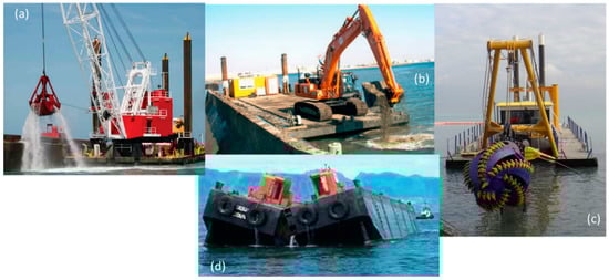
Figure 6.
Examples of marine construction equipment: (a) A clamshell bucket grab; (b) a barge-mounted backhoe; (c) a cutter suction head and support vessel; and (d) a split hull barge used for disposal at sea.
The particle size distribution of the sediments being discharged is an essential input to determine the rate and transport of the sediments within the water column. The particle size distribution is determined through laboratory analyses of surficial and sub-surficial sediment samples obtained in the vicinity of the marine construction activities where sediments are initially moved. Other key sediment properties are the density or specific gravity and the settling velocity of each sediment type. Density is determined from laboratory measurements and settling velocity, by each particle size, is determined from published tables which in some projects is augmented by laboratory measurements of collected sediment samples. All of these parameters are required by the Sediment Transport Computational Module (Figure 3) for each grid element of the Hydrodynamic Model which receives the released sediments at the model time steps in which the releases occur.
Dredging construction activities take many different forms which generally fall within two general categories of mechanical dredging and hydraulic dredging [15]. Mechanical dredgers use a grab or a bucket to loosen the in-situ material on the seabed and raise it to the surface (Figure 6). These come in different types with the most common types being bucket dredgers, grab dredgers and backhoe dredgers. Hydraulic dredging involves raising the loosened materials from the seabed in suspension through a pipe system connected to a centrifugal pump. Hydraulic dredging systems also have different types including: A suction dredger, a cutter suction dredger and a trailing suction dredger (Figure 6). Ongoing improvements in dredging systems are being realized to make the dredging operations more efficient [16] and more effective in reducing the loss of materials during handling and transport of the materials. The dredged materials can be loaded onto the ship from which the dredge is suspended and then later offloaded, or in the case of the cutter suction dredge, the materials can be discharged through a pipe to an ocean disposal area.
Trenching and backfilling of marine pipelines or underwater electrical cables represents a different marine construction activity in which sediments are released into the ocean receiving waters. Burial of the pipe or cable first requires trenching of the seabed which can be done by three different methods: Water-jetting, mechanical cutting or ploughing [17]. Once installed, the pipeline or cable can be backfilled in order to provide protection through either natural infilling or by artificial methods [18].
The key release parameters of mass and volume discharged, the rate of releases and the spatial distribution of the released sediments within the receiving water column has a very large range of possible values. As an example, for mechanical dredging, Hayes et al (2007) [19] suggest that the rate and mass of sediment resuspended during standard clamshell bucket dredging varied from 0.16 to 0.88% based on 5 field studies for estuarine and freshwater river environments. Burt et al (2007) [20] provide a higher range of estimated release rates for a specific dredging operation in a river with normal values being 3.35% but larger values of 5–6% were reported, and even very large transient values of 10% or more were noted. Given the large range in reported sediment release values from these mechanical dredging activities, the sediment release rate needs to be examined for each specific dredging operation according to the type of dredging operation being conducted in terms of the equipment in use, the physical and geotechnical properties of the bottom materials to be excavated and the operating conditions while dredging is underway.
4.3. Representing Sediments in the Numerical Models
The representation of the initial released sediments into the model must specify the fundamental properties of the sediments within the initial receiving volume of the model grid elements including particle size distribution, specific gravity and the settling velocities for each particle size. For subsequent model time steps, the model computes the changing suspended sediment concentrations within each grid volume element under the influence of horizontal transport by the local ocean currents and the vertical settling of the sediments, for each particle size category.
The models use high resolution grid sizes, relative to the requirements for the representation of ocean current, water level and water density features, of a few tens of meters, or smaller. This model horizontal resolution, combined with typical model time steps of a few to several seconds, allows the initial release of the discharged sediments to be initially diluted within a volume of one to a few model grid cells in the horizontal and over all or a subset of the model grid elements in the vertical within this horizontal subarea of the model. This simplifies, and in some cases, avoids altogether the need for initial mixing or dilution zone models (discussed below). For very small release rates, the representation of the released suspended sediment concentration (SSC) is correct as an average value over the full area and volume of the receiving grid element, although it does not identify the peak value of the sediment concentration within the grid element. As the suspended sediments further mix under the influence of ambient diffusion, negative buoyant spreading and advection by the ambient currents, the model representation of the peak SSC values tends to better represent the actual peak SSC values over mixing time scales of many minutes to a few hours.
The initial area and volume over, which the suspended sediments from construction activities occurs varies greatly, according to the type of construction activity being conducted. As an example, for mechanical dredging, having small release rates, the initial release typically extends over an initial release zone (IRZ), with has typical horizontal distances of one to a few tens of meters. The horizontal model resolution should match the distance scale of the IRZ. However, the size of this zone, especially for simulations of construction with small release rates such as mechanical dredging, is typically more uncertain than the rate of release of sediment mass or volume from the construction activity. Should the uncertainties in the IRZ distance scales result in the horizontal model grid size being larger than the IRZ size, the SSC values will be initially underestimated by the ratio of the horizontal grid size to the near-field zone distance scale. For the opposite case of the IRZ distance being somewhat being larger than one model grid size, the initial SSC values will be overestimated within the model grid receiving the sediment release. The effect of this uncertainty for the size of the IRZ to the horizontal model grid size is largest in the immediate vicinity of the construction activity; this is a very small area, that is highly disturbed from normal conditions due to the physical presence of the marine construction equipment and the associated acoustic noise in air and in the water.
For assessment of environmental effects from sediment releases, the changes in SSC and sediment deposition are more important in areas beyond the IRZ of the marine construction. Over the near-field zone consists of the plume area dominated by rapid settling velocities and large changes in SSC and sediment load. These changes are dominated by gravity settling with advection and diffusion also being important. The dimension of the near-field zone is typically occurring over a distance of about 100 m from the IRZ with associated time scales of up to one hour [21]. Within the near-field zone, the expansion of the area of the released sediments results in multiple additional horizontal model grid elements containing the released sediments, and a corresponding reduction in the SSC levels within the individual grid elements. As the vertical settling and advection-diffusive mixing proceeds through the near-field zone, the uncertainties in the model representation of the SSC values tends to decrease from the uncertainties in the IRZ. Beyond the near-field zone, the released sediments enter the far-field zone in which the plume varies more slowly, and advective-diffusive processes are as important as vertical settling.
In the examples presented below, the horizontal model grid size is selected to approximately match the estimated distance scale of the IRZ. The emphasis in the presented model outputs are on the changes in SSC and sediment deposition values beyond the immediate vicinity of the disturbed construction zone and the near-field zone. Often, the model output display results are presented and discussed for areas at distances from the construction zone of 100 to 300 m and beyond.
In contrast to mechanical dredging, the volume of the rates of sediment releases for disposal at sea from large barges, or high volume pipe discharges from cutter section dredging is typically much larger and can extend over many model grid elements. For these applications, an additional numerical model, in the form of an initial dilution zone (IDZ) model, is used to compute the initial SSC values and particle size distributions, which are then applied to the specification of sediments within the volume elements of the hydrodynamic model. For other types of sediment releases involving much high higher mass and volumes being released and much higher discharge rates, a 3D IDZ model is required. IDZ models are important especially with application to the disposal at sea of large volumes of marine dredgates from large barges or from pipe discharges with large volume fluxes, such as pipe discharges of dredgates from cutter suction dredging operations. Representing the release of large volumes of sediments can be addressed through specialized 3D models developed for this purpose. The IDZ models used in this paper are derived from two models which are part of the Automated Dredging and Disposal Alternatives Modeling System (ADDAMS) developed by the U.S. Army Corps of Engineers [22]. The Short Term FATE (STFATE), is a short-term fate model of sediment disposal, which is accepted by the U.S. Environmental Protection Agency [23]. The STFATE model can be used to simulate the short-term fate and near-field distribution of the disposal material released from large marine barges immediately following each disposal operation. The STFATE operates on the actual bathymetry using an identical or smaller model mesh to match the 3D hydrodynamic model grid, and typically is run over the initial tens of minutes of the disposal operation. STFATE simulates the dilution and dispersion of released sediments due to the gravitational descent, horizontal transport due to the ocean currents and turbulent diffusion and the rapid deposition of most coarse sediments with size larger than medium sand. The STFATE output provides the required information on the sediment releases to the 3D model hydrodynamic and sediment transport models, as well as the initial bottom accumulation in the immediate vicinity of the barge.
For discharges of released sediments through pipes, generated by hydraulic dredging methods, a different ADDAMS model, Continuous Discharge FATE (CDFATE) is used to simulate the initial dilution zone [24]. CDFATE is operated to simulate the distribution of suspended and deposited sediments for the pipe slurry discharge over a time frame of one hour or less under varying water depths and ocean current conditions. CDFATE delineates the horizontal spatial extent of the initial zone in which released sediments are present and the concentrations of the suspended sediments within this zone. To compute the vertical distribution of the sediment slurry from the pipe, and the amount of direct deposition during the initial 45 min of sediment disposal, the STFATE model was applied to the CDFATE results. The combination of CDFATE and STFATE simulations, where CDFATE provides the horizontal distribution and STFATE provides the vertical distribution (including direct deposition) provides a complete 3D representation of the SSC distribution for the initial dilution zone over the water column.
Other requirements for the computation of the transport and fate of sediments released from marine construction includes the representation of mitigation measures that can be conducted to limit the spatial extent of the SSC and deposition to the seabed in order to reduce environmental impacts. Two of these mitigative measures are the use of silt curtains and sheet piles located in the immediate vicinity of the marine construction activity. Realistic simulation of the effects of these mitigation measures requires the use of horizontal grids having horizontal grid dimensions of 20 m or less. Even for such fine grid sizes, the location of silt curtains may be displaced by a distance of a few to several meters from their actual location relative to the construction activity.
4.4. Sediment Transport Computational Module
The sediment transport computation module simulates the sediment dynamics of the released suspended sediments, separately for a set of discrete sediment particle size categories, typically numbering from 3–8. In the COCIRM-SED modeling framework, for fine-grained sediments with particle sizes less than 32–62 μm (clay–silt range), modeling of cohesive sediment transport is applied, while for coarse sediments with particle sizes of 32–62 μm (coarse silt, sand, granule and fine pebble), modeling of non-cohesive sediment transport is used. The vertical settling velocities for each sediment particle size category are derived according to laboratory and textbook results. Two separated parts are involved in coarse sediment transport, namely suspended-load and bed-load. The deposition of suspended sediments onto the seabed and the erosion of the deposited sediments off the seabed are also represented according to turbulent sediment dynamical methods derived from laboratory and widely accepted sediment-related hydraulic engineering methods. The morphological or morphodynamic module solves for the bottom elevation variations due to sediment deposition and erosion over the duration of the modeling.
The details of these computations for the modeling systems used in the present study are described in detail in References [10,12]. Evaluation of the environmental effects derived from the outputs from the modeling of the sediments released from marine construction activities are facilitated by comparisons with the SSC, and sediment deposition rates under natural conditions for the study area. The sediment regime of the natural environment can be represented through SSC and sediment deposition rates realized from observations or from sediment background models which use similar methods to those of the present study (e.g., Reference [25]).
5. Examples of Numerical Modeling of Sediments Released from Marine Construction Activities
A partial list of numerical modeling studies conducted in support of the environmental assessment for major marine construction projects proposed for the coastal waters of British Columbia from the year 2006 to 2017, is presented in Table 1. These eight studies illustrate the diversity of the marine construction activities, in terms of the type of construction activity simulated, the attributes of the 3D model used and the Initial Dilution Zone (IDZ) models that were applied. In all of these studies, numerical modeling of sediment releases played a key role in quantifying the effects on the marine environment.

Table 1.
A list of selected sediment modeling projects for the transport and fate of sediments released from marine construction projects off the coast of British Columbia conducted over the years 2006 to 2017.
In the remainder of this section, for three of these studies, we present descriptions of the modeling approach used and examples of the model outputs which were used to inform the environmental assessment of the projects.
5.1. Marine Dredging in Porpoise Channel of Chatham Sound
The first example is from the BC North Coast in the vicinity of the Port of Prince Rupert within the extended area managed by the Prince Rupert Port Authority. This dredging operation was simulated to occur over a period of 153 days from January to June. The model domain includes southern and central Chatham Sound, a shallow inland sea, with the construction type being dredging the sea bed in Porpoise Channel off Lelu Island, in order to build a marine offloading facility for a proposed Liquified Natural Gas (LNG) project on Lelu Island. This involves dredging of 615,000 m3 of bottom materials for construction of a materials offloading facility in Porpoise Channel, the resolution of the COCIRM-SED model [28] is 30 m in the vicinity of the dredging area including Porpoise Channel and adjoining areas, within a 210 m horizontal grid over the remainder of the model domain Figure 7. The vertical resolution was 12 z-layers. Z-layers rather than sigma layers were used for this model application because of the high degree of vertical stratification within the water column in the model domain due to the direct discharges of the Skeena River. This high level of vertical stratification could result in instabilities to the model computations, especially near open boundaries, if using sigma layers in such a highly stratified hydrodynamic regime.
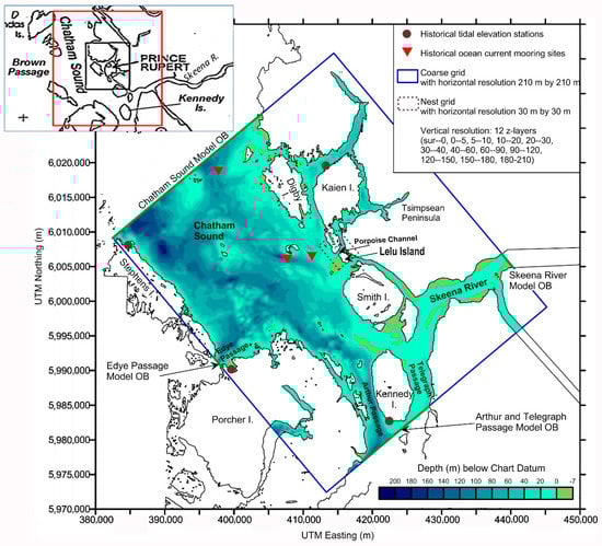
Figure 7.
The model domain, open boundaries (OB), water depths and locations of current meter data sets used in model verification for the numerical sediment transport model for dredging in Porpoise Channel.
The COCIRM-SED model was forced at the open boundary conditions by tidal levels. The Skeena River discharge was specified as an input to the southeast open boundary of the model. Wind forcing is applied through the surface boundary condition and the stratified water properties within the model are determined from historical DFO conductivity temperature depth (CTD) water properties data sets. Both COCIRM-SED models were calibrated and validated using comparisons to DFO current meter data sets (locations shown in Figure 7) with overall good agreement between the model and observed currents [28].
In this simulation, the loss rate was taken to be 1% so as to be on the conservative side based on studies by [18] for releases from a bucket dredge. These releases were represented as one-half of the total loss occurring within 5 m of the bottom due to a combination of: Capturing the sediment, expulsion of sediments when closing the bucket, and during the initial raising of the bucket through the water column. The remaining 50% of the losses are assumed to be evenly distributed through the upper water column. The mass discharge rate of the released sediments, as computed individually for each of six particle size categories, were input directly into the z-layers of the 30 m horizontal grids that were occupied by the dredging unit.
The model outputs provided for the environmental assessment process included the predicted distribution of Suspended Sediment Concentration (SSC) during the course of the dredging operations (see an example of the model derived SSC values for a large flood and large ebb tidal flow in Figure 8) and the deposition of the sediments released by dredging onto the seabed, as shown in Figure 9. The highest SSC’s of 16–17 mg/L are in the immediate vicinity of the dredging, within 200 m, while the adjoining areas within about 1 km have SSC levels of 1–5 mg/L. Otherwise, the SSC values are below 1 mg/L which is well below natural background levels.
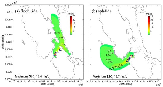
Figure 8.
Model-derived suspended sediment concentration (SSC) (mg/L above background, maximum value in the water column) for (a) a flood tide and (b) and ebb tide. Numbers mark depths (above seabed) of maximum values in vertical column. Blue contours present the areas of SSC greater than 5 mg/L.
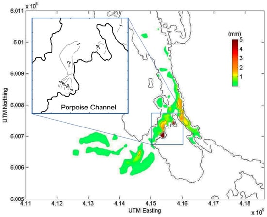
Figure 9.
Model derived deposition onto the seabed in Porpoise Channel and the surrounding area after 30 days of dredging activity in January. The line contours are for values of 1, 2 and 5 mm.
The sediment models are also used to compute the net deposition resulting from the 30 days of dredging (Figure 9). Here we see that the maximum deposition is 0.11 m, which is confined to within 50 m of the immediate vicinity of the disturbed dredging area. Outside of the immediate area of dredging the sediment depositions amount to 0.01–0.025 m in the confined areas of Porpoise Channel, extending inland to the mainland coast. Otherwise, deposition levels are very low at less than 0.002 m (or 2 mm) which are well below background levels which are related to deposition from the Skeena River sediments and natural transport of sediments.
5.2. Disposal at Sea of Dredged Sediments in Brown Passage
This example of numerical modeling of sediment transport is from Brown Passage, which connects the inland sea of Chatham Sound to the deeper Pacific Waters of Hecate Strait and Dixon Entrance [29]. The construction activity simulated is for ocean dumping from barges for disposal of dredged sediments at a proposed site in approximately 200 m water depth (Figure 10). The disposal from the barge has a volume of 2400 m3 which occurs over a 2 min duration, with barge disposals being repeated every 8 h and 43 min.
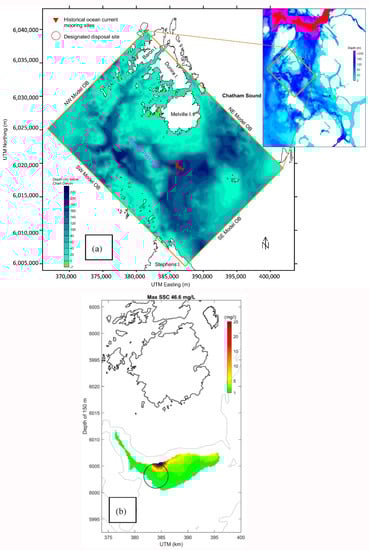
Figure 10.
(a) The Brown Passage model domain and its water depths and (b) a sample of the model results for the sediment plume at 150 m depth realized from the disposal at sea operations. Areas with SSC greater than 25 mg/L are marked by blue color. The black circle marks a previously used ocean disposal site (1 nautical mile in diameter).
The COCIRM-SED finite difference model was used over the domain shown in the map and with a horizontal resolution of 100 m and a vertical resolution of 22 sigma layers [25]. The use of sigma layers was suitable for this model application because the density stratification of the water column within the model domain was smaller than for model domains which include direct inputs from major river discharges. The model was forced at tidal height elevations spanning four open boundaries and by hourly surface winds. The four model open boundaries include the four adjoining sides of Brown Passage (Figure 10). Tidal elevations at these four open boundaries were derived from 7 major tidal height constituents (O1, P1, K1, N2, M2, S2, K2) using the DFO standard tidal prediction program. Wind forcing is applied through the model surface boundary conditions using wind data measurements at the nearby Lucy Island weather station. The initial temperature and salinity distribution within the model domain are derived from DFO historical CTD measurements [29].
The STFATE IDZ model was used to represent the short term distribution of the sediment releases as input to the 3D hydrodynamic model. The STFATE model results show that during the initial 45 min of each disposal trip, the sand settles more quickly than clay or silt. The suspended sediment is mostly concentrated within 10 m of the bottom. Moderately high levels of clay and silt (50 mg/L) are predicted at depths around 150 m above the seabed (i.e., at 50 m water depth), and moderately high levels of sand (70 mg/L) are predicted from approximately 20–80 m above the seabed (i.e., at 120 to 180 m depth).
One snapshot of the sediment transport model results for SSC is shown at 150 m depth (Figure 10). Here we see maximum SSC value of 46.6 mg/L in the immediate vicinity, within 500 m, of the barge disposal location. The SSC values extend in the form of a subsurface plume eastward from the previously used disposal site to a distance of a few kilometers with SSC values that are generally less than 5 mg/L.
5.3. Trenching for a Marine Pipeline in Nass Bay
This example of sediment transport modeling is for trenching conducted for a marine pipeline project in the shallow waters of Nass Bay of the Nass River Estuary in northern BC [33]. Here we see (Figure 11) the water depths in the model domain (left) and the horizontal grids in the Delft3D-SED model with 35 m resolution except for a higher resolution of 10 m in the pipeline corridor along southern side of Nass Bay. In the vertical, 10 sigma layers were used. For this model application, sigma layers were found to be suitable even with the direct input of freshwater from the Nass River into Nass Bay, because the water depths in Nass Bay are comparatively shallow which allows sigma the absolute depths of the sigma layers to vary less than would be the case where there is a large range in the total water depth within the receiving waters of the low density river water inputs. The forcing for the Delft3D hydrodynamic model is tidal heights and salinities obtained from time series measurements at the single open boundary at the Nass Bay entrance to Portland Inlet. The discharge from the Nass River obtained daily river data from Station ‘Nass River above Shumal Creek (08DB001)’, recorded by the Environment Canada and available online, is used for the eastern open boundary of the model. Salinity conditions required to initialize the model were obtained using transect data from boat-based CTD profile data across the mouth of Nass Bay as well as at interior locations in Nass Bay and Iceberg Bay. Winds forcing was provided by the Environment Canada Meteorological Service (ECMSC) using the High Resolution Deterministic Prediction System (HRDPS). The Delft3D hydrodynamic model was validated using ocean current observations obtained from an Acoustic Doppler Current Profiler (ADCP) instrument mounted on a subsurface mooring located at 22.5 m water in southwestern Nass Bay during a model verification run for a 25-day period in November 2015 [33].
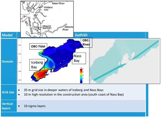
Figure 11.
The model domain, including water depths and the horizontal grids, for the Delft3D sediment transport model used to simulate the fate and transport of sediments from trenching and backfilling for marine pipeline construction in Nass Bay.
The sediments released from the trenching operation were derived for the case of two mechanical bucket dredges operated simultaneously from the center of the marine pipeline corridor moving in opposite directions. The total width of the trench is taken as 33 m with 1:5 sloping sides spanning 15 m on either side plus a flat segment of 3 m width. Handling losses as the sediment is trenched and then dumped either onto a spoil pile directly or in intermediate locations are taken as 3% for each time the material is moved. The 3% release rate is at the large end of the possible range of release rates so as to avoid any possibility of underestimation of sediment releases in the absence of a definitive design for this construction activity. This release rate is applied over the full water column since water depths relative to the low tide water levels are small being about 1 m or over nearly all of the pipeline route.
A representative example of the sediment model results is provided a snapshot of the SSC values at the end of flood tide (Figure 12). Here, the highest SSC values occur within 50 m of the two dredging barges reaching values of up to 66 mg/L. These large SSC values were limited to areas within 50 m of the dredging barges with much lower values of 1–5 mg/L extending to distances of 100–200 m, beyond which the SSC values were very small at <1 mg/L. In the areas beyond 50 m from the dredging barges, the SSC values are generally considerably less than the natural background SSC values in Nass Bay associated with the high turbidity of the Nass River waters within Nass Bay and the natural episodes of bottom sediment resuspension associated with very large tidal currents in the shallow waters of Nass Bay [33].
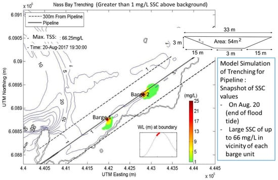
Figure 12.
Model derived simulations of suspended sediment concentrations for trenching of the Nass Bay pipeline by two clamshell dredge units.
6. Summary and Discussion
The use of integrated 3D sediment transport models provides a useful method to simulate the suspended sediment concentrations and deposition onto the seabed of sediments released from marine construction activities. The 3D models have horizontal grid resolutions of typically 10–30 m (for dredging and for marine pipeline construction) and 100 m (for ocean disposal at sea) with vertical resolution of 10–30 layers over the water column.
The sediment transport modeling provides quantitative and highly detailed depictions of the SSC distributions in all three dimensions under time varying forcing by tides, winds and river discharges. It also provides detailed two dimensional maps of the deposition of the released sediments resulting from the marine construction activity. These model outputs inform the environmental assessments of the marine construction project by allowing the effects of the marine construction to be estimated on the natural marine ecosystem, including marine vegetation, benthic communities and fishing activities.
The results of the sediment transport models can be used to develop more environmentally effective and efficient marine construction plans and to test the effect of mitigative measures such as sheet piles and silt curtains. The effects of mitigative measures is carried out by operating the model with and without the mitigative measures. The effect of silt curtains was tested through model runs for the two projects conducted in Kitimat Harbor (Table 1) and the model results provided information on the reductions of, and areal extent for, the SSC and deposition values resulting from the use of silt curtains. 3-D modeling is useful in quantifying the effects of mitigative measures and in optimizing the results achieved from these measures. In a similar fashion, variations in the way the construction activity is conducted can be simulated through model runs by computing the effect of changes in the construction plan on the resulting SSC and sediment deposition.
Further progress for this type of sediment transport and fate modeling can be achieved through the use of even higher resolution models through variable grid sizes which would allow very high resolution in the immediate vicinity of the marine construction activity where the sediments are released. The improvement in horizontal resolution reduces the reliance on the use of initial dilution zone models which have their own uncertainties and increase the effort for the overall modeling process. The use of unstructured finite volume models represent an approach to achieving the very high resolution being sought.
Another area of improvement would be to have more accurate inputs to the models on the sediment releases from construction activities, including more data on wider range of construction activities and the evolving equipment and operations within each type of construction activity. The improved sediment release information could be achieved by in-situ and laboratory-derived measurements of sediment releases during the operation of the equipment in the marine environment. The in-situ studies would include measurements of the mass and volumetric rates of sediment release, the areas and volumes of the receiving waters over which the sediment releases from the equipment extend initially in the first several seconds, following the release and differences in the released sediments rates by sediment particle size categories. Laboratory studies would involve the use of controlled physical models of the construction activity, including the actual sediments that are being handled, to make similar measurements as described above for the in-situ measurements.
Finally, improvements in the computation of sediment transport and fate in the far-field is needed to improve on the use of present understandings which are derived from general references to the engineering literature and generalized laboratory studies. In some cases, improvements could be realized through the use of laboratory studies and in-situ measurements for the specific area and sediments which apply to the particular marine construction project being assessed. The key processes which should be addressed are to better represent the variability in: Settling velocities for each particle size category and the resuspension of deposited sediments under episodic occurrences of large near-bottom currents. The use of project-specific field and laboratory studies provide testing and validation of understandings applied in the sediment transport and fate computational module which are derived from engineering literature references and generalized laboratory studies. This approach would increase the confidence in the sediment transport and fate modeling results.
Author Contributions
Conceptualization, D.B.F. and Y.L.; Methodology, D.B.F. and Y.L.; Model Development and Validation, Y.L. and D.B.F.; Formal Analysis, Y.L.; Writing-Original Draft Preparation, D.B.F.; Writing-Review & Editing, D.B.F. and Y.L.; Project Administration, D.B.F.
Funding
This research, which primarily addresses developing methodology and approaches to sediment transport and fate modeling, received no external funding. For the examples of the model outputs presented, partial funding was provided towards specific model runs by various clients of ASL Environmental Sciences Inc.
Acknowledgments
The contributions of ASL Environmental Sciences Inc.’s personnel who assisted in the operation of the models are Alison Scoon and Ryan Clouston. We also acknowledge the contribution to the early development of the modeling methodology and approaches of Jianhua Jiang, formerly with ASL (until 2012) and presently with Alberta Energy Regulator (AER).
Conflicts of Interest
The authors declare no conflict of interest.
References
- Thomson, R.E. Oceanography of the British Columbia Coast; Canadian Special Publication of Fisheries and Aquatic Sciences 56; Fisheries and Oceans Canada: Ottawa, ON, Canada, 1981; p. 291. Available online: http://waves-vagues.dfo-mpo.gc.ca/Library/487.pdf (accessed on 16 July 2018).
- International Association of Dredging Companies (IADC); International Association of Ports and Harbors (IAPH). Dredging for Development, 6th ed.; Bray, N., Cohen, M., Eds.; International Association of Dredging Companies (IADC): The Hague, The Netherlands, 2011; p. 86. [Google Scholar]
- Canadian Council of Ministers of the Environment. Canadian Water Quality Guidelines for the Protection of Aquatic Life—Total Particulate Matter. 2002. Available online: http://ceqg-rcqe.ccme.ca/download/en/217 (accessed on 16 July 2018).
- Environment Canada. Technical Guidance for Physical Monitoring at Ocean Disposal Sites; Marine Environment Division; Environment Canada: Fredericton, NB, Canada, 1998; p. 49. Available online: http://publications.gc.ca/collections/collection_2014/ec/En14-186-1998-eng.pdf (accessed on 16 July 2018).
- Environment and Climate Change Canada. Appendix C: Guidance for Disposal Site Selection. 2013. Available online: https://www.ec.gc.ca/iem-das/default.asp?lang=En&n=8E789D01-1&toc=show (accessed on 16 July 2018).
- Environment and Climate Change Canada. Disposal at Sea Permit Application Guide: Disposal Site Selection, Assessments. 2018. Available online: https://www.canada.ca/en/environment-climate-change/services/disposal-at-sea/permit-applicant-guide/applicant-guide-permit-site-selection/assessments.html (accessed on 16 July 2018).
- McDonald, D.D.; Ingersoll, C.G. A Guidance Manual to Support the Assessment of Contaminated Sediments in Freshwater, Estuarine, and Marine Ecosystems in British Columbia. Volume IV—Supplemental Guidance on the Design and Implementation of Detailed Site Investigations in Marine and Estuarine Ecosystems. Report for British Columbia Ministry of Environment, Lands, and Parks. 1998; p. 85. Available online: https://www2.gov.bc.ca/assets/gov/environment/air-land-water/site-remediation/docs/technical-guidance/x19_v4.pdf (accessed on 16 July 2018).
- Jiang, J.; Fissel, D.B.; Topham, D. 3D numerical modeling of circulations associated with a submerged buoyant jet in a shallow coastal environment. Estuar. Coast. Shelf Sci. 2003, 58, 475–486. [Google Scholar] [CrossRef]
- Jiang, J.; Fissel, D.B.; Borg, K. Sediment Plume and Dispersion Modeling of Removal and Installation of Underwater Electrical Cables on Roberts Bank, Strait of Georgia, British Columbia, Canada. In Estuarine and Coastal Modeling; Spaulding, M.L., Ed.; American Society of Civil Engineers: Reston, VA, USA, 2008; pp. 1019–1034. [Google Scholar]
- Jiang, J.; Fissel, D.B. Modeling Sediment Disposal in Inshore Waterways of British Columbia, Canada. In Estuarine and Coastal Modeling; Spaulding, M.L., Ed.; American Society of Civil Engineers: Reston, VA, USA, 2012; pp. 392–414. [Google Scholar]
- Lin, Y.; Fissel, D.B. The Ocean Circulation of Chatham Sound, British Columbia, Canada: Results from Numerical Modeling Studies Derived Using Historical Data Sets. Atmos.-Ocean 2018. [Google Scholar] [CrossRef]
- Deltares. Software Simulation Products and Solutions. 2015. Available online: https://oss.deltares.nl/web/delft3d (accessed on 16 July 2018).
- Amoudry, L.O.; Souza, A.J. Deterministic coastal morphological and sediment transport modeling: A review and discussion. Rev. Geophys. 2011, 49, RG2002. [Google Scholar] [CrossRef]
- Chen, C.; Liu, H.; Beardsley, R.C. An unstructured, finite-volume, three-dimensional, primitive equation ocean model: Application to coastal ocean and estuaries. J. Atmos. Oceanic Technol. 2003, 20, 159–186. [Google Scholar] [CrossRef]
- European Dredging Association, Types of Dredgers. 2018. Available online: https://www.european-dredging.eu/Types_of_dredger (accessed on 16 July 2018).
- Randall, R.; Drake, A.; Cenac, W., II. Improvements for Dredging and Dredged Material Handling. In Proceedings of the WEDA XXXI Technical Conference and TAMU 42 Dredging Seminar, Nashville, TN, USA, 5–8 June 2011; Available online: https://www.westerndredging.org/phocadownload/ConferencePresentations/2011_Nashville/Session2AAdvancesInDredging/2%20-%20Randall,%20Drake,%20Cenac%20-%20Improvements%20for%20Dredging%20and%20Dredged%20Material%20Handling.pdf (accessed on 16 July 2018).
- Braestrup, M.W. (Ed.) Design and Installation of Marine Pipelines; Blackwell Press: Oxford, UK, 2005; p. 342. Available online: http://marineman.ir/wp-content/uploads/2015/06/M.W.-Braestrup-Design-And-Installation-Of-Marine-Pipelines-Blackwell-Science-2005.pdf (accessed on 16 July 2018).
- Finch, M.; Fisher, R.; Palmer, A.; Baumgard, A. An Integrated Approach to Pipeline Burial in the 21st Century. In Proceedings of the Deep Offshore Technology 2000 Conference, New Orleans, LA, USA, 7–9 November 2000. [Google Scholar]
- Hayes, D.F.; Borrowman, T.D.; Schroeder, P.R. Process-Based Estimation of Sediment Resuspension Losses during Bucket Dredging. In Proceedings of the WEDA XVIII World Dredging Congress, Lake Buena Vista, FL, USA, 27 May–1 June 2007. [Google Scholar]
- Burt, N.; Land, J.; Otten, H. Measurement of sediment release from a grab dredge in the River Tees, UK, for the calibration of turbidity prediction software. In Proceedings of the WODCON 2007 Conference Proceedings, Orlando, FL, USA, 25–29 April 2007; pp. 1173–1190. [Google Scholar]
- Bridges, T.S.; Ellis, S.; Hayes, D.; Mount, D.; Nadeau, S.C.; Palermo, M.R.; Patmont, C.; Schroeder, P. The Four Rs of Environmental Dredging: Resuspension, Release, Residual and Risk; US Army Corps of Engineers Report ERDC/EL TR-08-4; US Army Corps of Engineers: Vicksburg, MS, USA, 2008; p. 64. Available online: http://citeseerx.ist.psu.edu/viewdoc/download?doi=10.1.1.466.3020&rep=rep1&type=pdf (accessed on 16 July 2018).
- Schroeder, P.R.; Palermo, M.R.; Myers, T.E.; Lloyd, C.M. The Automated Dredging and Disposal Alternatives Modeling System (ADDAMS); ERDC TN EEDP-06012; U.S. Army Engineering Research and Development Centre: Vicksburg, MS, USA, 2004; Available online: http://el.erdc.usace.army.mil/eedp (accessed on 16 July 2018).
- EPA and USACE. Appendix C Evaluation of Mixing. In Evaluation of Dredged Material Proposed for Discharge in Waters of the U.S.—Testing Manual (Inland Testing Manual); Environmental Protection Agency and United States Army Corps of Engineers: Washington, DC, USA, 1998; p. iv + 80. Available online: http://sdi.odu.edu/mbin/addams/stfate/STFATE_inlandc.pdf (accessed on 16 July 2018).
- Chase, D. CDFATE User’s Manual; U.S. Army Engineering Research and Development Centre: Vicksburg, MS, USA, 1994; p. 60. Available online: https://dots.el.erdc.dren.mil/elmodels/pdf/cdfate.pdf (accessed on 16 July 2018).
- Dunn, R.J.K.; Zigic, S.; Burling, M.; Lin, H.-H. Hydrodynamic and sediment modelling within a macro tidal estuary: Port Curtis Estuary, Australia. J. Mar. Sci. Eng. 2015, 3, 720–744. [Google Scholar] [CrossRef]
- Fissel, D.; Jiang, J.; Borg, K. Spatial Distributions of Suspended Sediment Concentrations and Sediment Deposition from Marine Terminal Dredging Operations; Unpublished Report; Jacques Whitford Ltd.: Burnaby, BC, Canada; ASL Environmental Sciences: Sidney, BC, Canada, 2006; p. vi + 24. Available online: https://www.ceaa.gc.ca/050/documents_staticpost/cearref_21799/2424/marine_fish_and_fish_habitat.pdf (accessed on 16 July 2018).
- Jiang, J.; Fissel, D. 3D Numerical Modeling of Canpotex Dredging disposal off Prince Rupert. In Stantec, Proposed New Disposal at Sea Sites; Unpublished Report; Stantec Ltd.: Burnaby, BC, Canada; ASL Environmental Sciences Inc.: Victoria, BC, Canada, 2011; p. 40. Available online: https://www.ceaa.gc.ca/050/documents_staticpost/47632/53481.pdf (accessed on 16 July 2018).
- Lin, Y.; Fissel, D. Sediment Modeling of Dredging off Lelu Island, Prince Rupert, BC Canada, and Disposal of Dredgate at Brown Passage; Unpublished Report; Stantec Ltd.: Burnaby, BC, Canada; ASL Environmental Sciences Inc.: Victoria, BC, Canada, 2013; p. 29. Available online: http://www.ceaa-acee.gc.ca/050/documents/p80032/98724E.pdf (accessed on 16 July 2018).
- Lin, Y.; Fissel, D.B.; Mudge, T.; Borg, K. Baroclinic Effect on Modeling Deep Flow in Brown Passage BC Canada. J. Mar. Sci. Eng. 2018. submitted for publication. [Google Scholar]
- Fissel, D.B.; Lin, Y.; Mudge, T. Challenges and Advancements in Sediment Transport Modelling of Dredging for Complex Coastal Conditions. In Proceedings of the Western Dredging Summit and Expo, Norfolk, VA, USA, 25–28 June 2018; Available online: https://www.westerndredging.org/phocadownload/2018_Norfolk/Proceedings/4b-5.pdf (accessed on 16 July 2018).
- Scoon, A.; Lin, A.; Clouston, R.; Fissel, D.B. Aurora LNG Project: MOF and Terminal Dredge Modelling; Unpublished Report; Stantec Ltd.: Burnaby, BC, Canada; ASL Environmental Sciences Inc.: Victoria, BC, Canada, 2016; p. 79. Available online: https://projects.eao.gov.bc.ca/api/document/58923172b637cc02bea163e7/fetch (accessed on 16 July 2018).
- Environmental Assessment Office. LNG Canada Export Terminal Project Assessment Report. 2015, p. 361. Available online: https://www.ceaa-acee.gc.ca/050/documents/p80038/101852E.pdf (accessed on 16 July 2018).
- Fissel, D.B.; Lin, A.; Lim, J.; Scoon, A.; Lim, J.; Brown, L.; Clouston, R. The variability of the sediment plume and ocean circulation features of the Nass River Estuary, British Columbia. Satell. Oceanogr. Meteorol. 2017, 2, 316. [Google Scholar] [CrossRef]
© 2018 by the authors. Licensee MDPI, Basel, Switzerland. This article is an open access article distributed under the terms and conditions of the Creative Commons Attribution (CC BY) license (http://creativecommons.org/licenses/by/4.0/).