Numerical Simulation of a Sandy Seabed Response to Water Surface Waves Propagating on Current

Abstract

An integrated numerical model is developed to study wave and current-induced seabed response and liquefaction in a flat seabed. The velocity-inlet wave-generating method is adopted in the present study and the finite difference method is employed to solve the Reynolds-averaged Navier-Stokes equations with k-ε turbulence closure. The model validation demonstrates the capacity of the present model. The parametrical study reveals that the increase of current velocity tends to elongate the wave trough and alleviate the corresponding suction force on the seabed, leading to a decrease in liquefaction depth, while the width of the liquefaction area is enlarged simultaneously. This goes against previous studies, which ignored fluid viscosity, turbulence and bed friction.

1. Introduction

Water waves and currents coexist in the ocean environment, and are major loads acting on the seabed and offshore structures. There have been many reports on wave-induced structure failures [1,2,3]. To date, numerous studies have been carried out to explore wave–seabed interactions [4,5,6,7,8,9]. However, relevant research on wave–current–seabed interactions (WCSI) is scarce, and far from being understood. To enhance the knowledge of WCSI and make use of this knowledge in the practice of coastal and offshore engineering, studies concerning WCSI are still needed.

In the existing research on WCSI, numerical and analytical methods have been widely adopted to study wave and current-induced seabed responses. For wave–current interactions, the analytical solution of Hsu et al. [10], based on potential flow theory, is widely used, and computational fluid dynamics (CFD) methods are also employed by some researchers. Biot’s theories for poro-elastic media, i.e., the quasi-static (QS), partial dynamic (u-p) and fully dynamic (u-w) theories [11], solved using the finite element method (FEM), have been used in previous studies to govern the seabed response. The inertia effects of both soil skeleton and pore fluid are excluded in QS model, and both are included in the u-w model. In u-p approximation, the inertia effect of pore fluid is ignored. Based on the results of Ulker et al. [11] and Cheng and Liu [12], Sumer [5] summarized that, for most engineering problems, both inertia effects could be neglected, particularly when involving fine sediments (silt and fine sand) or dealing with liquefaction processes. When excessive pore pressure overcomes the self-weight of seabed soil, seabed liquefaction may occur.

To the best of the authors’ knowledge, Ye and Jeng [13] were the first to incorporate a third-order approximation solution concerning wave–current interactions [10] into a FEM soil model with u-p approximation [14]. The inertia effect of pore fluid was ignored, and the magnitude and direction of current velocity affect the seabed response significantly, especially the liquefaction depth. In recent years, a Finite Volume Method (FVM) -based numerical solution of Navier-Stokes equations has been widely used to describe fluid–solid interaction [15,16]. Instead of analytical approximation, Zhang et al. [17,18,19] adopted the Reynolds-averaged Navier-Stokes (RANS) equations with $k$-$\epsilon$ turbulence model solved by FVM to calculate the dynamic loading under wave–current interaction, and used the internal-wave-maker method [20] to generate water waves. Based on Biot’s QS theory for poro-elastic mediums, Wen and Wang [21] explored the response of a two-layer seabed using the approximation of Hsu et al. [10]. Then, using the same soil model, Wen et al. [22] explored the seabed response to the combined short-crested wave and current loading. Zhang et al. [23] further extended this work to enclose the fully dynamic behavior of a seabed using Biot’s fully dynamic theory [24] using the framework of Hsu et al. [10]. Recently, Yang and Ye [25] explored the residual seabed response and progressive liquefaction in a loosely-deposited seabed under wave and current loading by integrating the loading approximation of Hsu et al. [10] and a plastic soil model [26].

To overcome time and memory overconsumption of numerical simulations, analytical solutions have been proposed to explore seabed response to combined wave and current loading. Zhang et al. [27] proposed an analytical solution by integrating the third-order approximation of Hsu et al. [10] and Biot’s QS theory [28]. Liu et al. [29] then extended this research to include the inertia effect of a soil skeleton with u-p approximation [14], which considers the acceleration of the soil skeleton. Further, Liao et al. [30] developed a new analytical approximation to study the fully-dynamic soil response, and parametrically studied the effects of wave, current, and soil characteristics on seabed response.

In summary, it can be concluded that the third-order approximation of Hsu et al. [10] concerning wave–current interactions is widely used, in both previous numerical and analytical studies. This approach utilizes the assumption of a steady uniform current and inviscid potential flow, and thus has limitations, but provides insights. As a matter of fact, a viscous water flow with potential turbulent motion and wave energy dissipates during wave propagation. Therefore, reliable simulations need to consider the effects of fluid viscosity and turbulence.

As mentioned before, Zhang et al. [17,18] developed a FVM-solved numerical model to study wave–current interactions, including turbulent motions. In their model, the wave is generated using an internal wave-maker method [20], and a corresponding “sponge layer” is used at both lateral boundaries to help eliminate wave reflections.

In the present study, a new numerical model is proposed to simulate the seabed response to combined wave and current loading. It consists of a fluid sub-model and a seabed sub-model. In the fluid sub-model, RANS equations with a $k$-$\epsilon$ turbulence enclosure are utilized to govern the wave and current-induced fluid motion with FLOW-3D v11.2 (Flow Science, Inc., Santa Fe, New Mexico, USA). Unlike the work of Zhang et al. [17,18,19], the wave is generated at the inlet boundary, with only one sponge layer at the outlet boundary. The finite difference method (FDM) is then used to solve the fluid motion. In the seabed sub-model, Biot’s QS theory is employed to explore the seabed response using COMSOL Multiphysics 5.2 (COMSOL Inc., Burlington, MA, USA), including pore pressure, effective stresses and liquefaction, following the aforementioned summary of Sumer [5].

2. Methods

The model utilized is composed of fluid sub-model and seabed sub-model and the sub-models are integrated with the one-way coupling method (i.e., the wave pressure calculated in wave sub-model is introduced into the seabed sub-model to analyze the seabed response). The governing equations of both sub-models, the required initial and boundary conditions, and the validation of the model are described below. The WCSI is illustrated in Figure 1. A water wave train with wavelength of $L_w$ (m) propagates along with an existing water current. At the outlet boundary, a sponge layer of at least one wavelength in length is set to eliminate the wave reflection. At the seafloor, a nonslip boundary can be used to simulate the fluid motion more realistically. At the air–seawater interface, the volume of fluid (VOF) method [31] is used to capture the free surface elevation.

2.1. Fluid Sub-Model

For incompressible Newtonian fluid motion, the mass and momentum conservations are expressed with Einstein summation convention:

$$\frac{\partial \langle u_{fi}\rangle }{\partial x_i}=0,$$

(1)

$$\frac{\partial \langle u_{fi}\rangle }{\partial t}+\langle u_{fj}\rangle \frac{\partial \langle u_{fi}\rangle }{\partial x_j}=-\frac{1}{{\rho }_f}\frac{\partial p_f}{\partial x_i}+g_i+\frac{1}{{\rho }_f}\frac{\partial }{\partial x_j}\left[\mu \left(\frac{\partial \langle u_{fi}\rangle }{\partial x_j}+\frac{\partial \langle u_{fj}\rangle }{\partial x_i}\right)\right]-\frac{\partial \langle u_{fi}^{\prime }{u}_{fj}^{\prime }\rangle }{\partial x_j},$$

(2)

where $\langle u_{fi}\rangle \left(\langle u_{fj}\rangle \right)$ (i, j = 1, 2) and $p_f$ are the mean velocity (m/s) and pressure (Pa), respectively; $x_i \left(x_j\right)$ is the Cartesian coordinate (i = 1, 2); ${\rho }_f$ is the fluid density (kg/m³); $g_i$ is the gravitational acceleration (m/s²) and $\mu$ is the molecular viscosity (Pa·s).

The turbulence influences on the mean flow field are characterized by the Reynolds stress tensor:

$$-{\rho }_f\langle u_{fi}^{\prime }{u}_{fj}^{\prime }\rangle ={\mu }_t\left[\frac{\partial \langle u_{fi}\rangle }{\partial x_j}+\frac{\partial \langle u_{fj}\rangle }{\partial x_i}\right]-\frac{2}{3}\left({\rho }_{f}k+{\mu }_t\frac{\partial \langle u_i\rangle }{\partial x_i}\right){\delta }_{ij},$$

(3)

where ${\mu }_t=C_{\mu }\frac{k^2}{\epsilon }$ is the turbulent viscosity (TKE, Pa·s), $k=\frac{1}{2}\langle u_{fi}^{\prime }{u}_{fi}^{\prime }\rangle$ is the turbulent kinetic energy (m²/s²), and ${\delta }_{ij}$ is the Kronecker delta. The dissipation rate of TKE ($\epsilon$) is defined as:

$$\epsilon =\frac{\mu }{{\rho }_f}\langle {\left(\frac{\partial u_i^{\prime }}{\partial x_j}\right)}^2\rangle .$$

(4)

Finally, the $k$-$\epsilon$ turbulence closure is expressed as follows:

$$\frac{\partial k}{\partial t}+\langle u_{fj}\rangle \frac{\partial k}{\partial x_j}=\frac{\partial }{\partial x_j}\left[\left(\mu +\frac{{\mu }_t}{{\sigma }_k}\right)\frac{\partial k}{\partial x_j}\right]-\langle u_i^{\prime }{u}_j^{\prime }\rangle \frac{\partial u_i}{\partial x_j}-\epsilon ,$$

(5)

$$\frac{\partial \epsilon }{\partial t}+\langle u_{fj}\rangle \frac{\partial \epsilon }{\partial x_j}=\frac{\partial }{\partial x_j}\left[\left(\mu +\frac{{\mu }_t}{{\sigma }_{\epsilon }}\right)\frac{\partial \epsilon }{\partial x_j}\right]+C_{1\epsilon }\frac{\epsilon }{k}{\mu }_t\left(\frac{\partial u_i}{\partial x_j}+\frac{\partial \langle u_j\rangle }{\partial x_i}\right)\frac{\partial \langle u_i\rangle }{\partial x_j}-C_{2\epsilon }\frac{{\epsilon }^2}{k},$$

(6)

where ${\sigma }_k, {\sigma }_{\epsilon }, C_{2\epsilon },C_{2\epsilon }$, and $C_{\mu }$ are empirical coefficients determined by experiments [32]:

$${\sigma }_{\kappa }=1.00, {\sigma }_{\epsilon }=1.30, C_{1\epsilon }=1.44, C_{2\epsilon }=1.92, C_{\mu }=0.09.$$

(7)

To diminish the influence of reflected waves from the outflow boundary, a sponge layer is set next to the outlet. In the sponge layer, the RANS equations are modified as:

$$\frac{\partial {\rho }_f\langle u_{fi}\rangle }{\partial t}+\frac{\partial {\rho }_f\langle u_{fi}\rangle \langle u_{fj}\rangle }{\partial x_j}=-\frac{\partial p_f}{\partial x_i}+\frac{\partial }{\partial x_j}\left[\mu \left(\frac{\partial \langle u_{fi}\rangle }{\partial x_j}+\frac{\partial \langle u_{fj}\rangle }{\partial x_i}\right)\right]+\frac{\partial }{\partial x_j}\left(-{\rho }_f\langle u_{fi}^{\prime }{u}_{fj}^{\prime }\rangle \right)+{\rho }_f{g}_i-{\rho }_f{k}_d\left(\langle u_{fi}\rangle -\langle u_{fi}\rangle {}_{str}\right),$$

(8)

in which $-k_d\left(\langle u_{fi}\rangle -\langle u_{fi}\rangle {}_{str}\right)$ is the artificial damping force that dissipates the wave motion, $k_d$ is the damping coefficient (s⁻¹) at a given distance ($l_k$, m) from the starting side of the wave-absorbing layer toward the open boundary, and $\langle u_{fi}\rangle {}_{str}$ is the background stream velocity (m/s) that is exempted from damping. The coefficient $k_d$ is estimated using:

$$k_d=k_0+l_k·\frac{k_1-k_0}{d},$$

(9)

where k₀ and k₁ ($k_1\ge k_0$) are the values of $k_d$ at the starting side of the sponge layer and the open boundary, respectively. The distance $l_k$ is a variable measured from the starting side of the wave-absorbing layer towards the open boundary. Finally, d is the length of the sponge layer (m). In the present study, k₀ = 0, k₁ = 1, and d = 2L_w, where $L_w$ is the incident wavelength.

2.2. Seabed Sub-Model

Biot’s QS theory for a poro-elastic medium [28] is adopted to govern the seabed response. For an isotropic homogeneous sandy seabed, the conservation of mass could be expressed as:

$$\Delta p_s-\frac{{\gamma }_w{n}_s{\beta }_s}{k_s}\frac{\partial p_s}{\partial t}+\frac{{\gamma }_w}{k_s}\frac{\partial {\epsilon }_s}{\partial t}=0,$$

(10)

in which $\Delta$ is the Laplace operator, p_s is the pore pressure in seabed, ${\gamma }_w$ is the unit weight of water, $n_s$ is the soil porosity and $k_s$ is the seabed permeability. For a plane strain problem, the volume strain (${\epsilon }_s$) and the compressibility of pore fluid (${\beta }_s$) are, respectively, defined as follows:

$${\epsilon }_s=\frac{\partial u_s}{\partial x}+\frac{\partial w_s}{\partial z},$$

(11)

$${\beta }_s=\frac{1}{K_w}+\frac{1-S_r}{P_{wo}},$$

(12)

where ($u_s$, $w_s$) are soil displacements in x- and z-direction, respectively, $K_w$ is the true elasticity modulus of water (taken as 2 × 10⁹ Pa in the present study), $P_{wo}$ is the absolute water pressure, and $S_r$ is the seabed degree of saturation.

Leaving out the body forces, the equilibrium equations could be expressed as follows:

$$G\Delta u_s+\frac{G}{\left(1-2\nu \right)}\frac{\partial {\epsilon }_s}{\partial x}=-\frac{\partial p_s}{\partial x},$$

(13)

$$G\Delta w_s+\frac{G}{\left(1-2\nu \right)}\frac{\partial {\epsilon }_s}{\partial z}=-\frac{\partial p_s}{\partial z},$$

(14)

where $G$ is the shear modulus and $\nu$ is the Poisson’s ratio.

2.3. Boundary Treatment

In the wave sub-model, water waves are generated at the inlet boundary with linear waves, and are dissipated at the outlet boundary with the Sommerfeld radiation method [33]. Before the outlet boundary, a sponge layer of $2L_w$ long is applied to eliminate wave reflection. At the seabed surface, a no-slip boundary is applied

$$u_{fi}=\frac{\partial p_f}{\partial z}=0.$$

(15)

in which $z$ is the vertical coordinate.

The VOF method [31] is introduced to capture the free surface elevation.

In the seabed sub-model, the two lateral boundaries and the seabed bottom are set as fixed impermeable boundaries:

$$u_s=w_s=\frac{\partial p_s}{\partial n}=0,$$

(16)

in which $n$ is the normal vector to each boundary. At the seabed surface, wave pressure ($p_{wv}$) is applied to realize the coupling between the sub-models:

$$p_{wv}=p_f-{\gamma }_w{h}_w,$$

(17)

in which ${\gamma }_w$ is the unit weight of water and $h_w$ is the water depth.

2.4. Numerical Scheme

The parameters used in the present study are shown in

Table 1. Input data of the present study.

Module	Parameter	Notation	Magnitude	Unit
Wave	Water Depth	$h_w$	10	m
	Wave Height	H	3	m
	Wave Period	T	8	s
	Wavelength	$L_w$	71	m
Current	Velocity	vc	0, 0.25, 0.5, 0.75, 1	m/s
Seabed	Permeability	ks	1.0 × 10−4	m/s
	Degree of Saturation	Sr	0.985	-
	Shear Modulus	G	1.0 × 107	N/m2
	Poisson’s Ratio	$\nu$	0.333	-
	Porosity	ns	0.3	-

. The incident wave is assumed to be a linear wave with wave period ($T$) of 8 s and wave height ($H$) of 3 m in 10-m-deep water. The wavelength ($L_w$) is iteratively calculated by:

$$L_w=\frac{g{T}^2}{2\pi }\tanh (\frac{2\pi }{L_w}{h}_w).$$

(18)

where $g$ is the gravitational force.

Wave steepness is $\mathsf{\delta }=H/L_w=0.042$. To parametrically study the effect of the current velocity on seabed response, a series of current velocities from 0 to 1 m/s with a gradient of 0.25 m/s are adopted. As has been summarized by Jeng [34], the marine sediments are usually not fully saturated and have degrees of saturation very close to unity. Hence, in the present study, the seabed is considered to be unsaturated coarse sand ($S_r$ = 0.985) with an isotropic permeability of 1.0 × 10⁻⁴ m/s. The shear modulus ($G$), Poisson’s ratio ($\nu$) and porosity ($n_s$) are set as 1.0 × 10⁷ N/m², 0.333 and 0.3, respectively. As an elastic seabed, the Young’s modulus ($E$) is calculated by:

$$E=2G\left(1+\nu \right).$$

(19)

To reach acceptable results, the model length needs to be at least two times wavelength (L_w) to diminish the influence of fixed boundary, as suggested by Ye and Jeng [13]. Hence, in the present model, the seabed length is set as 3L_w = 213 m along with a seabed thickness of 30 m. Correspondingly, the wave model length is set as 5L_w in which the downstream 2L_w long region is set as a sponge layer to minimize wave reflection.

The one-way coupling in this study is realized by introducing the wave pressure calculated from the wave sub-model at a given time to the seabed sub-model and letting the pore pressure at the seabed surface equal the wave pressure, as displayed in Equation (17). Eventually, the wave and current-induced seabed response is captured within the Biot’s equations (Equations (10), (13), and (14)).

In the wave sub-model, the whole domain, including the sponge layer, is discretized into 460,850 quadrilateral cells with an element size of H/30 = 0.1 m. The finite difference method is used to solve the wave motion with an output data interval of T/40 = 0.2 s. In the seabed sub-model, the seabed consists of 159,600 quadrilateral elements with element size of 0.2 m, and is solved by FEM.

3. Results

3.1. Model Validation

In this section, the validity of the fluid sub-model will be examined against the available experimental data in the literature. The seabed sub-model has been validated using the experimental data of Tsui and Helfrich [35], Liu et al. [36], and the analytical solution of Hsu and Jeng [37], by the authors [38,39,40]. For example, Figure 2, modified from Tong et al. [38], displays the pore pressure response to wave loading in the experiments of Liu et al. [36] and the simulation results. It could be seen from Figure 2 that the present model reaches a good agreement with the experimental data. For more details on the model validation, readers can refer to the authors’ previous work [38,39,40].

In this study, the experimental data of Umeyama [41] are adopted to validate the fluid sub-model. In the experiments, the wave interaction with a following current is studied with a wave flume of 25 m × 0.7 m × 1 m. The mean water depth ($h_w$), current velocity ($v_c$) and wave period ($T$) are kept as 30 cm, 8 cm/s, and 1 s, respectively, while three wave heights are used in the experiments. In this study, the time series of free surface elevation of wave height $H$ = 3.09 cm are adopted to validate the fluid sub-model.

Figure 3 displays the time series of free surface elevation from the experiment and the present model, in which $t$ is the time, $\eta$ is the relative wave profile, i.e. the difference between free surface elevation ($z$) and still water level ($h_w$), and $A$ is the amplitude of the incident wave. It is seen that the present model reaches a good agreement with the experiment, in terms of wave period and amplitude, except for a slight discrepancy between the simulated and experimental results.

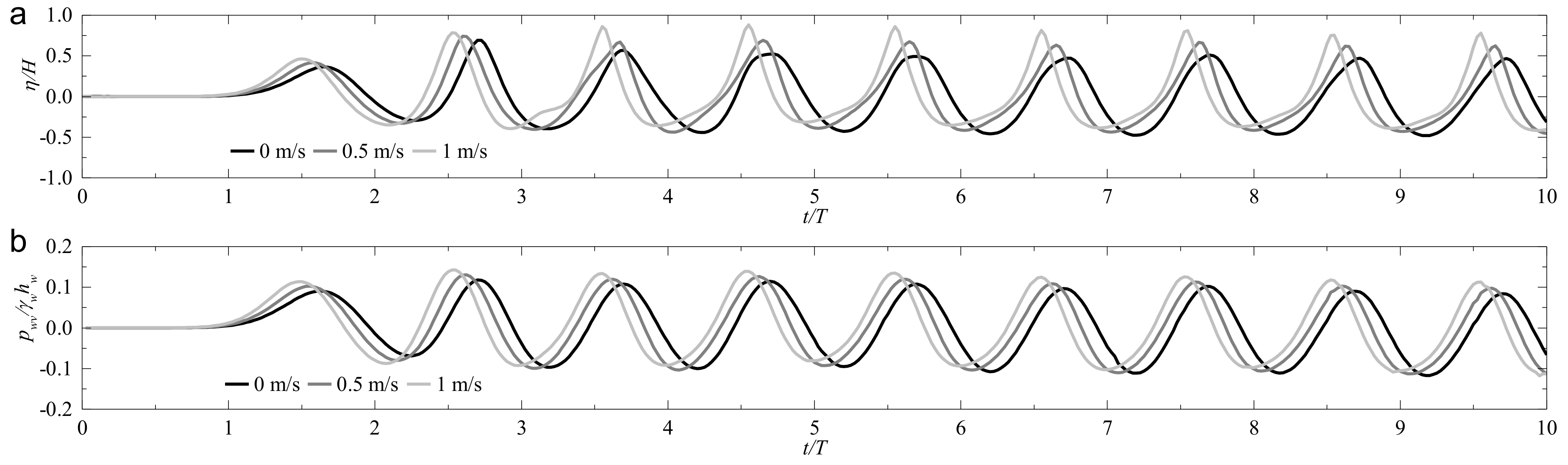
3.2. Hydrodynamics of WCSI

The previous studies on WCSI scarcely discussed the hydrodynamics of wave-current interaction as most of which directly use the analytical solution of Hsu et al. [10]. In this subsection, the free surface elevation and wave pressure on the seabed is shown and discussed. Among the previous studies, Zhang et al. [17] adopted the FVM-solved RANS equations with a $k$-$\epsilon$ turbulence closure scheme to simulate wave–current interactions with the internal wave-maker method. In the present study, based on the same governing equations, we adopted FDM to solve the problem with an incident wave generated at the inlet boundary.

Figure 4 displays the time series of free surface elevation and wave pressure on the seabed surface (location O is the midpoint on the seabed surface). It is seen that the current leads to a narrow steep crest and a flat trough of free surface elevation. As the current velocity goes up, the peak value of free surface elevation increases along with a decrease in the magnitude of the trough. Similar phenomena can also be found for the time development of wave pressure. It is known that the intensity of the wave and current-induced seabed liquefaction is dependent on the magnitude of negative wave pressure [5], i.e., negative wave pressure with larger magnitude leads to higher liquefaction potential. Therefore, it can be concluded that the existence and increase of current velocity would moderate the seabed liquefaction, which is in agreement with Zhang et al. [17]. However, this is in contrast to the result of those using the analytical solution of Hsu et al. [10] due to the assumption of uniform current omitting the effect of shear stress of the seabed. This demonstrates the necessity of considering the fluid viscosity and bed shear stress in WCSI.

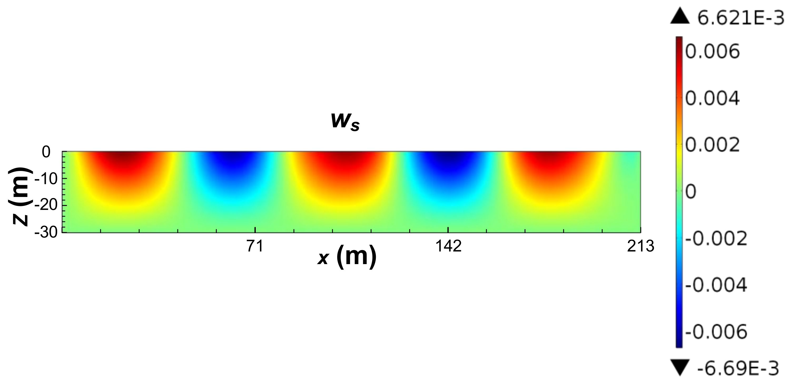
3.3. Seabed Response

Under the action of wave and current loading, excessive pore pressure will be generated in the seabed. It has been well recognized that the negative pore pressure is responsible for the wave-seabed liquefaction [4]. Correspondingly, the wave and current-induced seabed response, including the effective stresses, shear stress and pore pressure, will be presented in this subsection when the negative pore pressure reaches its maximum.

Figure 5 depicts the spatial distribution of wave and current-induced pore pressure ($p_s$) and displacements ($u_w, w_s$) when magnitude of negative wave pressure at the midpoint of seabed surface reaches its maximum ($t/T$ = 8.05) with current velocity of 0.5 m/s. As shown in the figure, seabed response to three waves is observed with an attenuation of magnitude from the inlet to the outlet. This is different from the result of Ye and Jeng [13] (Figure 6) due to the inclusion of fluid viscosity and bed friction in the present wave sub-model, which leads to the dissipation of wave energy during propagation. Besides, it is seen that the amplitude of the negative pore pressure in the horizontal plane is −12.21 kPa, which is 1.32 kPa larger than that of the positive pore pressure (10.89 kPa). Similar phenomenon is found in the distribution of vertical displacement. Ye and Jeng [13] have also shown similar phenomena in terms of pore pressure and vertical effective stress, using the analytical solution of wave–current interactions.

The effect of current velocity on seabed response has been extensively explored in the previous studies, and it is concluded that an increase of current velocity would intensify the seabed response within the analytical solution of Hsu et al. [10] on wave–current interactions. However, when the viscosity and turbulence are taken into account, Zhang et al. [18] revealed that the increase of current velocity would lead to reduction of the amplitude of pore pressure. In the present study, as shown in Figure 4, the amplitude of the positive wave pressure increases with the current velocity, while that of the negative wave pressure shows a converse trend, therefore this would lead to a different result on seabed response.

Figure 7 depicts the vertical distribution of wave and current-induced pore pressure ($p_s$), effective stresses (${\sigma }_x^{\prime },{\sigma }_z^{\prime }$) and shear stress (${\tau }_{xz}$) right beneath the midpoint (Figure 5a) when the magnitude of negative pore pressure reaches its maximum, in which $h$ is the thickness of the seabed. It can be observed that the magnitude of pore pressure drops down first and then increases slightly with the seabed depth, while the vertical effective stress (${\sigma }_z^{\prime }$) has a contrary trend. As for the horizontal effective stress (${\sigma }_x^{\prime }$) and shear stress, they both have a rather small magnitude throughout the seabed depth. Particularly, it can be seen that the existence and increase of current velocity lead to a decrease of the magnitude of pore pressure in the shallow seabed depth ($z/h$ < 0.3), as well as effective stresses and shear stress. In the deep soil range (z/h > 0.5), it could be observed that the increase in current velocity tends to decrease the magnitude of the seabed response. Particularly, there exists a slight increase of pore pressure when seabed depth $z/h$ increases from 0.7 to 1.0. This should be induced by the fixed impermeable bottom boundary, which restricts the seepage and soil displacements near the seabed bottom.

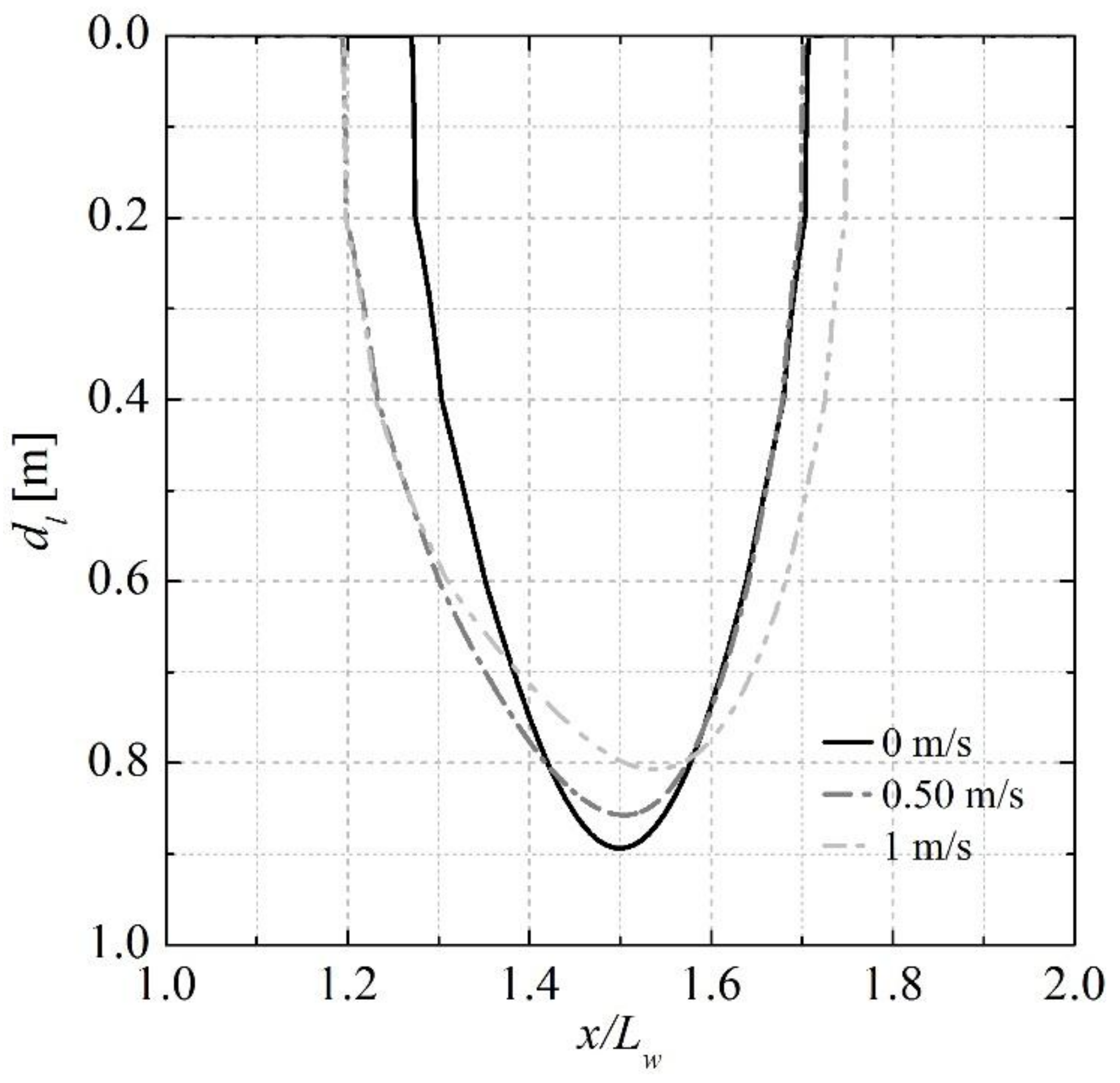
3.4. Seabed Liquefaction

There have been several liquefaction criteria proposed in the previous studies to estimate the liquefaction potential under wave (current) loadings. In the present study, the liquefaction criterion proposed by Zen and Yamazaki [42] is adopted to evaluate the liquefaction potential in seabed:

$$-\left({\gamma }_s-{\gamma }_w\right)z\le p_s-p_b$$

(18)

in which ${\gamma }_s$ is the unit weight of seabed soil and $p_b$ is the wave pressure on the seabed surface. In the previous studies, this liquefaction criterion has been widely adopted to estimate the wave-induced seabed liquefaction potential around pipelines [43,44], breakwaters [45] and pile foundations [38,39,46]. In this study, the soil unit weight is taken as $1.8{\gamma }_w$.

Figure 8 illustrates the seabed liquefaction depth ($d_l$) when the magnitude of negative wave and current-induced pore pressure reaches its maximum. It is seen that the maximum liquefaction depth reaches nearly 0.9 m when current velocity is zero. When there is a current, it can be seen that the liquefaction depth displays a decrease, however, with an increase in width of the liquefaction area. This corresponds to the elongation effect of current on wave trough as illustrated in Figure 4.

Figure 9 presents the variations of maximum liquefaction depth ($d_l$) and width ($w_l$) with current velocity ($v_c$). It is shown that with the increase of current velocity from 0 to 1.0 m/s, the liquefaction depth drops down. However, the width of the liquefaction area increases with the increase of current velocity.

4. Discussion

The CFD method is used in the present study to generate waves and simulate the wave–current interactions, and the RANS equations with $k$-$\epsilon$ turbulence model are taken as the governing equations with the VOF method to describe the free surface motion. Thus, the viscosity and turbulence of wave and current motion could be enclosed in this study in comparison with the analytical approximation of Hsu et al. [10] which simplified the fluid motion as inviscid and irrotational potential flow. Based on these governing equations, Zhang et al. [17,18,19] took FVM to solve the wave–current interactions with the internal wave maker method, in which sponge layers are set at both ends of the numerical flume to eliminate the wave reflection. In the present study, the FDM method is used to solve the governing equations rather than FVM. The inlet velocity method is used to generate the wave train and current with only one sponge layer at the outflow boundary. Thus, computation time and memory consumption could be saved in the present study in comparison with the model of Zhang et al. [17,18,19].

Based on the analytical approximation of Hsu et al. [10], the previous studies found that the increase of current velocity would aggravate the seabed liquefaction depth. However, when the RANS equations with $k$-$\epsilon$ turbulence model are taken to calculate the wave loading, a contrary trend is found, both in Zhang et al. [18] and the present study (Figure 6 and Figure 7). In Hsu et al. [10], potential flow theory is adopted and the current is considered to be uniform. Hence, it goes against the fact that the current velocity near the seafloor should be quite small, even negligible due to the non-slip boundary. Correspondingly, the CFD method (RANS equations with $k$-$\epsilon$ turbulence model) is more reasonable when simulating wave-current interaction.

5. Conclusions

The oscillatory seabed response to combined wave and current loading is numerically explored in this paper. The FDM-solved RANS equations with $k$-$\epsilon$ turbulence closure and velocity-inlet wave maker are employed to simulate the wave–current interactions. Biot’s QS model for a poro-elastic medium is adopted to govern the seabed response. The conclusions could be drawn as follows:

(1) The existence of current elongates the wave trough and meanwhile leads to a short wave crest. The wave energy attenuates with wave propagation, leading to magnitude attenuation of seabed response.

(2) The increase of current velocity intensifies the positive wave pressure on the seabed surface, and moderates the negative wave pressure. In the shallow seabed, the seabed response is alleviated with the current velocity while it intensifies in the deep soil range.

(3) The seabed liquefaction depth decreases with the current velocity, while the width of the liquefaction zone increases with the current velocity. This corresponds to the effect of current velocity on wave profile and wave pressure.

References

1. Sterling, G.H.; Strohbeck, G.E. The Failure of the south pass 70 platform B in Hurricane Camille. J. Pet. Technol. 1975, 27, 263–268. [Google Scholar] [CrossRef]
2. Smith, A.W.S.; Gordon, A.D. Large breakwater toe failures. J. Waterw. Pt. Coast. Ocean Eng. 1983, 109, 253–255. [Google Scholar] [CrossRef]
3. Franco, L. Vertical breakwaters: the Italian experience. Coast. Eng. 1994, 22, 31–55. [Google Scholar] [CrossRef]
4. Jeng, D.S. Wave-induced sea floor dynamics. Appl. Mech. Rev. 2003, 56, 407–429. [Google Scholar] [CrossRef]
5. Sumer, B.M. Liquefaction around Marine Structures; Liu, P.L.F., Ed.; World Scientific: Singapore, 2014. [Google Scholar]
6. Huang, Y.; Bao, Y.; Zhang, M.; Liu, C.; Lu, P. Analysis of the mechanism of seabed liquefaction induced by waves and related seabed protection. Nat. Hazards 2015, 79, 1399–1408. [Google Scholar] [CrossRef]
7. Zhang, J.; Li, Q.; Ding, C.; Zheng, J.; Zhang, T. Experimental investigation of wave-driven pore-water pressure and wave attenuation in a sandy seabed. Adv. Mech. Eng. 2016, 8, 1–10. [Google Scholar] [CrossRef]
8. Liao, C.; Tong, D.; Jeng, D.-S.; Zhao, H. Numerical study for wave-induced oscillatory pore pressures and liquefaction around impermeable slope breakwater heads. Ocean Eng. 2018, 157, 364–375. [Google Scholar] [CrossRef]
9. Liao, C.; Tong, D.; Chen, L.H. Pore pressure distribution and momentary liquefaction in vicinity of impermeable slope-type breakwater head. Appl. Ocean Res. 2018, 78, 290–306. [Google Scholar]
10. Hsu, H.C.; Chen, Y.Y.; Hsu, J.R.C.; Tseng, W.J.; Hsu, H.C.; Chen, Y.Y.; Hsu, J.R.C.; Tseng, W.J. Nonlinear water waves on uniform current in Lagrangian coordinates. J. Nonlinear Math. Phys. 2009, 16, 47–61. [Google Scholar] [CrossRef]
11. Ulker, M.B.C.; Rahman, M.S.; Jeng, D.S. Wave-induced response of seabed: various formulations and their applicability. Appl. Ocean Res. 2009, 31, 12–24. [Google Scholar] [CrossRef]
12. Cheng, A.H.D.; Liu, P.L.F. Seepage force on a pipeline buried in a poroelastic seabed under wave loadings. Appl. Ocean Res. 1986, 8, 22–32. [Google Scholar] [CrossRef]
13. Ye, J.H.; Jeng, D.S. Response of porous seabed to nature loadings: Waves and currents. J. Eng. Mech. 2012, 138, 601–613. [Google Scholar] [CrossRef]
14. Zienkiewicz, O.C.; Chang, C.T.; Bettess, P. Drained, undrained, consolidating and dynamic behaviour assumptions in soils. Géotechnique 1980, 30, 385–395. [Google Scholar] [CrossRef]
15. Alfonsi, G.; Lauria, A.; Primavera, L. Recent results from analysis of flow structures and energy modes induced by viscous wave around a surface-piercing cylinder. Math. Probl. Eng. 2017, 2017, 1–10. [Google Scholar] [CrossRef]
16. Alfonsi, G.; Lauria, A.; Primavera, L. Proper orthogonal flow modes in the viscous-fluid wave-diffraction case. J. Flow Vis. Image Process. 2013, 20, 227–241. [Google Scholar] [CrossRef]
17. Zhang, J.S.; Zhang, Y.; Jeng, D.S.; Liu, P.L.F.; Zhang, C. Numerical simulation of wave-current interaction using a RANS solver. Ocean Eng. 2014, 75, 157–164. [Google Scholar] [CrossRef]
18. Zhang, J.S.; Zhang, Y.; Zhang, C.; Jeng, D.S. Numerical modeling of seabed response to combined wave-current loading. J. Offshore Mech. Arct. Eng. 2013, 135, 125–131. [Google Scholar] [CrossRef]
19. Zhang, J.; Zheng, J.; Jeng, D.S.; Guo, Y. Numerical simulation of solitary-wave propagation over a steady current. J. Waterw. Port Coastal Ocean Eng. 2015, 141, 04014041. [Google Scholar] [CrossRef]
20. Lin, P.; Liu, P.L.-F. Internal wave-maker for navier-stokes equations models. J. Waterw. Port Coast. Ocean Eng. 1999, 125, 207–215. [Google Scholar] [CrossRef]
21. Wen, F.; Wang, J.H. Response of Layered Seabed under Wave and Current Loading. J. Coast. Res. 2015, 314, 907–919. [Google Scholar] [CrossRef]
22. Wen, F.; Wang, J.H.; Zhou, X.L. Response of saturated porous seabed under combined short-crested waves and current loading. J. Coast. Res. 2016, 318, 286–300. [Google Scholar] [CrossRef]
23. Zhang, X.; Zhang, G.; Xu, C. Stability analysis on a porous seabed under wave and current loadings. Mar. Georesources Geotechnol. 2017, 35, 710–718. [Google Scholar] [CrossRef]
24. Biot, M.A. Mechanics of deformation and acoustic propagation in porous media. J. Appl. Phys. 1962, 33, 1482–1498. [Google Scholar] [CrossRef]
25. Yang, G.; Ye, J. Wave & current-induced progressive liquefaction in loosely deposited seabed. Ocean Eng. 2017, 142, 303–314. [Google Scholar]
26. Ye, J.; Jeng, D.; Wang, R.; Zhu, C. Validation of a 2-D semi-coupled numerical model for fluid-structure-seabed interaction. J. Fluids Struct. 2013, 42, 333–357. [Google Scholar] [CrossRef]
27. Zhang, Y.; Jeng, D.S.; Gao, F.P.; Zhang, J.S. An analytical solution for response of a porous seabed to combined wave and current loading. Ocean Eng. 2013, 57, 240–247. [Google Scholar] [CrossRef] [Green Version]
28. Biot, M.A. General theory of three-dimensional consolidation. J. Appl. Phys. 1941, 12, 155–164. [Google Scholar] [CrossRef]
29. Liu, B.; Jeng, D.S.; Zhang, J.S. Dynamic response in a porous seabed of finite depth to combined wave and current loadings. J. Coast. Res. 2014, 296, 765–776. [Google Scholar] [CrossRef]
30. Liao, C.C.; Jeng, D.S.; Zhang, L.L. An analytical approximation for dynamic soil response of a porous seabed due to combined wave and current loading. J. Coast. Res. 2015, 315, 1120–1128. [Google Scholar] [CrossRef]
31. Hirt, C.W.; Nichols, B.D. Volume of fluid (VOF) method for the dynamics of free boundaries. J. Comput. Phys. 1981, 39, 201–225. [Google Scholar] [CrossRef]
32. Lin, P.; Liu, P.L.F. A numerical study of breaking waves in the surf zone. J. Fluid Mech. 1998, 359, 239–264. [Google Scholar] [CrossRef]
33. Orlanski, I. A simple boundary condition for unbounded hyperbolic flows. J. Comput. Phys. 1976, 21, 251–269. [Google Scholar] [CrossRef]
34. Jeng, D.S. Porous Models for Wave-seabed Interactions; Springer: Berlin/Heidelberg, Germany, 2013. [Google Scholar]
35. Tsui, Y.; Helfrich, S.C. Wave-induced pore pressures in submerged sand layer. J. Geotech. Eng. 1983, 109, 603–618. [Google Scholar] [CrossRef]
36. Liu, B.; Jeng, D.-S.; Ye, G.L.; Yang, B. Laboratory study for pore pressures in sandy deposit under wave loading. Ocean Eng. 2015, 106, 207–219. [Google Scholar] [CrossRef]
37. Hsu, J.R.C.; Jeng, D.S. Wave-induced soil response in an unsaturated anisotropic seabed of finite thickness. Int. J. Numer. Anal. Methods Geomech. 1994, 18, 785–807. [Google Scholar] [CrossRef]
38. Tong, D.; Liao, C.; Jeng, D.S.; Zhang, L.; Wang, J.; Chen, L. Three-dimensional modeling of wave-structure-seabed interaction around twin-pile group. Ocean Eng. 2017, 145, 416–429. [Google Scholar] [CrossRef]
39. Tong, D.; Liao, C.; Jeng, D.; Wang, J. Numerical study of pile group effect on wave-induced seabed response. Appl. Ocean Res. 2018, 76, 148–158. [Google Scholar] [CrossRef]
40. Tong, D.; Liao, C.; Wang, J.; Jeng, D. Wave-induced oscillatory soil response around circular rubble-mound breakwater head. In Proceedings of the International Conference on Ocean, Offshore and Arctic Engineering, Trondheim, Norway, 25–30 June 2017; Volume 155, pp. V009T10A008. [Google Scholar]
41. Umeyama, M. Coupled PIV and PTV measurements of particle velocities and trajectories for surface waves following a steady current. J. Waterw. Port Coastal Ocean Eng. 2011, 137, 85–94. [Google Scholar] [CrossRef]
42. Zen, K.; Yamazaki, H. Mechanism of wave-induced liquefaction and densification in seabed. SOILS Found. 1990, 30, 90–104. [Google Scholar] [CrossRef]
43. Lin, Z.; Guo, Y.; Jeng, D.; Liao, C.; Rey, N. An integrated numerical model for wave-soil-pipeline interactions. Coast. Eng. 2016, 108, 25–35. [Google Scholar] [CrossRef]
44. Zhou, X.L.; Zhang, J.; Guo, J.J.; Wang, J.H.; Jeng, D.S. Cnoidal wave induced seabed response around a buried pipeline. Ocean Eng. 2015, 101, 118–130. [Google Scholar] [CrossRef]
45. Jeng, D.-S.; Ou, J. 3D models for wave-induced pore pressures near breakwater heads. Acta Mech. 2010, 215, 85–104. [Google Scholar] [CrossRef]
46. Lin, Z.; Pokrajac, D.; Guo, Y.; Jeng, D.S.; Tang, T.; Rey, N.; Zheng, J.; Zhang, J. Investigation of nonlinear wave-induced seabed response around mono-pile foundation. Coast. Eng. 2017, 121, 197–211. [Google Scholar] [CrossRef] [Green Version]
Figure 1. Definition of wave–current–seabed interactions.
Jmse 06 00088 g001
Figure 2. Validation of time series of pore pressure against experiment data of Liu et al. [36] at depths (a) z = −6.7 cm and (b) z = −26.7 cm (Adapted from Tong et al. [38]).
Jmse 06 00088 g002
Figure 3. Validation of the fluid sub-model against the experiment data of Umeyama [41].
Jmse 06 00088 g003
Figure 4. Time series of (a) free surface elevation and (b) wave pressure at location O for various current velocities.
Jmse 06 00088 g004
Figure 5. Seabed response to combined wave and current loading when current velocity vc = 0.5 m/s.
Jmse 06 00088 g005aJmse 06 00088 g005b
Figure 6. Seabed response to combined wave and current loading when v c = 1   m / s in Ye and Jeng [13].
Jmse 06 00088 g006
Figure 7. Vertical distributions of minimum wave-induced pore pressure with various current velocities.
Jmse 06 00088 g007
Figure 8. Maximum liquefaction depth with various current velocities.
Jmse 06 00088 g008
Figure 9. Maximum liquefaction depth and width around location O with various current velocities.
Jmse 06 00088 g009