Article

Simulation of the Arctic—North Atlantic Ocean Circulation with a Two-Equation K-Omega Turbulence Parameterization

by
Sergey Moshonkin
1,2,†,
Vladimir Zalesny
1,2,† and
Anatoly Gusev
1,2,3,*,†
1
Marchuk Institute of Numerical Mathematics of the Russian Academy of Sciences, Moscow, Russia
2
Marine Hydrophysical Institute of the Russian Academy of Sciences, Sevastopol, Russia
3
P.P. Shirshov Institute of Oceanology of the Russian Academy of Sciences, Moscow, Russia
*
Author to whom correspondence should be addressed.
Current address: Gubkina st., 8. 119333 Moscow, Russian.
J. Mar. Sci. Eng. 2018, 6(3), 95; https://doi.org/10.3390/jmse6030095
Submission received: 27 April 2018 / Revised: 7 August 2018 / Accepted: 17 August 2018 / Published: 18 August 2018

Abstract

:
The results of large-scale ocean dynamics simulation taking into account the parameterization of vertical turbulent exchange are considered. Numerical experiments were carried out using k ω turbulence model embedded to the Institute of Numerical Mathematics Ocean general circulation Model (INMOM). Both the circulation and turbulence models are solved using the splitting method with respect to physical processes. We split k ω equations into the two stages describing transport-diffusion and generation-dissipation processes. At the generation-dissipation stage, the equation for ω does not depend on k. It allows us to solve both turbulence equations analytically that ensure high computational efficiency. The coupled model is used to simulate the hydrophysical fields of the North Atlantic and Arctic Oceans for 1948–2009. The model has a horizontal resolution of 0.25 and 40 σ -levels along the vertical. The numerical results show the model’s satisfactory performance in simulating large-scale ocean circulation and upper layer dynamics. The sensitivity of the solution to the change in the coefficients entering into the analytical solution of the k ω model which describe the influence of some physical factors is studied. These factors are the climatic annual mean buoyancy frequency (AMBF) and Prandtl number as a function of the Richardson number. The experiments demonstrate that taking into account the AMBF improves the reproduction of large-scale ocean characteristics. Prandtl number variations improve the upper mixed layer depth simulation.
PACS:
92.10.ab; 02.60.Cb; 92.10.Lq; 02.70.Bf

1. Introduction

The simulation of momentum, heat and salt vertical turbulent exchange is very important for ocean general circulation models (OGCMs). In OGCMs, vertical mixing is parameterized using a second-order differential operator with variable exchange coefficients K U , K T and K S [1,2,3,4,5]. The two basic approaches are used to determine these coefficients: (1) they are defined as functions of stratification and velocity shift or the local Richardson number [1,6,7,8]; (2) they can be found using additional turbulence models [3,9,10,11,12,13,14,15]. The first approach is more simple and efficient from the computational point of view. This approach is traditionally used in numerical simulation of large-scale ocean circulation [6]. The second one gives better results from the physical point of view [15], however, the computation cost increases. Therefore, when using the second approach, special attention should be paid to the construction of an effective numerical technique for solving turbulence equations.
To simulate large-scale ocean circulation we use the traditional Reynolds averaged equations with parameterized vertical turbulent fluxes u w ¯ , v w ¯ , T w ¯ , S w ¯ , where u , v , w , T and S are turbulent disturbances for the velocity components, temperature and salinity. With the framework of K-hypothesis, the turbulent fluxes are related to the local gradients of the corresponding mean quantities by eddy viscosities and diffusivities. With this parameterization, the turbulent coefficients depend on the both turbulence characteristics and the stability functions, which are also derived from the equations for turbulent fluxes [15,16,17,18].
The turbulence models used for parameterization of turbulent viscosity and diffusivity in OGCMs are based on the equations for the turbulent kinetic energy (TKE) and the characteristic needed for closure of the system. Such characteristics may be following ones: ϵ is specific dissipation rate of TKE by the water viscosity; ω is frequency characteristic of the turbulence decay process [19] or, briefly, the turbulent dissipation frequency (TDF); and l is turbulence spatial scale. The corresponding two-equation turbulence models or closure schemes are referred to as k ϵ , k ω and k k l . In respect to formulation, they are similar and can be combined as a “generalized scale method” [15,20]. The characteristics ϵ , ω and l are connected by algebraic relations, including the TKE k and the stability function for neutral stratification c S 0 : ϵ = ( c S 0 ) 3 k 3 / 2 l , ω = ϵ ( c S 0 ) 4 k , l = k 3 / 2 c S 0 ω [17,19]. The k k l Mellor-Yamada level 2.5 model (MY) [13,21,22] and its modifications [16,23] are most used for parameterization of turbulent viscosity and diffusivity in OGCMs [13,15]. Usage of the k ϵ and k ω models for the parameterization of K U , K T and K S in OGCMs has some specific features [9,24].
The new closure for definition of K U , K T and K S on the basis of Reynolds stress equations is proposed in [25]. The coefficients are defined for developed turbulence, low turbulence in the pycnocline, and in the bottom turbulence zone. In this parameterization [25], the two-equation turbulence model k ϵ is used to compute dissipation in the developed turbulence zone as well.
In our research, we couple an OGCM with the k ω turbulence model [9,11]. Our choice is mainly justified by the mathematical advantage of the latter. Novelty consists in applying the splitting technique for solving the k ω equations [5,26]. We split k ω equations into the two main stages describing transport-diffusion and generation-dissipation processes. At the generation-dissipation stage, the equation for ω does not depend on k. It allows us to solve (at this stage) the k ω equations analytically that ensures high computational efficiency.
The splitting algorithms with respect to physical processes and spatial coordinates are applied in the both turbulence model and INMOM. It allowed to make the approach to the mixing parameterization with using the k ω model more convenient. The aims of the paper are as follows:
  • to present a new splitting algorithm for solving k ω turbulence equations that allows to reduce the complete system to the stages of transport-diffusion and generation-dissipation;
  • to find an analytical solution of k ω equations at the generation-dissipation splitting stage that is impossible for k k l and k ϵ closures;
  • to demonstrate possibilities of controlling the obtained analytical solution of k ω equations through its coefficients by means of different physical factors. We take into account such physical factors as climatic annual mean buoyancy frequency (AMBF) and Prandtl number as function of the Richardson number to goal this aim;
  • to compare results of numerical experiments with the INMOM + ( k ω ) to data on the hydrographic structure of the North Atlantic and Arctic Ocean to demonstrate physical effects of the accounting AMBF and variations of the Prandtl number.

2. Model and Methods

2.1. Equations of the Ocean General Circulation Model

The INMOM is based on a primitive equation system written in a generalized orthogonal coordinates on sphere under incompressibility, hydrostatics, and Boussinesq approximations [5,27]. The vertical coordinate is dimensionless variable σ [ 0 , 1 ] :
σ = z ζ H ζ ,
where z is the usual vertical coordinate directed downward, H is the ocean depth, and ζ is the sea surface height, which is positive when under the undisturbed surface. Model equations written in symmetrized form are [5]:
D t u Z σ f + η v = Z σ ρ 0 r x x p g 2 Z ρ g 2 ρ Z x Z ρ x + 1 Z σ σ K U u σ + D u u ,
D t v + Z σ f + η u = Z σ ρ 0 r y y p g 2 Z ρ g 2 ρ Z y Z ρ y + 1 Z σ σ K U v σ + D v v ,
σ p g 2 Z ρ = g 2 ρ Z σ Z ρ σ ,
ζ t + 1 r x r y x Z σ r y u + y Z σ r x v + w σ σ = 0 ,
D t T = 1 Z σ σ K T T σ + D T T R σ ,
D t S = 1 Z σ σ K S S σ + D S S ,
ρ = ρ T , S , p ^ ρ ˜ T + T ¯ , S + S ¯ , p ^ ρ ˜ T ¯ , S ¯ , p ^ .
Here, x and y are generalized orthogonal coordinates in horizontal subspace; r x and r y are metric coefficients, in spherical coordinates computes as: r x = R E cos y , r y = R E , R E is the Earth radius; Z = ( H ζ ) σ + ζ , Z σ = H ζ , Z x Z x , Z y Z y :
f = 2 Ω ˜ sin φ , η = 1 r x r y r y x v r x y u ,
l is the Coriolis parameter, φ is geographical latitude and Ω ˜ is the Earth angular velocity. D t is the transport operator written in symmetrized form:
D t ψ D t u ψ = 1 2 Z σ ψ t + Z σ ψ t + 1 2 r x r y x Z σ r y u ψ + Z σ r y u ψ x + y Z σ r x v ψ + Z σ r x v ψ y + 1 2 σ w σ ψ + w σ ψ σ ,
where ψ is transported variable, u = u , v , w σ is the velocity vector in the σ -coordinate system; w σ is the vertical velocity in the σ -coordinate system defined as
w σ = w 1 σ ζ t + u r x Z x + v r y Z y ,
T and S are deviations of potential temperature and salinity from their means T ¯ , S ¯ ; p ^ = ρ 0 g Z is an approximate function of hydrostatic pressure; R is the penetrative solar radiation flux; ρ is the density computed according to [28]; and K U , K T and K S are the coefficients of vertical turbulent viscosity and diffusivity.
The operators D T , D S describing lateral mixing of heat and salt along isopycnal surfaces are D T = D S D ϕ :
D ψ ψ = 1 r x r y x μ Z σ r y r x ψ x ρ x ρ σ ψ σ 1 r x r y σ μ Z σ r y r x ρ x ρ σ ψ x ρ x ρ σ ψ σ + 1 r x r y y μ Z σ r x r y ψ y ρ y ρ σ ψ σ 1 r x r y σ μ Z σ r x r y ρ y ρ σ ψ y ρ y ρ σ ψ σ ,
where ψ is diffused variable, μ is lateral diffusion coefficient, ρ x ρ p o t x , ρ y ρ p o t y , ρ σ ρ p o t σ . Turbulent viscosity operators D u , D v are a combination of laplacian and biharmonic operators in plain form performing mixing along σ -surfaces [5].
Model includes interactive module which describes sea ice dynamics and thermodynamics [29].

2.2. The Two-Equation K-Omega Turbulence Model

The OGCM was subsequently coupled with the two-equation k ω turbulence model. This model involves the solution of evolutionary equations for the turbulent kinetic energy k (TKE) and the turbulence dissipation frequency ω (TDF) [15,19]. The coefficients of turbulent viscosity K U and turbulent diffusivities for heat K T and salt K S are given as functions of TKE and TDF:
K U = C S U c S 0 k ω .
Here C S U is the dimensionless stability function, c S 0 = 0.5562 is its value for neutral stratification [15]; k = 0.5 u u + v v + w w ¯ is TKE, the bar above denotes averaging over the ensemble (or time), and the values with strokes are turbulent pulsations relative to the mean flow u = u , v , w ; ω = ϵ ( c S 0 ) 4 k is TDF, ϵ is rate of TKE transformation to internal thermal energy of water due to dissipation.
For the temperature turbulent diffusivity, K T = C S T c S 0 k ω . Suppose that C S U = c S 0 and C S T = C S U Pr in the elementary σ -layer, where Pr is Prandtl number (see, e.g., equations (2.73)–(2.74) from [30]). As well, suppose that K S = K T for fully developed turbulent flows. As a result, we use the following dependencies: K S = K T = K U Pr .
The standard two-equation k ω turbulence model is [15,19]:
D t k = 1 Z σ σ K U σ k k σ + D k k + Z σ K U G 2 K ρ N 2 ( c S 0 ) 4 ω k ,
D t ω = 1 Z σ σ K U σ ω ω σ + D ω ω + Z σ ω k c 1 ω K U G 2 c 3 ω K ρ N 2 c 2 ω ( c S 0 ) 4 k ω .
Here G 2 = 1 Z σ u σ 2 + 1 Z σ v σ 2 and N 2 = g ρ 0 1 Z σ ρ σ are the velocity shift and buoyancy frequency in the second degree ( N 2 > 0 corresponds to stable stratification), D k and D ω are mixing operators computed by the Equation (12).
Note: relations (14)–(15) are used only in layers where the developed turbulence presents and k > 0.03 cm 2 / s 2 [30]. Otherwise, small background values of exchange coefficients (intermittent turbulence) K U m i n = 1.0 and K T m i n = 0.05 cm 2 /s are used.

2.3. Boundary and Initial Conditions

Boundary conditions for (2)–(8), (14) and (15) are as follows. At the sea free surface σ = 0 :
K U Z σ u σ = τ a x ρ 0 , K U Z σ v σ = τ a y ρ 0 , w σ = 0 , K T Z σ T σ + α T T T o b s = q T , K S Z σ S σ + α S S S o b s = q S , K U Z σ σ k k σ = C g u S 3 , K U Z σ σ ω ω σ = 0 ,
where τ a x , τ a y are the wind stress components, α T , α S are the relaxation coefficients, q T and q S are the total heat and salt fluxes, C g is wind generation parameter [13,31,32], u S = τ a x 2 + τ a y 2 ρ 0 1 / 2 is friction velocity in the upper ocean layer.
At the sea bottom σ = 1 :
K U Z σ u σ = τ b x ρ 0 , K U Z σ v σ = τ b y ρ 0 , w σ = 0 , K T Z σ T σ = 0 , K S Z σ S σ = 0 , K U Z σ σ k k σ = C g u B 3 , K U Z σ σ ω ω σ = 0 ,
where τ b x = ρ 0 C D u 2 + v 2 + e b 2 u and τ b y = ρ 0 C D u 2 + v 2 + e b 2 v are bottom stress components, C D = 2.5 × 10 3 , e b = 5 cm/s are empirical constants, u B = τ b x 2 + τ b y 2 ρ 0 1 / 2 is friction velocity in the bottom ocean layer.
Thus, at the top and bottom surfaces we apply the corresponding boundary conditions for momentum, heat and salt fluxes, turbulent kinetic energy, and dissipation frequency [7,9]. At the lateral boundary, normal velocity, normal derivative of tangent velocity, heat, salt, turbulent kinetic energy and dissipation frequency fluxes are assumed to be equal to zero. The corresponding initial conditions for u, v, ζ , T, S, k and ω are specified at t = 0 .

2.4. Numerical Algorithm

The numerical solution of the OGCM + k ω model is based on the splitting method applying for evolutionary equations [33]. We formulate the system of governing equations in evolutionary form and represent the operator of the differential problem as a sum of more simple nonnegative suboperators. Just for this purpose it is convenient to use σ -coordinate system [5,27]. It allows us (1) to transform 3D computational domain to 3D volume with unity depth; (2) to exclude time derivative from boundary condition at the sea surface ( w = d ζ d t for z-coordinates); (3) to represent transport operator in convenient nonnegative form acting on D ( x , y ) × [ 0 , 1 ] ; (4) rewrite, finally, both OGCM and turbulence model operators in evolutionary form. The key points of the approach proposed are as follows. When using the splitting method the form of a differential problem is of great importance. The most convenient form of equations is their symmetrized form. By the symmetrized form we mean the form of equations, which satisfies the conditions:
  • The symmetrized form gives the form of the adjoint operator, which is close to the original one.
  • This form leads to the finite difference approximation retaining the main properties typical of original differential operators (symmetry, skew-symmetry, nonnegativeness).
  • From the form naturally follows the splitting of the problem operator into the sum of simple nonnegative operators.
Formulation Equations (2)–(8), (14) and (15) in symmetrized form makes it possible to use the splitting algorithm with respect physical processes and spatial coordinates x, y and σ [27,33]. The equations for u, v, T, S, ζ at each time interval t j < t < t j + 1 are split with respect to physical processes into two macro-stages: transport-diffusion of u, v, T, S:
D t u Z σ η v = 1 Z σ σ K U u σ + D u u ,
D t v + Z σ η u = 1 Z σ σ K U v σ + D v v ,
D t T = 1 Z σ σ K T T σ + D T T R σ ,
D t S = 1 Z σ σ K S S σ + D S S ,
and the adaptation of velocity and density fields:
u t f v = 1 ρ 0 r x x p g 2 Z ρ g 2 ρ Z x Z ρ x ,
v t + f u = 1 ρ 0 r y y p g 2 Z ρ g 2 ρ Z y Z ρ y ,
σ p g 2 Z ρ = g 2 ρ Z σ Z ρ σ ,
ζ t + 1 r x r y x Z σ r y u + y Z σ r x v + w σ σ = 0 ,
If needed, within the transport-diffusion macro-stage the equations can be secondary split with respect to separate coordinates x, y and σ . At the adaptation macro-stage, a representation
u = u ¯ + u , v = v ¯ + v , u ¯ = 0 1 u d σ , v ¯ = 0 1 v d σ
is used and implicit time scheme for the treatment of the depth averaged velocities and sea surface height ζ (linear shallow water equations) is applied. With respect to spatial coordinates, staggered grid [34], known in meteorology as “C”-grid [35], is used. Note, that the numerical algorithm for the solution of (2)–(8) is described in more detail in [5,27].
To solve (14) and (15) on the time interval t j < t < t j + 1 we assume that three velocity components in the left-hand side of (14) and (15) are known. Splitting of turbulence Equations (14) and (15) is performed in terms of physical processes into two stages. At the first splitting stage we solve three-dimensional transport-diffusion equations:
D t k = 1 Z σ σ K U σ k k σ + D k k ,
D t ω = 1 Z σ σ K U σ ω ω σ + D ω ω ,
with initial conditions k = k j , ω = ω j at t = t j . Note that within the transport-diffusion stage the equations can be secondary split with respect to separate coordinates x, y and σ [5,26,33]. As a result we have k j + 1 k ( t j + 1 ) , ω j + 1 ω ( t j + 1 ) .
At the second splitting stage, on the same time interval t j < t < t j + 1 , we solve equations describing the generation-dissipation process [9,10,11]:
ω t = B C ω 2 ,
k t = A ω D ω k .
with initial conditions equal to the solution of the first splitting stage: k = k j + 1 , ω = ω j + 1 at t = t j .
Here we can write separately the coefficients A, B, C and D for (29) and (30), using both the stability function for diffusivity C S ρ = C S T , and the Prandtl number Pr:
A = 1 c S 0 C S U G 2 C S ρ N 2 = C S U c S 0 G 2 1 Pr N 2 ,
B = 1 c S 0 c 1 ω C S U G 2 c 3 ω C S ρ N 2 = C S U c S 0 c 1 ω G 2 c 3 ω Pr N 2 ,
C = c 2 ω c S 0 4 , D = c S 0 4 .
Note that B > 0 , C > 0 and D > 0 while A can change the sign. On the interval t j < t < t j + 1 during the calculating k and ω , variables N 2 and G 2 do not vary with respect to time.
As an example, we choose the coefficients A and B as functions of the Prandtl number. The latter is a function of N 2 and G 2 (see further) rather than a function of time at the interval t j < t < t j + 1 . Stability function for momentum is chosen as a constant C S U = c S 0 (see, e.g., Equation (2.73) from [30]). In this case, the system (29) and (30) has a clear analytical solution at the time step of the circulation model. The analytical solution is available for k ω model because at the generation-dissipation stage equation for ω does not depend upon k. The analytical solution of (29) and (30) has the form:
ω = r d ( r m + r p a r ) / ( r m r p a r ) , k = k 0 E 1 E 2 A 2 B E 3 E 4 D 2 C ,
where
r d = B / C , r m = ω 0 r d , r p = ω 0 + r d , a r = exp 2 B C · t , E 1 = ( r m + r p a r ) 2 , E 2 = 4 ( ω 0 ) 2 a r , E 3 = 4 r d 2 a r , E 4 = ( r m r p a r ) 2 .
We refer to the algorithm using the analytic solution (34) as the “splitting turbulence algorithm” (STA).
It follows from (34) that ω B / C for t [9]. The expression ω = B / C is the asymptotic of the solution (34). Using it, we can also find the asymptotic behavior of the TKE. Then the asymptotic solution of (29) and (30) has the form:
ω = B / C , k = k 0 exp γ t ,
where γ = A ω D ω = A C B D B C .

3. Scenarios of Numerical Experiments

A set of experiments EX1–EX4 is performed as summarized in Table 1. The model equations are written in a spherical coordinate system. The poles are located on the geographical equator at 120 W and 60 E. The simulation domain includes the Atlantic Ocean north of 30 S, Arctic Ocean and Bering Sea. Open boundaries of the area pass through 30 S and the straits of the Aleutian Islands. As well, the domain includes the Mediterranean, Black and Baltic Seas. The grid spacing in latitude and longitude is 0.25 . 40 σ -levels are set along the vertical with refinement near the ocean surface. The bottom topography is taken from [36]. The data were smoothed in accordance with the horizontal resolution of the model so that there are no strong bottom gradients. The model is forced at the sea surface with the CORE historical atmospheric datasets for the period 1948–2009 [37].
The initial conditions are climatic average January temperature and salinity fields taken from [38], no motion, and no sea ice. All the experiments were performed for the period 1948–2009. The OGCM equations are solved with a time step τ o c m = 1 h. At the transport-diffusion splitting stage the k ω equations are solved with the same time step τ o c m = 1 h. At the generation-dissipation stage, in experiments EX1–EX3, an analytical solution is used with time step τ T = 5 min for secondary splitting with using fractional step method. Note that coefficients A and B in the analytical solution depend on Prandtl number and AMBF.
Basic experiment EX1. In the EX1, in coefficients A and B we put Pr = 1 , and for turbulent exchange coefficients, Pr is calculated according to [39] in the form:
Pr = 1 , R i 0.2 5 R i , 0.2 < R i < 2 10 , R i 2 .
Here, the functions N 2 , G 2 , R i = N 2 G 2 , Pr are constant at the interval t j < t < t j + 1 . The parameterization (36) proposed in [39] is currently used to define turbulent diffusivity in the OGCM (see, e.g., [23]). As well, the articles appeared where Pr is computed as a function of buoyancy frequency and turbulent characteristics [12,13,22].
Experiments EX2. The climatic annual mean buoyancy frequency N C l (AMBF) is used in coefficients A and B for the EX2. AMBF is reliably defined by the World Ocean Atlas data using the climatic annual mean potential density for the whole period of observations: ρ C l = ρ ( T C l , S C l ) [40], where T C l is the potential temperature [41] and S C l is the salinity [42]. The simple argument is used in the favour of taking AMBF into account. Annual mean vertical density gradients are lower than instantaneous ones in the warm season and are higher in the cold season. This favors to the mixing balance in the ocean within the annual cycle. In coefficients A and B, instead of N 2 , we used:
N S 2 = α M 1 Z σ g ρ 0 ρ M σ + α C l N C l 2 ,
where N C l 2 = g ρ 0 1 Z σ ρ C l σ , ρ M is the potential density calculated in the OGCM at the time t j + 1 , and α M and α C l are the weights of the contributions of the OGCM buoyancy frequency in the second degree and the AMBF in the second degree to the total N S 2 , α M + α C l = 1 . In the first experiment with α C l = 0.1 , the stability of the model solution to the accounting of the AMBF was verified. Further, EX2 results are demonstrated and analyzed for α C l = 0.9 , which allowed us to obtain the most adequate results.
Experiment EX3. The aim of the EX3 is to study the sensitivity of the model solution to the Prandtl number variation. For neutral or unstable density stratification, we use either Pr 0 = 0.7143 [43] or Pr 0 = 1.0 [39]. For stable stratification, the Prandtl number is usually given as a function of the Richardson number R i [39,43]. It is assumed that the Prandtl number depends on the Richardson number:
Pr = Pr 0 , R i 0.2 a P R i 2 + b P R i + c P , 0.2 < R i < 2 10 , R i 2 ,
where a P , b P and c P are constant. The two variants were considered:
  • a P = 0.6790 , b P = 3.5062 , c P = 0.2716 and Pr 0 = 1 ;
  • a P = 1.3227 , b P = 2.2487 , c P = 0.2116 and Pr 0 = 0.7143 .
Both variants are chosen to reduce Pr relative to (36). We do it to increase mixing in the tropical regions with respect to the EX1 results. The experiments showed that both variants yield close results. Further, we show the results of the second variant only.
Experiment EX4. In the EX4, the vertical coefficients of turbulent viscosity and diffusivity were calculated as functions of Richardson number according to [8] (see the Table 1).

4. Discussion

The experiments showed that computational time of the INMOM with the STA did not noticeably differ from the one in the EX4. It demonstrates the computational efficiency of the proposed STA with analytical solution. At the same time, the quality of reproducing ocean characteristics with using the STA is noticeably higher than in the EX4.
Based on the results of the numerical simulations, consider the two main questions concerned with (a) model adequacy with using the STA and (b) sensitivity of simulated characteristics to the change of turbulent mixing parameterization EX1–EX4. Analysis of temperature T ( t ) and salinity S ( t ) time series for EX1–EX4 from Equator to Arctic does not show any significant trends after the period of 15 years, when the model solution becomes quasi-stationary in the layer 0–500 m. Therefore, we consider just the period after stabilization of solutions when comparing the experimental results with the observations.

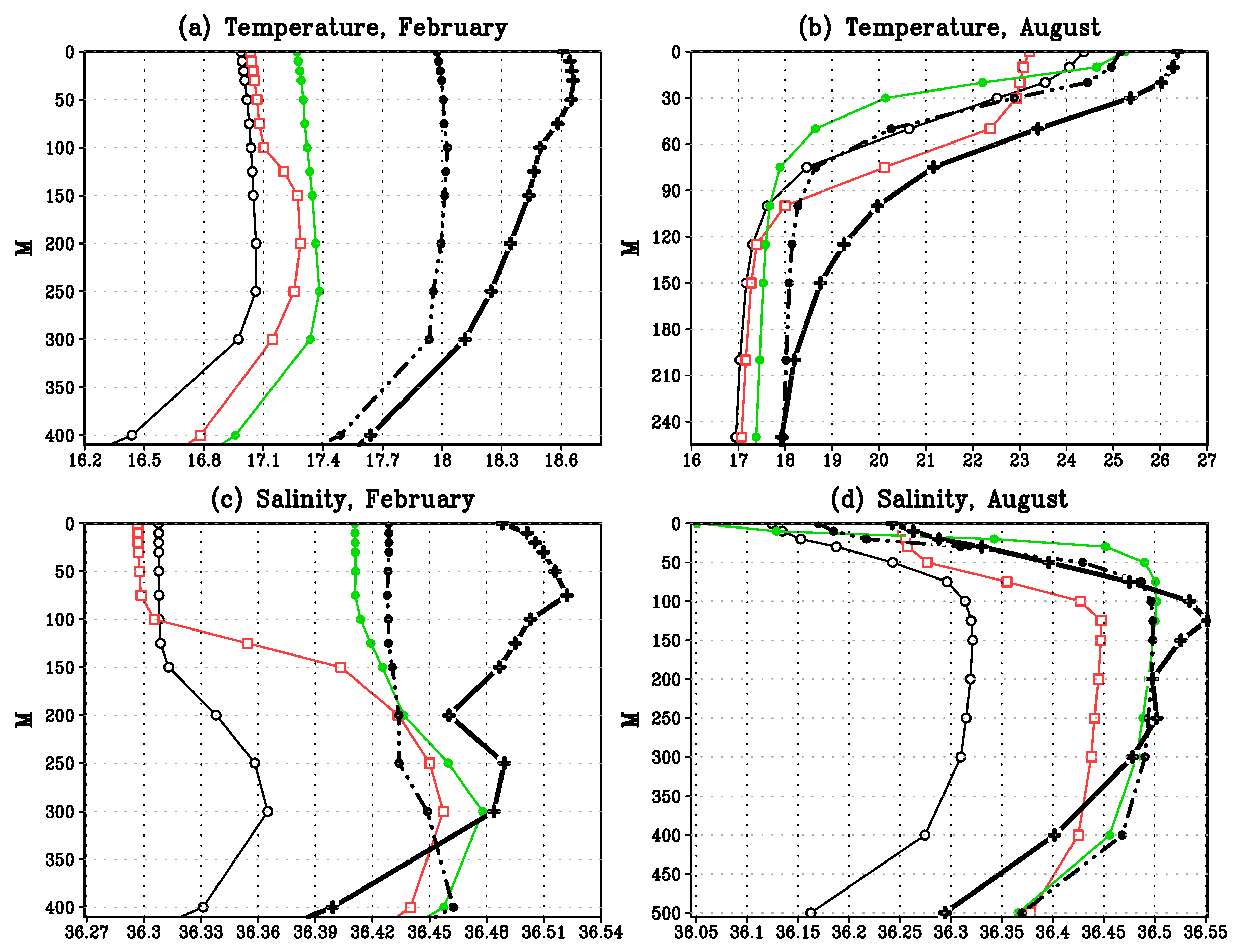
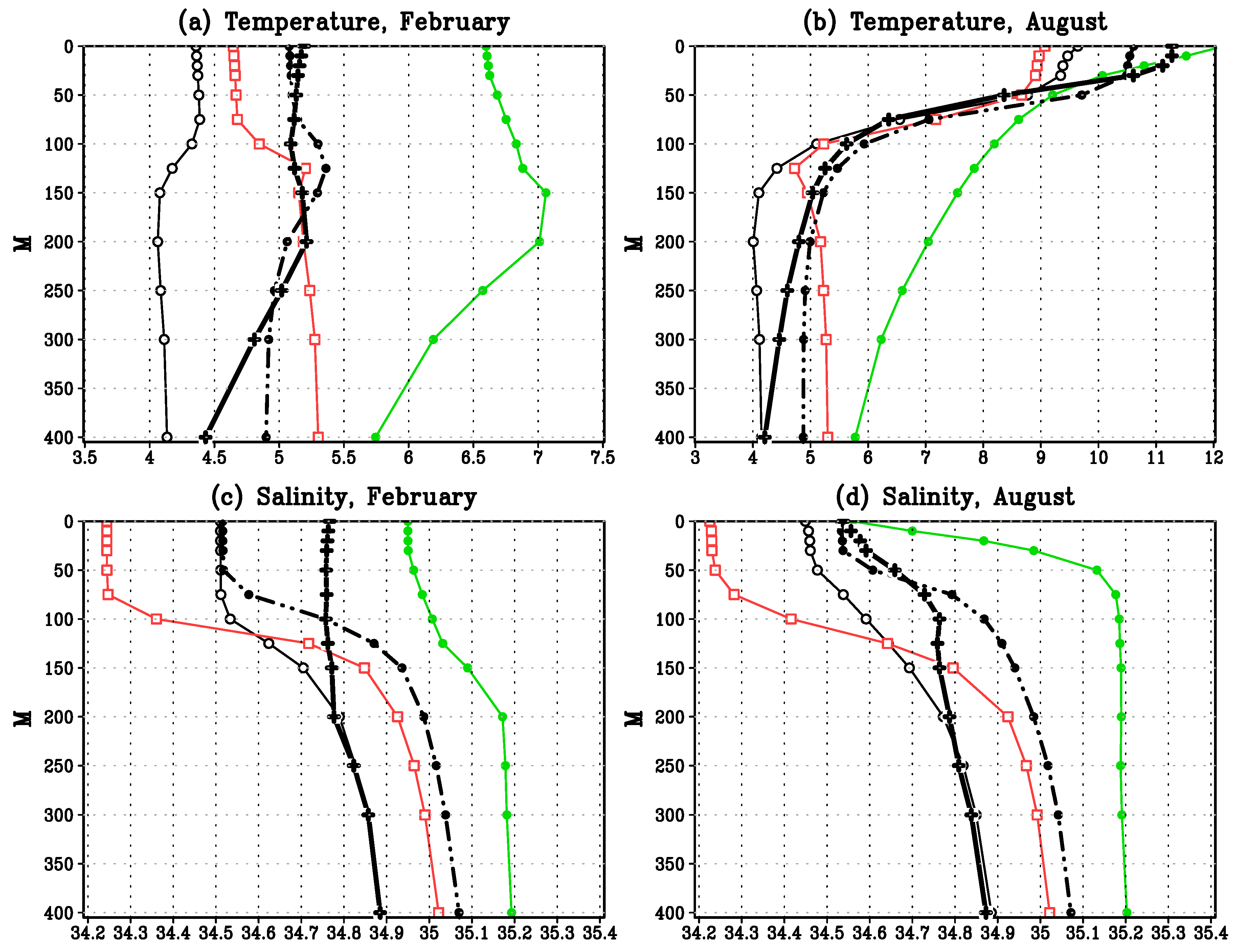
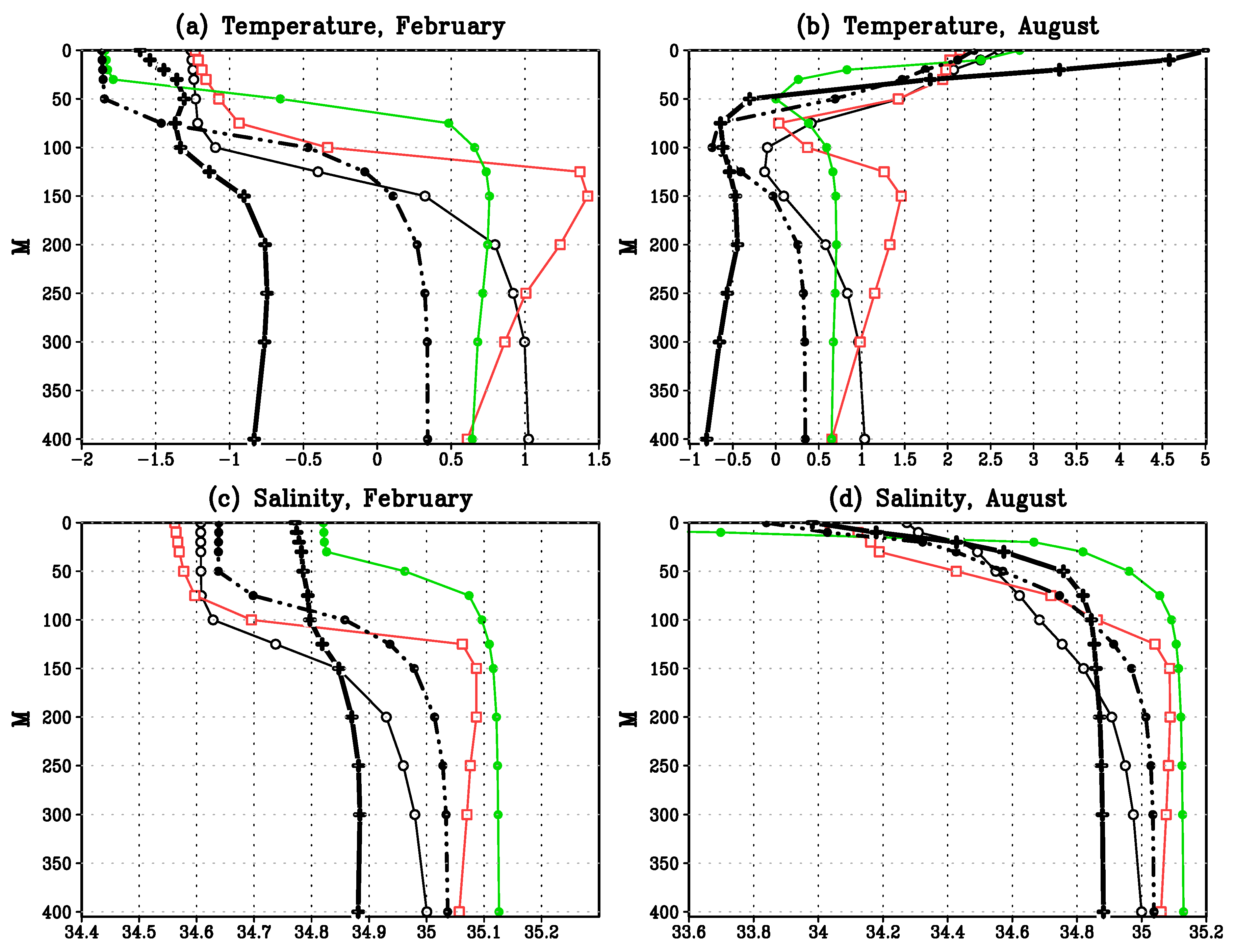
4.1. Comparison to the Generalized Observational Data

We use the data of the World Ocean Atlas for temperature T C l [41] and salinity S C l [42]. Consider the spatial distribution of the model T and S deviation from climatic data T C l and S C l and quality of reproducing vertical structure of the ocean upper layer.
Deviation of simulated temperature and salinity from the climatic data in the ocean upper layer. Denote the differences “model minus climate” for T and S as d T and d S respectively for the period 1963–2009. d T are in the range ± ( 0.2 0.7 )   C in the predominant part of the domain for the EX1, EX2 and EX3 in 0–30 m layer (Figure 1). Temperature in the EX1 is more than a one degree lower than the climatic data in the Equatorial currents, Sargasso and Norwegian seas. Using the AMBF in the EX2 significantly reduces d T in comparison to the EX1 (see Figure 1a,b). Negative d T of more than 2 C disappear in the EX2 on the Equator and in the Tropics. Square of negative deviations more than 1 C are halved. As well, negative d T decrease significantly in the Caribbean sea and African upwelling area. There is a significant decrease in positive d T in the Gulf Stream, the North Atlantic and Labrador currents. Negative d T in the EX3 at the Equator, in the Caribbean and Norwegian Seas, in the African upwelling region decrease even more (see Figure 1c). However, the positive d T in the EX1 and EX2 change to the negative ones in the EX3 for the North Atlantic Current. It is due to the additional entrainment of cold water from the seasonal thermocline by decreasing the Prandtl number relative to the EX1 and EX2.
d S are in the range of ±(0.02–0.1) PSU in the greater part of the domain for all the experiments in the 0–30 m layer (Figure 2). Simulated S > S C l at the Equator, in the Guiana Current and the Gulf Stream, in the Canadian sector of the Arctic. d S reaches 0.5 PSU in the EX3 in the region of the Subpolar Gyre of the North Atlantic (Figure 2c). The same disadvantages are in the EX4. These disadvantages of the EX4 and EX3 are substantially reduced in the EX1 and EX2. Module of d S reduced for EX2 on the Equator, Tropics and Subtropics, North Atlantic, Nordic Seas (Figure 2). T S diagrams are reproduced most realistically for the EX1 and EX2. Deviations d T and d S are compensated in the density in all the experiments in different degree: for d T > 0 , d S > 0 and for d T < 0 , d S < 0 . The best compensation is observed in the EX2.
The greatest positive d S in 0.5–2.0 PSU and d T up to 5–6 C occur in the frontal zone of the Gulf Stream for all experiments (Figure 1 and Figure 2). These high d T and d S can be related both to the relatively coarse spatial resolution of the model and to the complex dynamics in the zone of high T and S gradients. Data on the climatic variables T C l and S C l in this region may experience appreciable variations depending on the change in the amount of observations. The compensation of d T and d S in the density allows to reproduce realistic currents, front dynamics, meanders and eddies.
Vertical structure of the upper ocean layer. We choose the “climatic” period of 30 years 1980–2009 to compare simulated T and S profiles to the ones from the Ocean Atlas. The most observations were performed for this period. We compare the profiles of simulated T and S mean for thirty February and August for 1980–2009 with the climatic monthly mean T C l and S C 1 for February and August [41,42]. February is period of the greatest loss of buoyancy by the ocean. August is month of the greatest inflow of buoyancy from the atmosphere to the ocean. We choose the regions with the most different mixing conditions.
Deviation of T ( z ) for the EX2 from the climatic one decreases by 0.7–0.9 C in the 0–300 m layer relative to the other experiments in the Sargasso Sea in February (Figure 3a). Zone of developed turbulence increases for EX2 in August relative to the EX1, and seasonal thermocline is closer to the observations (Figure 3b). Negative 3 C deviation of T ( z ) from T C l ( z ) exists in the 0–50 m layer for EX4 in August. There is no such deviation for the EX2. Salinity deviations from climate in the EX4 and EX3 are noticeable, especially in the February (Figure 3c). The S profiles are the best reproduced in the EX1 and, especially, in EX2 (Figure 3c,d). EX2 better simulates T and S profiles relative to the other experiments both during August and February in the Sargasso Sea (Figure 3).
Significant deviations of profiles T and S from climatic values for the EX1 are eliminated for the EX2 in the central part of the North Atlantic Current (Figure 4). These deviations were not for the first 20 years of the EX1. Thermocline is very well reproduced in the August for EX2 (Figure 4b). Temperature profiles are better simulated in the EX2 relative to the other experiments in February and August (Figure 4a,b). The main drawback of the parameterization EX4 is high deviation of salinity profiles from the climatic data (Figure 4c,d). The salinity profiles are the best reproduced in the EX2 and EX3 (Figure 4c,d).
Thermal inversion is maintained by the stratification of salinity in the recirculation zone of the West Spitsbergen Current all year round (Figure 5). Vertical structure of T and S for the EX2 is in the maximum agreement with the climatic data relative to the other experiments over here. This is particularly true for the reproduction of a typical cold water interlayer in the 50–130 m layer (see Figure 5b). As well, the EX3 yields a good approximation to the climatic data. EX4 overestimates the salinity gradient in the winter halocline in the layer 50–100 m (Figure 5c) that leads to unreal great temperature inversion (Figure 5a). This drawback overcomes in the experiments using the splitting turbulence algorithm (STA).
In general, the use of STA in mixing parameterization for the OGCM significantly reduces the salinity deviation from climatic data compared to the EX4 (Figure 3c,d, Figure 4c,d and Figure 5c,d). The vertical distributions of T and S in the EX2 (using AMBF) are in the best agreement with climatic data.

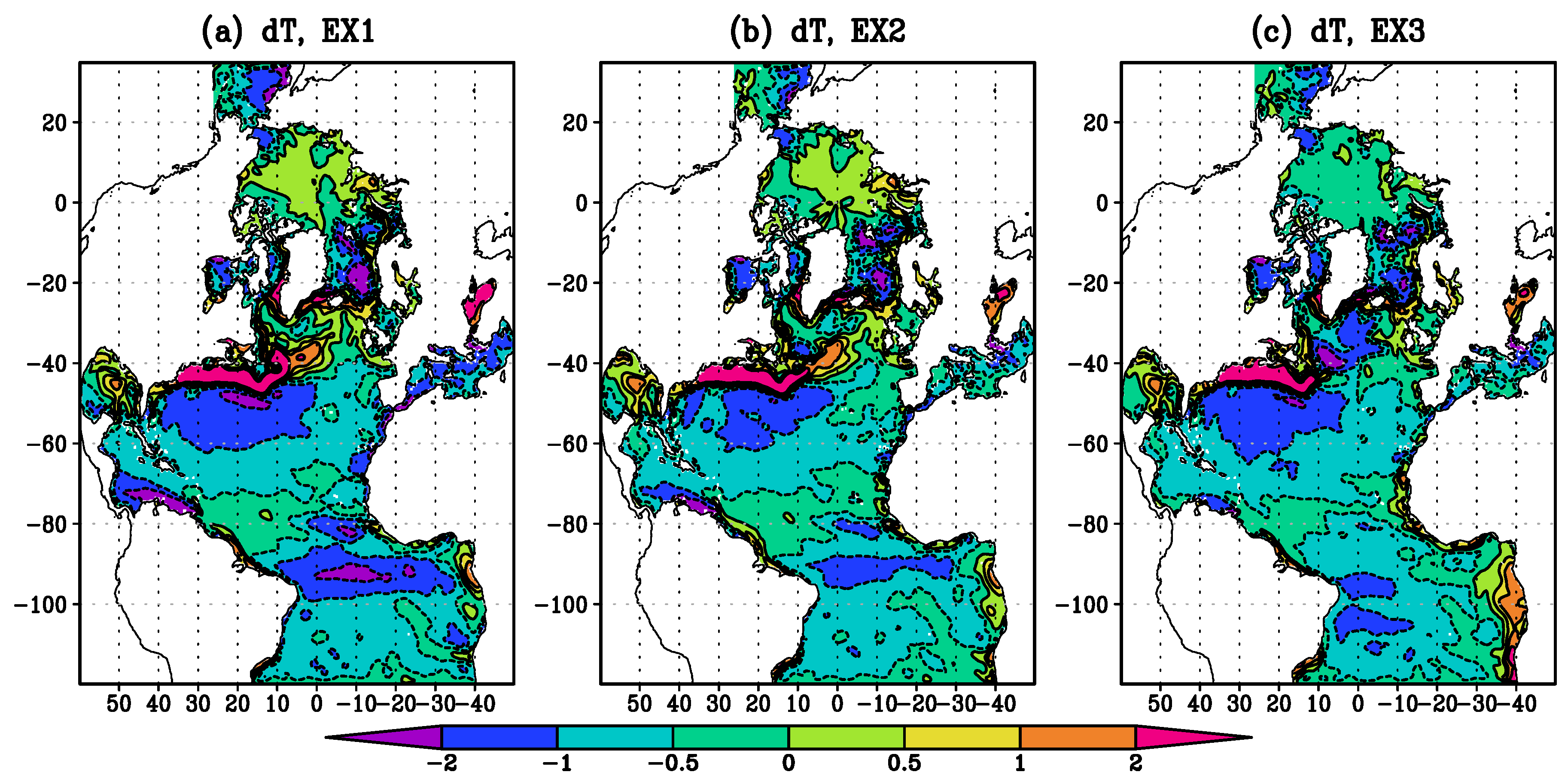
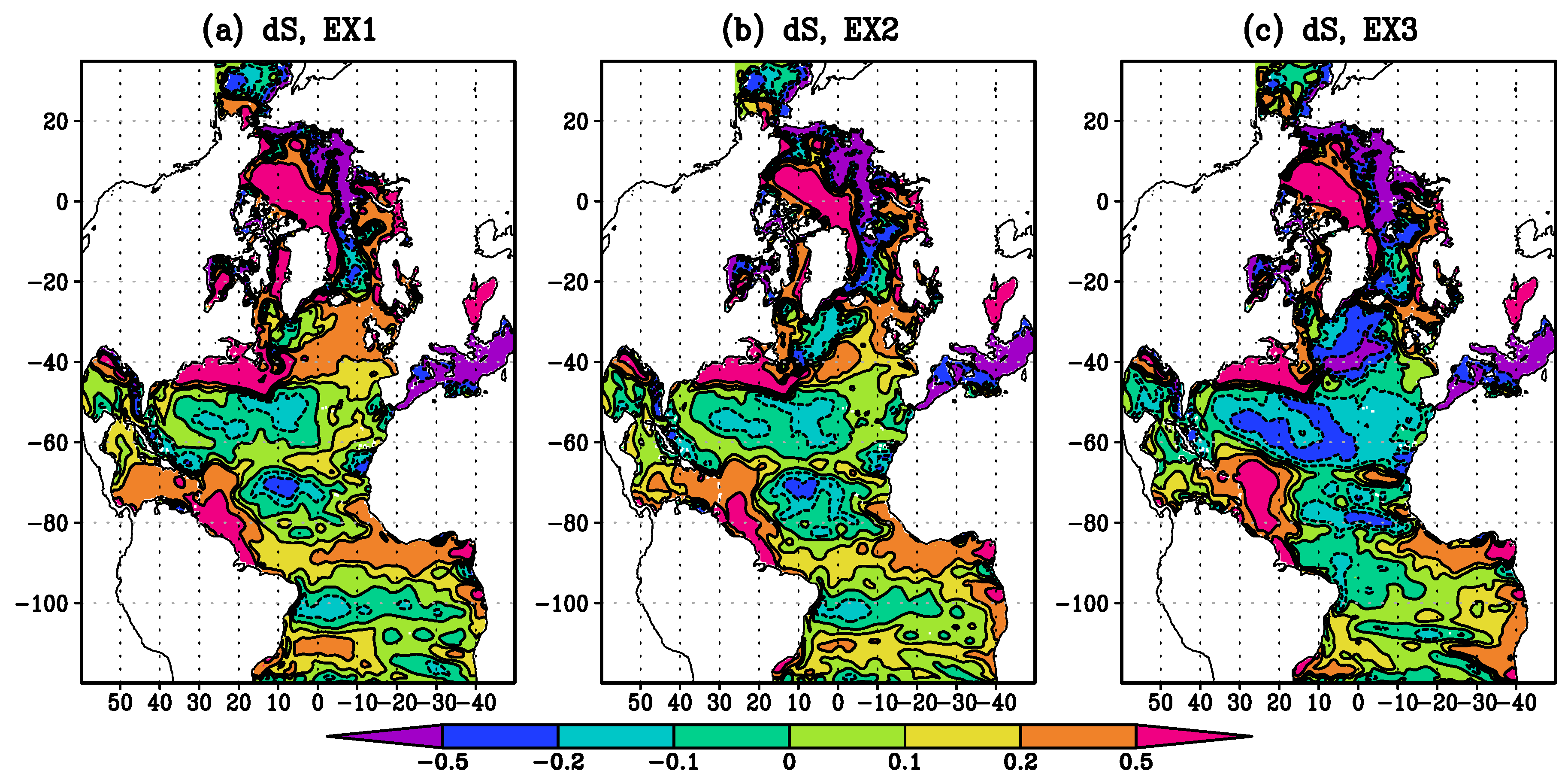
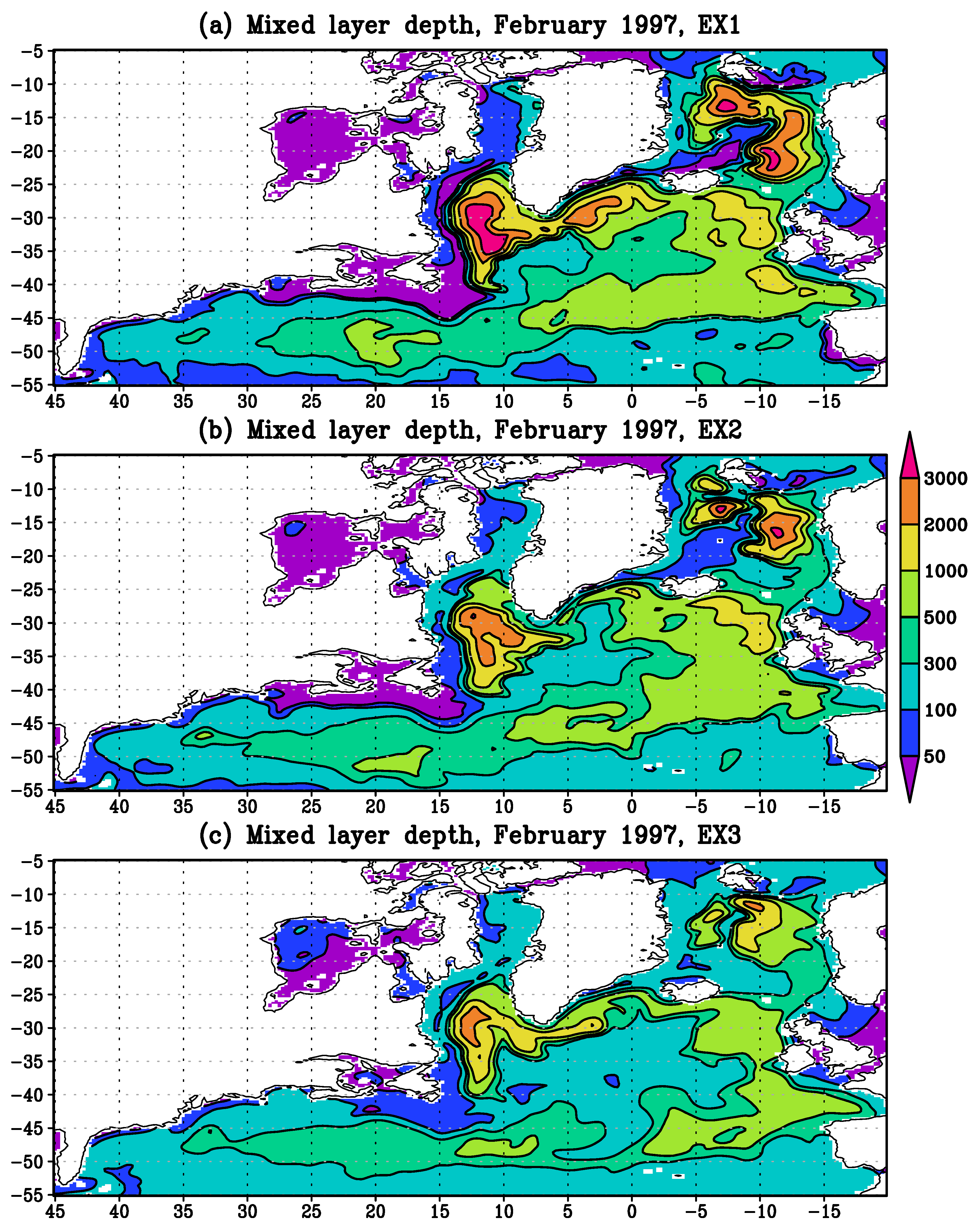
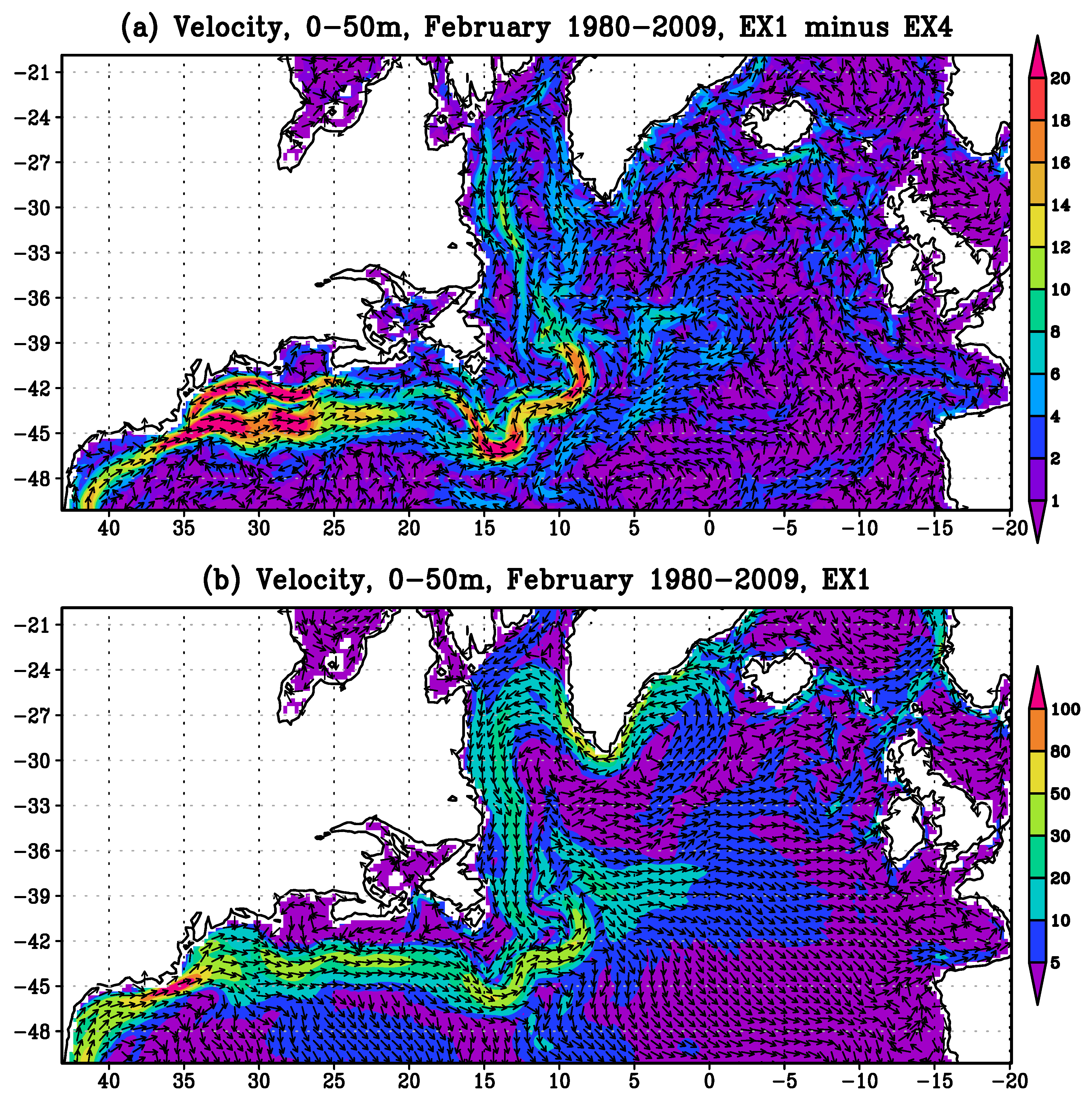
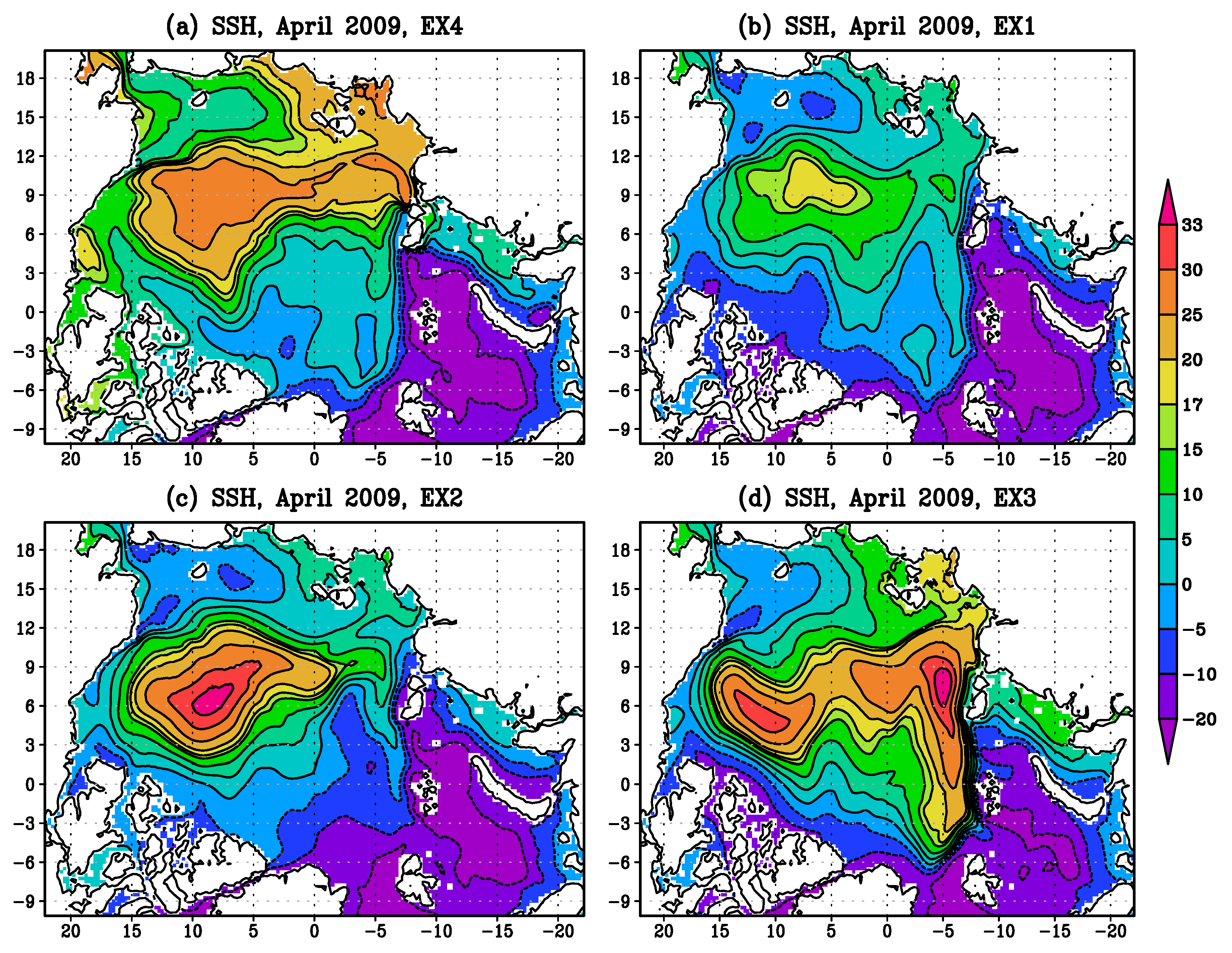
4.2. Sensitivity of Ocean Model Characteristics to the Changes in Mixing Parametrization

The analysis of model sensitivity to the changes in mixing parametrization is accompanied by qualitative comparison of the upper mixed layer (UML) depth, currents and sea surface height (SSH) to the observations.
Thickness of the ocean upper mixed layer. Distribution of the maximum UML depth in the North Atlantic is shown in the Figure 6. This distribution is typical for all winters of the whole period 1948–2009. Maximum UML depth is defined as the level where water density differs from the sea surface density less than 0.15 kg/m 3 . UML depth is highly sensitive to the used parameterizations (Figure 6). UML depth reaches 2–3 km in the Labrador, Norwegian and Greenland seas for the EX1. Area of these regions are sharply reduced for the EX2. UML depth is nowhere greater than 3 km for the EX3. Distribution and values of the UML depth are most similar to their estimates from observations [44] for the EX2 and EX3. EX3 reproduces a deeper UML than the EX1 and EX2 in the frontal zone of the Gulf Stream (Figure 6). The reason for this is in the greater diffusivity of heat and salt due to the smaller Prandtl numbers in the zone of decaying turbulence at relatively small UML depths.
Ocean currents. Changes in the fields of temperature, salinity and density associated with the change in the mixing parameterization cover almost the entire upper half of the baroclinic layer (Figure 3, Figure 4 and Figure 5). This causes a high sensitivity of the circulation and SSH to the change of the mixing parameterization. The greatest changes in ocean currents happen by the transition from parameterization EX4 using a simple dependence of the turbulent coefficients on the Richardson number to EX1–EX3 where STA is used.
Vectors of the velocity difference between EX1–EX3 using STA and EX4 are collinear with the mean circulation vectors in the Gulf Stream and Subpolar Gyre of the North Atlantic for the 0–50 m layer during 1980–2009 (Figure 7). There is an increase in velocities for EX1-EX3 by 20 cm/s and more relative to EX4. Maximum velocity increase occurs in the Gulf Stream separation from the coast (Figure 7a). This brought the current velocities closer to real values. Differences in the velocity between the EX1, EX2 and EX3 can reach 5–10 cm/s in the 0–50 m layer in separate regions. The results show that using AMBF in the EX2 allows to reproduce thermohaline characteristics better, and it should be recommended to use AMBF for computation of circulation.
Sea surface height. SSH is also sensitive to the change of parameterizations. SSH is associated with the annual cycle of sea ice extent. Figure 8 shows the SSH simulated in the EX4 (a), EX1 (b), EX2 (c) and EX3 (d), for the 62nd year of integration in April 2009. Sea ice extent reached its maximum in this month for the Arctic Ocean and Nordic Seas (NSIDC data). Beaufort Gyre is here the most characteristic feature of the circulation and SSH field. SSH distribution is more similar to the reconstruction according to the climatic data [38] for the EX2 relative to the other experiments. Beaufort Gyre is better expressed in the SSH field for EX2. Unrealistic overestimation of SSH was obtained for the EX4 in the region of the Siberian shelf. The greatest difference in the maximum SSH between the EX2 and EX1 is 15 cm in the Beaufort Gyre. EX3 reproduces high SSH values on the periphery of the Beaufort Gyre due to the steric effect as the result of the greater entrainment of dense water from the pycnocline into the upper ocean layer (Figure 8d). So, SSH is reproduced most realistically in the EX2 with taking into account the AMBF in the equations of turbulence (Figure 8c).
Heat flux at the ocean surface. Heat fluxes at the upper boundary of the ocean are calculated using the model SST. Model SST depends on turbulent mixing in its upper layer. Thus, the forcing for the OGCM also depends on the used mixing parameterization. Typical example for the sum of the latent L E and sensible Q T heat fluxes shows that the space distributions of the heat fluxes are close to each other in the EX1, EX2 and EX3 for the period of maximum heat loss by the ocean in February (Figure 9). However, quantitative differences of fluxes can reach 50–200 W/m 2 in some regions. For example, sensitivity of the heat fluxes to the change of the mixing parameterization revealed in the subtropics. Low heat losses L E + Q T < 50 W/m 2 for EX1 changes to greater ones for the EX2 (Figure 9a,b). This is due to the following process. Turbulence zone penetrates to deeper layers in the preceding warm period for the EX2. Greater accumulation of heat in the upper ocean layer occurs. More significant water-air temperature differences for the EX2 relative to the EX1 arises in the winter.

4.3. Turbulent Energy and Omega

The spatial distribution and temporal evolution of TKE and TDF, differing from one experiment to another, are generally similar in EX1, EX2 and EX3. In all the experiments, the period of turbulence temporal variability ( 1 / ω ) varies from seconds in layers of high density gradients, to several minutes in well-mixed layers. Such quantities are close to the observations [45]. In the evolution of TKE and TDF, the annual cycle is well pronounced. Against this background, there is a very high synoptic variability of these characteristics over time. Figure 10 shows the TKE field for the 62nd year of integration (2009) in the 0–30 m layer (for August). Zones of the Northern Trade winds and Westerlies in the Northern Hemisphere are marked with high TKE values ∼50–100 cm 2 /s 2 associated with high wind speeds. Low TKE values of 1–3 cm 2 /s 2 are observed in Horse Latitudes and the Intertropical Convergence zone. South of the Equator, the TKE values of 100–150 cm 2 /s 2 are due to the loss of heat by the ocean in the winter of the Southern Hemisphere.

4.4. Numerical Aspects, Data Assimilation

One of the rapidly developing areas of numerical modelling of the oceanic and marine circulation is the assimilation of observational data [46,47,48,49,50,51]. In the nearest future, we plan to develop a high-resolution model of the Arctic Ocean and include in it 4D VAR data assimilation procedure. A successful solution of this problem is connected with the choice of an economical numerical algorithm for solving the optimality system—a coupled system of forward and adjoint ocean dynamics equations [50]. Here we can use the developed algorithm to solve the k ω turbulence equations. The algorithm is based on an effective splitting technique with respect to physical processes. The formulation of an individual splitting stage describing the generation-dissipation process, allows one to solve them analytically which determines the computational efficiency. Our experiments showed the computational efficiency of the algorithm for forward simulation of Arctic—North Atlantic general circulation. This algorithm, in our opinion, will also be effective in solving 4D VAR data assimilation problems.

5. Summary

New results in the problem of vertical mixing parameterization for the ocean general circulation model (OGCM) are shown at the example of the simulation of climatic characteristics for North Atlantic and Arctic Ocean for 1948–2009. Like OGCM equations, turbulence equations are solved using multicomponent splitting methods. This allowed us to rationally improve the mixing parametrization using the k ω model. A new splitting algorithm is proposed for solving turbulence equations that allows to reduce the complete system to the stages of transport-diffusion and generation-dissipation. An analytical solution was found for the k ω equations at the generation-dissipation splitting stage that is impossible for k k l and k ϵ closures. This opens new possibilities to control ocean characteristics of the OGCM’s numerical experiments by means of some physical factors through coefficients of the proposed analytical k ω model solution. We demonstrate examples of possibilities for controlling the OGCM solution by such physical factors as climatic annual mean buoyancy frequency (AMBF) and Prandtl number as function of the Richardson number.
For this purpose, the OGCM INMOM coupled with a two equation k ω turbulence model is used for simulation of hydrophysical fields in the North Atlantic and Arctic Ocean. The model has horizontal resolution 0.25 with 40 σ -levels along the depth.
The numerical results show the model’s satisfactory performance in simulating large-scale ocean circulation and upper layer dynamics. The deviations between simulated and observed temperature and salinity in the upper mixed layer are about ±(0.2–0.7) C and ±(0.02–0.10) PSU respectively. The vertical structure of temperature and salinity and their gradients in the pycnocline are acceptably reproduced. The simulations show that taking into account of the AMBF data improves the reproduction of temperature and salinity in the upper ocean layer. During the warm-up period in the tropics, accounting AMBF data increases zones of developed turbulence and makes the seasonal thermocline more realistic. In the Subarctic, Greenland and Norwegian seas, the temperature inversion and cold intermediate layer are more realistically reproduced. The experiments demonstrate that taking into account AMBF improves reproduction of the large-scale thermohaline and dynamical characteristics. Prandtl number variations improve the upper mixed layer depth simulation especially for high latitudes.
Replacement of the simple relation between turbulent viscosity and diffusion and the Richardson number [8] by k ω parameterization increases velocity of currents in the upper 50 m layer by 10–20 cm/s or more. This is noticeable for the Gulf Stream, Greenland, Labrador and North Atlantic currents. The Subpolar Gyre of the North Atlantic becomes more intense and realistic. The SSH is also sensitive to the choice of turbulent parameterization. The largest SSH difference in the center of the Beaufort Gyre between different runs is about 15 cm. In experiments with the analytical solution of the k ω equations, SSH in the Beaufort Gyre is well reproduced, especially with taking into account the AMBF in the equations of turbulence. Experiments with the Prandtl number tuning show that the increase of pycnocline waters entrainment into the mixed layer due to the steric effect has a significant influence on the Arctic Ocean circulation.
The experiments also demonstrate the computational effectiveness of the proposed approach based on the splitting method with respect to physical processes. We split k ω equations into the two main stages describing transport-diffusion and generation-dissipation processes. At the generation-dissipation stage, the equation for ω does not depend on k. It allows us to solve both turbulence equations analytically that ensures high computational efficiency.

Author Contributions

Methodology, V.Z.; Software Development, S.M., A.G.; Validation, S.M., A.G.; Formal Analysis, S.M.; Investigation, S.M.; Data Curation, A.G.; Performing Simulations, A.G.; Writing Original Draft Preparation, S.M., V.Z. and A.G.; Visualization, A.G.; Supervision, V.Z.

Funding

This research was funded by the Russian Science Foundation (grant No. 17-77-30001). The simulations with INMOM were performed under support of the Russian Foundation for Basic Research (grants No. 16-05-00534 and 18-05-00177).

Conflicts of Interest

The authors declare no conflict of interest. The founding sponsors had no role in the design of the study; in the collection, analyses, or interpretation of data; in the writing of the manuscript, and in the decision to publish the results.

Abbreviations

The following abbreviations are used in this manuscript:
AMBFAnnual Mean Buoyancy Frequency
INMOMInstitute of Numerical Mathematics Ocean Model
OGCMOcean General Circulation Model
STASplitting Turbulence Algorithm

References

  1. Ibrayev, R.; Khabeev, R.; Ushakov, K.V. Eddy-resolving 1/10° model of the World Ocean. Izv. Atmos. Ocean. Phys. 2012, 48, 37–46. [Google Scholar] [CrossRef]
  2. Maslowski, W.; Kinney, J.; Marble, D.; Jakacki, J. Towards Eddy-Resolving Models of the Arctic Ocean. In Ocean Modeling in an Eddying Regime; American Geophysical Union: Washington, DC, USA, 2013; pp. 241–264. [Google Scholar] [CrossRef]
  3. Mellor, G. Users guide for a three-dimensional, primitive equation, numerical ocean model. In Program in Atmospheric and Oceanic Sciences; Princeton University: Princeton, NJ, USA, 2004. [Google Scholar]
  4. Zalesny, V.; Gusev, A. Mathematical model of the World Ocean dynamics with algorithms of variational assimilation of temperature and salinity fields. Russ. J. Numer. Anal. Math. Model. 2009, 24, 171–191. [Google Scholar] [CrossRef]
  5. Zalesny, V.; Marchuk, G.; Agoshkov, V.; Bagno, A.; Gusev, A.; Diansky, N.; Moshonkin, S.; Tamsalu, R.; Volodin, E. Numerical simulation of large-scale ocean circulation based on the multicomponent splitting method. Russ. J. Numer. Anal. Math. Model. 2010, 25, 581–609. [Google Scholar] [CrossRef]
  6. Sarkisyan, A.; Sündermann, J. Modelling Ocean Climate Variability; Springer Science+Business Media B.V.: Berlin, Germany, 2009; p. 374. [Google Scholar]
  7. Moshonkin, S.; Alekseev, G.; Bagno, A.; Gusev, A.; Diansky, N.; Zalesny, V. Numerical simulation of the North Atlantic—Arctic Ocean—Bering Sea circulation in the 20th century. Russ. J. Numer. Anal. Math. Model. 2011, 26, 161–178. [Google Scholar] [CrossRef]
  8. Pacanowski, R.; Philander, S. Parameterization of Vertical Mixing in Numerical Models of Tropical Oceans. J. Phys. Oceanogr. 1981, 11, 1443–1451. [Google Scholar] [CrossRef] [Green Version]
  9. Moshonkin, S.; Gusev, A.; Zalesny, V.; Byshev, V. Mixing parameterizations in ocean climate modeling. Izv. Atmos. Ocean. Phys. 2016, 52, 196–206. [Google Scholar] [CrossRef]
  10. Moshonkin, S.; Tamsalu, R.; Zalesny, V. Modeling sea dynamics and turbulent zones on high spatial resolution nested grids. Oceanology 2007, 47, 747–757. [Google Scholar] [CrossRef]
  11. Moshonkin, S.; Zalesny, V.; Gusev, A.; Tamsalu, R. Turbulence modeling in ocean circulation problems. Izv. Atmos. Ocean. Phys. 2014, 50, 49–60. [Google Scholar] [CrossRef]
  12. Noh, Y.; Kang, Y.; Matsuura, T.; Iizuka, S. Effect of the Prandtl number in the parameterization of vertical mixing in an OGCM of the tropical Pacific. Geophys. Res. Lett. 2005, 32, L23609. [Google Scholar] [CrossRef]
  13. Noh, Y.; Ok, H.; Lee, E.; Toyoda, T.; Hirose, N. Parameterization of Langmuir Circulation in the Ocean Mixed Layer Model Using LES and Its Application to the OGCM. J. Phys. Oceanogr. 2016, 46, 57–78. [Google Scholar] [CrossRef]
  14. Semenov, E. Numerical modeling of White Sea dynamics and monitoring problem. Izv. Atmos. Ocean. Phys. 2004, 40, 114–126. [Google Scholar]
  15. Warner, J.; Sherwood, C.; Arango, H.; Signell, R. Performance of four turbulence closure models implemented using a generic length scale method. Ocean Modell. 2005, 8, 81–113. [Google Scholar] [CrossRef]
  16. Kantha, L.; Clayson, C. An improved mixed layer model for geophysical applications. J. Geophys. Res. Oceans 1994, 99, 25235–25266. [Google Scholar] [CrossRef]
  17. Kolmogorov, A. Equations of turbulent motion of an incompressible fluid. Izv. Acad. Sci. USSR Phys. Ser. 1942, 6, 56–58. [Google Scholar]
  18. Mellor, G.; Yamada, T. A Hierarchy of Turbulence Closure Models for Planetary Boundary Layers. J. Atmos. Sci. 1974, 31, 1791–1806. [Google Scholar] [CrossRef] [Green Version]
  19. Saffman, P. A model for inhomogeneous turbulent flow. Proc. R. Soc. Lon. A Math. Phys. Eng. Sci. 1970, 317, 417–433. [Google Scholar] [CrossRef]
  20. Umlauf, L.; Burchard, H. A generic length-scale equation for geophysical turbulence models. J. Mar. Res. 2003, 61, 235–265. [Google Scholar] [CrossRef]
  21. Mellor, G.; Yamada, T. Development of a turbulence closure model for geophysical fluid problems. Rev. Geophys. 1982, 20, 851–875. [Google Scholar] [CrossRef]
  22. Noh, Y.; Min, H.; Raasch, S. Large Eddy Simulation of the Ocean Mixed Layer: The Effects of Wave Breaking and Langmuir Circulation. J. Phys. Oceanogr. 2004, 34, 720–735. [Google Scholar] [CrossRef]
  23. Madec, G.; The NEMO Team. NEMO Ocean Engine. TKE Turbulent Closure Scheme; Note du Pôle de modélisation, Institut Pierre-Simon Laplace (IPSL): France, 2016. [Google Scholar]
  24. Umlauf, L.; Burchard, H.; Hutter, K. Extending the kω turbulence model towards oceanic applications. Ocean Modell. 2003, 5, 195–218. [Google Scholar] [CrossRef]
  25. Canuto, V.; Howard, A.; Cheng, Y.; Muller, C.; Leboissetier, A.; Jayne, S. Ocean turbulence, III: New GISS vertical mixing scheme. Ocean Modell. 2010, 34, 70–91. [Google Scholar] [CrossRef] [Green Version]
  26. Marchuk, G. Methods of Numerical Mathematics, 2nd ed.; Stochastic Modelling and Applied Probability; Springer: New York, NY, USA, 2009. [Google Scholar]
  27. Zalesny, V.; Gusev, A.; Ivchenko, V.; Tamsalu, R.; Aps, R. Numerical model of the Baltic Sea circulation. Russ. J. Numer. Anal. Math. Model. 2013, 28, 85–100. [Google Scholar] [CrossRef]
  28. Brydon, D.; Sun, S.; Bleck, R. A new approximation of the equation of state for seawater, suitable for numerical ocean models. J. Geophys. Res. Oceans 1999, 104, 1537–1540. [Google Scholar] [CrossRef] [Green Version]
  29. Yakovlev, N. Reproduction of the large-scale state of water and sea ice in the Arctic Ocean in 1948–2002: Part I. Numerical model. Izv. Atmos. Ocean. Phys. 2009, 45, 357–371. [Google Scholar] [CrossRef]
  30. Burchard, H.; Bolding, K.; Villarreal, M. GOTM, A General Ocean Turbulence Model: Theory, Implementation and Test Cases; EUR/European Commission, Space Applications Institute: Gujarat, India, 1999. [Google Scholar]
  31. Miropolski, Y.Z. Non-stationary model of the layer of the convective-wind mixing in the ocean. Izv. Atmos. Ocean. Phys. 1970, 6, 1284–1294. [Google Scholar]
  32. Zaslavskii, M.; Zalesny, V.; Kabatchenko, I.; Tamsalu, R. On the self-adjusted description of the atmospheric boundary layer, wind waves, and sea currents. Oceanology 2006, 46, 159–169. [Google Scholar] [CrossRef]
  33. Marchuk, G. Splitting and alternative direction methods. In Handbook of Numerical Analysis; Ciarlet, P., Lions, J., Eds.; Springer: Amsterdam, The Netherlands, 1990; pp. 197–462. [Google Scholar]
  34. Lebedev, V. Difference analogies of orthogonal decompositions of basic differential operators and some boundary value problems. J. Comput. Math. Math. Phys. 1964, 4, 449–465. [Google Scholar]
  35. Mesinger, F.; Arakawa, A. (Eds.) Global Atmospheric Research Program World Meteorological Organization: Switzerland. In Numerical Methods Used in Atmospheric Models; Wiley: Hoboken, NJ, USA, 1976; Volume 1. [Google Scholar]
  36. National Geophysical Data Center, NOAA. 2-Minute Gridded Global Relief Data (ETOPO2) V2; National Geophysical Data Center: Boulder, MT, USA, 2006. [CrossRef]
  37. Large, W.; Yeager, S. The global climatology of an interannually varying air–sea flux data set. Clim. Dyn. 2009, 33, 341–364. [Google Scholar] [CrossRef]
  38. Steele, M.; Morley, R.; Ermold, W. PHC: A Global Ocean Hydrography with a High-Quality Arctic Ocean. J. Clim. 2001, 14, 2079–2087. [Google Scholar] [CrossRef]
  39. Blanke, B.; Delecluse, P. Variability of the Tropical Atlantic Ocean Simulated by a General Circulation Model with Two Different Mixed-Layer Physics. J. Phys. Oceanogr. 1993, 23, 1363–1388. [Google Scholar] [CrossRef] [Green Version]
  40. Unesco. Tenth Report of the Joint Panel on Oceanographic Tables and Standards: Sidney, B.C., Canada 1–5 SEptember 1980 Sponsored by Unesco, ICES, SCOR, IAPSO; Unesco Technical Papers in Marine Science; UNESCO: Paris, France, 1981. [Google Scholar]
  41. Locarnini, R.; Mishonov, A.; Antonov, J.; Boyer, T.; Garcia, H.; Baranova, O.; Zweng, M.; Johnson, D. World Ocean Atlas 2009, Volume 1: Temperature; Levitus, S., Ed.; NOAA Atlas NESDIS 68; U.S. Government Printing Office: Washington, DC, USA, 2010; p. 184.
  42. Antonov, J.; Seidov, D.; Boyer, T.; Locarnini, R.; Mishonov, A.; Garcia, H.; Baranova, O.; Zweng, M.; Johnson, D. World Ocean Atlas 2009, Volume 2: Salinity; Levitus, S., Ed.; NOAA Atlas NESDIS 69; U.S. Government Printing Office: Washington, DC, USA, 2010; p. 184.
  43. Munk, W.; Anderson, E. Notes on a theory of the thermocline. J. Mar. Res. 1948, 7, 276–295. [Google Scholar]
  44. De Boyer Montégut, C.; Madec, G.; Fischer, A.; Lazar, A.; Iudicone, D. Mixed layer depth over the global ocean: An examination of profile data and a profile-based climatology. J. Geophys. Res. Oceans 2004, 109, C12003. [Google Scholar] [CrossRef]
  45. Monin, A.; Ozmidov, R. Oceanic Turbulence; Hydrometeoizdat: Leningrad, Russia, 1981; p. 320. [Google Scholar]
  46. Blum, J.; Le Dimet, F.; Navon, I. Data Assimilation for Geophysical Fluids. In Special Volume: Computational Methods for the Atmosphere and the Oceans; Temam, R., Tribbia, J., Eds.; Handbook of Numerical Analysis; Elsevier: New York, NY, USA, 2009; Volume 14, pp. 385–441. [Google Scholar]
  47. Marchuk, G.; Paton, B.; Korotaev, G.; Zalesny, V. Data-computing technologies: A new stage in the development of operational oceanography. Izv. Atmos. Ocean. Phys. 2013, 49, 579–591. [Google Scholar] [CrossRef]
  48. Korotaev, G.; Oguz, T.; Dorofeyev, V.; Demyshev, S.; Kubryakov, A.; Ratner, Y. Development of Black Sea nowcasting and forecasting system. Ocean Sci. 2011, 7, 629–649. [Google Scholar] [CrossRef] [Green Version]
  49. Korotaev, G.; Saenko, O.; Koblinsky, C. Satellite altimetry observations of the Black Sea level. J. Geophys. Res. Oceans 2001, 106, 917–933. [Google Scholar] [CrossRef] [Green Version]
  50. Agoshkov, V.; Zalesny, V. Variational Data Assimilation Technique in Mathematical Modeling of Ocean Dynamics. Pure Appl. Geophys. 2012, 169, 555–578. [Google Scholar] [CrossRef]
  51. Zalesny, V.; Agoshkov, V.; Shutyaev, V.; Le Dimet, F.; Ivchenko, V. Numerical modeling of ocean hydrodynamics with variational assimilation of observational data. Izv. Atmos. Ocean. Phys. 2016, 52, 431–442. [Google Scholar] [CrossRef]
Figure 1. Average for 1963–2009 temperature deviations (in C) in the 0–30 m layer from climatic data [41] in the experiments EX1 (a), EX2 ( α C l = 0.9 ) (b) and EX3 (c). Coordinates of the model: the geographical grid is replaced by a two-pole orthogonal (poles on the geographical equator at points with coordinates 120 W and 60 E). The outlines of continents and islands are shown.
Jmse 06 00095 g001
Figure 2. Average for 1963–2009 deviation of salinity (in PSU) in the 0–30 m layer from the climatic observational data [42] in the experiments EX1 (a), EX2 (b) and EX3 (c). The model coordinates are used (see the caption under Figure 1).
Jmse 06 00095 g002
Figure 3. T (in C) and S (in PSU) profiles for February and August averaged for 1980–2009 in the Sargasso Sea (center of the one-degree model cell near 36 N, 51 W): the columns are February (left) and August (right), rows are temperature (top) and salinity (bottom). Black solid thick line with crosses represents the climate; Green solid line with dark circles—EX1; Black dash/double dot line with dark circles—EX2; Black solid thin line with hollow circles—EX3; Red solid line with hollow squares—EX4.
Jmse 06 00095 g003
Figure 4. T (in C) and S (in PSU) profiles for February and August averaged for 1980–2009 in the North Atlantic Current (center of the one-degree model cell near 52 N, 38 W): the columns are February (left) and August (right), rows are temperature (top) and salinity (bottom). Black solid thick line with crosses represents the climate; Green solid line with dark circles—EX1; Black dash/double dot line with dark circles—EX2; Black solid thin line with hollow circles—EX3; Red solid line with hollow squares—EX4.
Jmse 06 00095 g004
Figure 5. T (in C) and S (in PSU) profiles for February and August averaged for 1980–2009 in the recirculation region of the West Spitsbergen Current (center of the one-degree model cell near 75 N, 2 W): the columns are February (left) and August (right), rows are temperature (top) and salinity (bottom). Black solid thick line with crosses represents the climate; Green solid line with dark circles—EX1; Black dash/double dot line with dark circles—EX2; Black solid thin line with hollow circles—EX3; Red solid line with hollow squares—EX4.
Jmse 06 00095 g005
Figure 6. Maximum thickness of the upper mixed layer (in meters) for the 50th year of integration (February 1997) in the EX1 (a), EX2 (b), EX3 (c) in model coordinates.
Jmse 06 00095 g006
Figure 7. The average in the 0–50 m layer for thirty February of 1980–2009: the difference in the velocities between the EX1 and EX4 (EX1 minus EX4) (a); the velocity in the EX1 (b). The model coordinates are used (see the caption under Figure 1). The direction is shown by vectors, and the magnitude in cm/s is shown by shading.
Jmse 06 00095 g007
Figure 8. Sea surface height (in cm plus 30) in the EX4 (a), EX1 (b), EX2 (c) and EX3 (d) in April 2009 (The 62nd year of integration). April 2009 is the month of the maximum sea ice extent for the Arctic Ocean and Nordic Seas according NSIDC data. The model coordinates are used (see the caption under Figure 1, the point with coordinates (0,0) corresponds to the North Pole).
Jmse 06 00095 g008
Figure 9. The sum of latent and sensible heat fluxes (W/m 2 ) at the ocean surface in February for the 50th year of the runs (1997) in the experiments EX1 (a), EX2 (b) and EX3 (c).
Jmse 06 00095 g009
Figure 10. Turbulent kinetic energy (cm 2 /s 2 ) in the 0–30 m layer in August 2009 (the 62nd year of integration). The model coordinates are used (see the caption under Figure 1).
Jmse 06 00095 g010
Table 1. Model parameters corresponding to the numerical experiments EX1–EX4.
ExperimentsPrandtl NumberComputation of k and ω Accounting AMBFViscosity and Diffusivity
EX1 Pr = 1 , R i 0.2 5 R i , 0.2 < R i < 2 10 , R i 2 , R i = N 2 G 2 A = G 2 N 2 , B = c 1 ω G 2 c 3 ω N 2 α M = 1 , α C l = 0 K U = k ω , K T = K S = K U Pr
EX2 Pr = 1 , R i 0.2 5 R i , 0.2 < R i < 2 10 , R i 2 A = G 2 N s 2 , B = c 1 ω G 2 c 3 ω N s 2 , N s 2 = α M N M 2 + α C l N C l 2 α M = 0.1 , α C l = 0.9 K U = k ω , K T = K S = K U Pr
EX3 Pr = Pr 0 , R i 0.2 a P R i 2 + b P R i + + c P , 0.2 < R i < 2 10 , R i 2 a P = 1.3227 , b P = 2.2487 , c P = 0.2116 , Pr 0 = 0.7143 A = G 2 1 Pr N 2 , B = c 1 ω G 2 c 3 ω Pr N 2 α M = 1 , α C l = 0 K U = k ω , K T = K S = K U Pr
EX4NoNoNo K U = K 0 ( 1 + 5 R i ) 2 + K b , K T = K S = = K U 1 + 5 R i + K T b , K 0 = 100 c m 2 / s , K b = 1 c m 2 / s , K T b = 0.05 c m 2 / s

