A 2D Tide-Averaged Model for the Long-Term Evolution of an Idealized Tidal Basin-Inlet-Delta System


1
Department of Oceanography and Coastal Sciences, Louisiana State University, Baton Rouge, LA 70803, USA
2
Center for Computation and Technology, Louisiana State University, Baton Rouge, LA 70803, USA
*
Author to whom correspondence should be addressed.
J. Mar. Sci. Eng. 2018, 6(4), 154; https://doi.org/10.3390/jmse6040154
Submission received: 17 November 2018
/
Revised: 29 November 2018
/
Accepted: 7 December 2018
/
Published: 11 December 2018
(This article belongs to the Special Issue Large-scale Coastal Behavior)
Abstract
:We present a model for the morphodynamics of tidal basin-inlet-delta systems at the centennial time scales. Tidal flow is calculated through a friction dominated model, with a semi-empirical correction to account for the advection of momentum. Transport of non-cohesive sediment (sand) is simulated through tidal dispersion, i.e., without explicitly resolving sediment advection. Sediment is also transported downslope through a bed elevation diffusion process. The model is compared to a high-resolution tide-resolving model (Delft3D) with good agreement for different hydrodynamic and sedimentary settings. The model has low sensitivity with respect to temporal and spatial discretization. For the same spatial resolution, the model is about five orders of magnitude faster than tide-resolving models (e.g., Delft3D), and about three orders of magnitude faster than tide-resolving models that use a morphological acceleration factor. This numerical efficiency makes the model suitable to assess long-term changes of large coastal areas. The model’s simplicity makes it suitable for coupling with other physical, ecological, and socio-economic dynamics.
1. Introduction
Understanding and predicting how coastal systems will change at long time scales (100–1000 years) would be useful for at least two reasons: to inform long-term adaptation strategies to climate change, and to allow for better comparison with the sedimentary record. Despite this need, long-term predictions remains a great challenge for coastal morphodynamics [1,2].
Even though coastal systems are likely influenced by many interacting processes such as tides, river, and waves, most modeling studies have focused on the idealized case where only tides are present [1,3,4,5,6,7,8,9]. These studies have highlighted how tidal basin-inlet-delta systems evolve as a function of parameters such as tidal range, sea level rise, and initial backbarrier bathymetry. A morphological acceleration factor is often used in these models to reduce the computation time [10], which allows to perform morphodynamic simulations that are up to several hundred years long. Despite this improvement, however, these models are still computationally expensive (i.e., require several days of run time), a constraint that limits the number of simulations and the parameters that can be explored within a study. In addition, even with a morphological acceleration factor, simulations with a very large domain (>1000 km2), and simulations with a fine spatial resolution (<50 m) become prohibitive. This work thus proceeds with the goal of developing a computationally efficient model for tide-dominated transport, which also has a simple structure that will facilitate the inclusion of additional processes (i.e., river flow, waves, sand/mud dynamics, ecological processes) in the future.
The bottleneck that increases the computation time of models for tidal morphodynamics is the need to solve the intra-tidal modulation, which generally requires time steps on the order of seconds for stability criterion. One approach to reduce this computation time is to only consider the net effect of a tidal cycle on the sediment transport without solving the intra-tidal variability. The basic idea of this approach is that the bidirectional tidal motion can be parameterized as a diffusion mechanism, here referred to as tidal dispersion [11,12]. This simplification is analogous to the use of a turbulent diffusion to simulate the bidirectional advective motion that takes place at spatial and temporal scales smaller than those simulated. The resulting coefficient for the tidal dispersion is very large, on the order of 100–1000 m2/s, which allows to transport large amounts of sediment and to effectively simulate channel network formation and evolution.
The tidal dispersion model still requires to calculate a tide-averaged velocity from which to estimate the sediment resuspension and the dispersion coefficients. Di Silvio et al. [12] suggested to use a steady-state friction-dominated model for the tidal hydrodynamics. With this assumption the governing equations reduce to a Poisson problem. Thus, the combined hydrodynamic and sediment transport models constitute a robust system that can be solved efficiently [12].
The tidal dispersion model was initially proposed to simulate the evolution of a microtidal lagoon [12,13]. The model successfully reproduced the ontogeny of a realistic tidal network starting from a flat configuration. Unlike previous models, however, the model did not simulate the dynamics of the nearshore. Indeed, the boundary of the domain was set just seaward of the inlet, a constraint that prevented to recreate an ebb tidal delta. Furthermore, the friction-dominated hydrodynamic model prevented generating a jet-like flow [14], which is important for the evolution of ebb deltas. The jet flow is indeed strongly influenced by the advection of momentum, which is not considered in the friction dominated model [12].
The model of Di Silvio et al. was further improved by introducing a hybrid approach [15], where the hydrodynamics are calculated with a tide-resolving model (TELEMAC), while sediment transport is calculated with the tidal dispersion mechanism. The model was used to simulate cohesive sediment (mud) transport, and was successfully able to simulate the decadal evolution of an enclosed mudflat. Despite this promising result, questions about the model remains. Is the dispersion mechanism suitable for the transport of non-cohesive material, whose dynamics are strongly influenced by local resuspension—as opposed to cohesive sediment, whose dynamics is more influenced by spatial gradients [16]? Is the model suitable to simulate nearshore environments? How well does the simplified hydrodynamic and sediment transport model (without the hybrid approach) compare to tide-resolving morphodynamic models? What parameters (i.e., dispersion coefficient or downslope transport) should be used to best match the results from tide-resolving morphodynamic models?
In this work we expand the original tide-averaged model [12] and test its ability to simulate a simplified tidal basin-inlet-delta system. The model is improved by adding a modification of the flow field to account for the advection of momentum, and by including a different formulation for the downslope sediment transport. Both the hydrodynamic and morphodynamic results are directly compared to the tide-resolving hydro-morphodynamic model Delft3D [10].
The model is run for idealized conditions. As a reference, the model can be considered representative of the Dutch Wadden Sea coast [3], which is characterized by a chain of undeveloped barrier islands separated by large (2–5 km wide) inlets. There, the backbarrier basins are dissected by a network of tidal channels, and include a small amount of salt marsh area (a few percent of the total backbarrier area). On the seaward side, large ebb deltas (extending up to 5 km offshore) are associated with each inlet. The system is mesotidal (~2 m tidal range), with negligible riverine input.
2. Materials and Methods
2.1. Hydrodynamics
Hereafter the model is referred to as CoastMorpho2D or CM2D. The model calculates a simplified flow driven by astronomic tides [12,17]. The tide is assumed to have a spatially uniform range equal to r. The model considers a spatially variable tide-averaged water depth h,
where z is the bed elevation with respect to mean sea level. For numerical stability, depths smaller than 0.2 m are set equal to 0.2 m.
The model assumes that the flow is friction dominated, i.e., that the time partial derivative and the inertial terms in the momentum equation are negligible. The model also assumes that the temporal variations in water level are spatially uniform, i.e., that water levels are the same everywhere in the domain. By using the linearized version of the Manning equation to calculate bed friction, the momentum and continuity equations are simplified as [17]
where n is the Manning friction coefficient, η is the water level surface, T is the tidal period, U = (Ux,Uy) is the depth-averaged and tide-averaged velocity, equal for both ebb and flood but with opposite signs depending on the sign of the right hand side, i.e., Uebb = −Uflood.
The assumption of a friction dominated flow (also known as potential flow) does not hold in deep areas, where the inertial term (i.e., the advection of momentum) might be important. The absence of inertia prevents the formation of jet-like hydrodynamics, which is present at the inlet during ebb flow [14,18]. This hydrodynamic feature is crucial for the formation and evolution of ebb tidal deltas, which protrude out from the shoreline. Here we suggest a simplified and numerically efficient approach to account for the inertial term. A correction to the friction-dominated flow field is introduced by using the velocity gradients obtained from the potential flow field itself. Specifically, we calculate the equivalent velocity W that would balance the momentum advection through bed friction alone,
where Webb and Wfood are calculated using either Uebb or Uflood in Equation (4). A smoothing step is then applied to the velocity fields Webb and Wfood to allow this effect to reach farther distances. The smoothing is performed separately for the two components of W (Wx and Wy). Two values for the smoothing step coefficient are used: one for the smoothing in the along flow direction (i.e., the x direction for Wx and the y direction for Wy), and one for the smoothing in the transverse flow direction (i.e., the y direction for Wx and the x direction for Wy). The two smoothing step coefficients are calibrated by comparison with Delft3D (Section 3.1). The resulting velocity V is then calculated by summing the U and W velocity fields. In order to prevent the original flow U from changing direction, the velocity W is added only where it has the same sign of U.
We emphasize that the velocities Vebb and Vflood represent tide-averaged values. An intra-tidal velocity distribution is assumed in order to estimate sediment resuspension. Specifically, we assume that the velocity is distributed sinusoidally, i.e., vebb = |Vebb|π/2sin(t2π/T) and vflood = |Vflood|π/2sin(t2π/T).
2.2. Sediment Transport and Morphodynamics
The evolution of the bed elevation is driven by two types of sediment transports: the vertical erosion (E) and deposition (D) fluxes, which are directly added in the Exner equation, and the horizontal fluxes S, which are implemented through their divergence. The sediment mass balance thus reads
where ρbulk is the dry bulk density.
The vertical erosion in Equation (5) can be related to the equilibrium concentration as
where the equilibrium concentration ceq can be obtained as
where Qs is the total (bedload and suspended load) sediment transport. Using the simple Engelund-Hansen formula [19] we obtain
where Vref is a reference velocity for sediment transport, which takes into account both the ebb-flood variability (i.e., associated with different modulation by the inertial term) as well as the intra-tidal velocity variability (i.e., sinusoidal velocity variability within both the ebb and the flood phase),
The vertical deposition flux is calculated as
where ws is the settling velocity, c is the depth-averaged suspended sediment concentration averaged over the time during which the bed is inundated, and fH is the hydroperiod (the fraction of time during which the bed is inundated), which is equal to min[1, max(0, r/2-z)/r]. It could be noted that the suspended sediment concentration averaged during the whole tidal period is equal to c multiplied by fH.
The sediment concentration c is calculated assuming that transport is dominated by tidal dispersion [12], which leads to the following steady state mass balance,
where Kxx and Kyy are the tidal dispersion coefficients. These coefficients are calculated based on the mixing-length theory [20], which implies that they are proportional to the square of the tidal velocities [12,15],
where αs is an adimensional coefficient [21,22]. We calibrated this coefficient for sand by comparison with the results obtained with Delft3D.
The sediment transport model in Equation (5) does not account for the effect of gravity driven (downslope) sediment transport. A previous model included this effect by modifying the vertical erosion term E [13]. Here instead we include this effect by introducing the term S,
which is set proportional to the total sediment transport (Qs), the bed slope (, and an adimensional coefficient µ [23], which was calibrated by comparison with the results obtained with Delft3D. This term is implemented in Equation (5) through its divergence (i.e., as a bedload transport). This formulation has two advantages: it allows us to modify the term independently on the dispersive transport, and also increases the stability of the simulations by effectively including a bed smoothing mechanism.
For comparison, in one numerical experiment we also include the effect of residual (Eulerian) currents, which are not simulated by the tidal dispersion mechanism. These currents are simulated by including an additional transport term on the left side of Equation (11),
where Vresidual are the residual currents. In the case where only tides are present the residual currents are associated with the spatial asymmetries between ebb and flood flows [12], which in turn are associated with the momentum inertial terms (i.e., the jet-like dynamics). Using the simplified hydrodynamic model these currents are calculated as
which clearly vanish when the correction for the advection of momentum (Equation (4)) is not considered. It should be noted that the term in Equation (14) can also be used to simulate other residual currents, such as river flow or longshore current. As previously noticed [12], virtual currents could also be introduced to simulate other types of tidal asymmetries, for example those associated with different temporal distribution of velocity between ebb and flood.
2.3. Boundary Conditions and Numerical Implementation
Boundary conditions are specified as follows: zero water flow and zero sediment transport at the closed boundaries, zero velocity gradient and zero suspended sediment concentration at the open boundary. Sediment can be imported or exported through the open boundary via the tidal dispersion and the downslope transport. Except for this exchange (which is negligible in the simulations here performed), the total volume of sediment is conserved within the domain.
Flow, sediment transport, and bed elevation changes are discretized over a rectangular Cartesian domain, and each system of equations is solved with a finite volume implicit method. First, the steady-state tidal hydrodynamics is calculated (Equations (1)–(4)). Second, the hydrodynamics is used to calculate the equilibrium concentration (Equations (6)–(8)). Third, tidal dispersion transport, the suspended sediment concentration field, and the deposition flux are calculated (Equation (11)). Finally, the bed is updated using the vertical erosion and deposition fluxes as well as the divergence of downslope fluxes (Equation (5)) (Figure 1).
The time step in the bed evolution equation (Equation (5)) is set equal to 2 years. This large value is chosen to reduce the computation time, and its appropriateness is justified by a sensitivity analysis (see Section 3.2). After each step, if the maximum change in bed elevation is smaller than a certain threshold (5 m) the bed elevation is updated, otherwise the whole computation is repeated with a smaller time step until the threshold condition is met. The parameters used in the model are listed in Table 1.
2.4. Comparison with Delft3D
Both the hydrodynamic and morphodynamic results are compared with Delft3D. Delft3D solves the depth-averaged shallow water equations on a rectangular grid [10]. A constant horizontal eddy diffusivity equal to 1 m2/s was used for both momentum and sediment. As for CM2D, the bed friction is calculated with the Manning equation, setting the Manning coefficient equal to 0.02 m−1/3s.
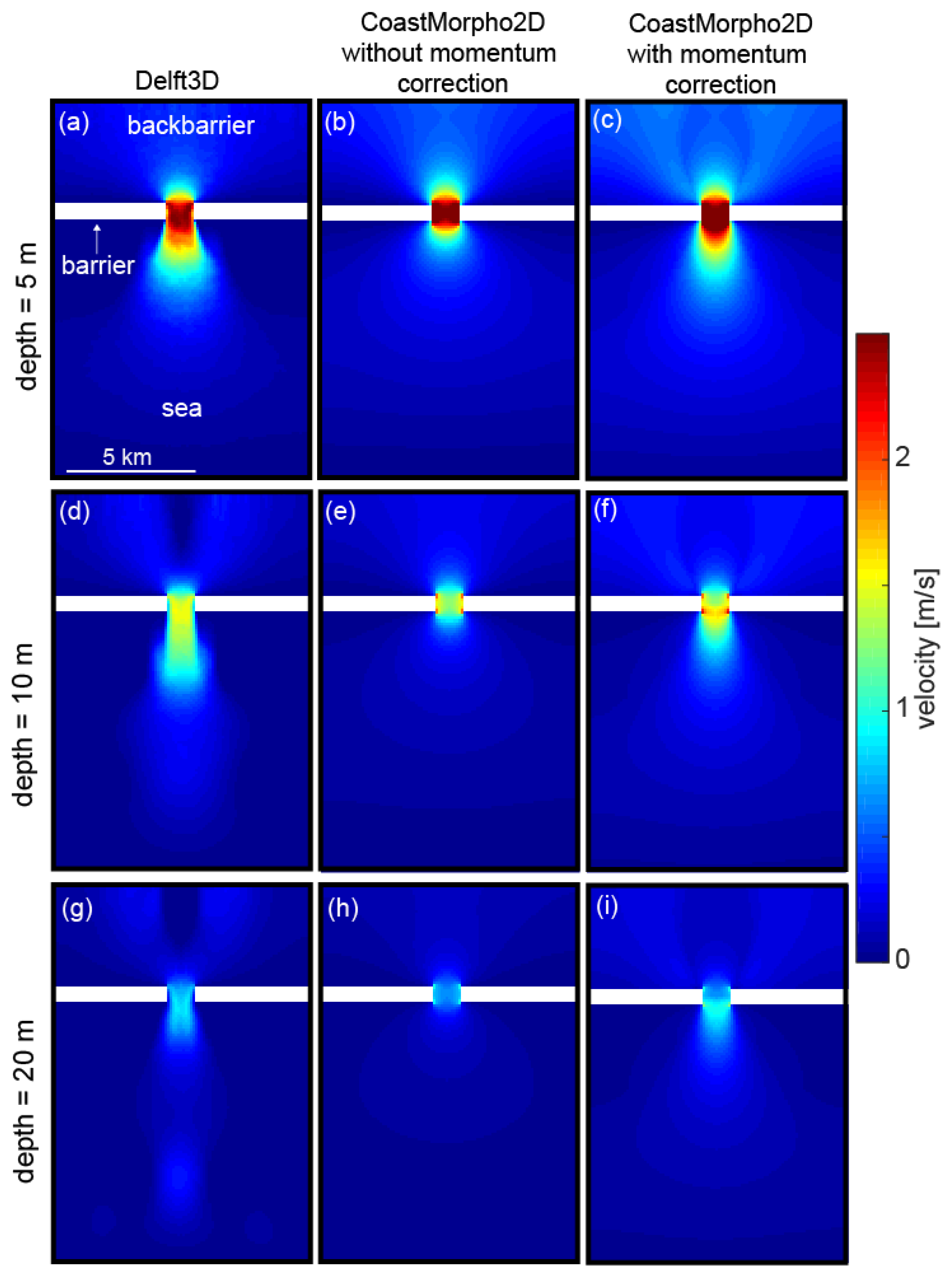
The hydrodynamic comparison is performed on a domain with uniform bed elevation equal to either 5, 10, or 20 m (Figure 2). The domain has two elongated impermeable structures (barrier islands) that create a 1 km wide inlet and separate the backbarrier from the open sea. A sinusoidal water level with a range of 2 m and a period of 12 h (i.e., a semidiurnal tide) is imposed at the seaward boundary of the domain.
The morphodynamic comparison is performed on a domain similar to that used in previous studies [1,6]: a semi-circular basin 16 km wide and 8 km long, connected through a 3 km wide inlet to the open sea (Figure 3). The backbarrier basin has a uniform slope, which leads to a water depth of 3 m at the inlet. The cross-shore profile follows the Dean’s profile and reach 10 m depth at 10 km form the shoreline. A normally distributed elevation with a standard deviation of 0.1 m is added to the whole domain. As for the CM2D model, the total sediment transport is calculated with the Engelund-Hansen formula. In Delft3D, the factor for transverse bedload transport is set equal to 5, and a factor for dry cell erosion equal to 1. Median grain size is set equal to 250 μm.
3. Results
3.1. Hydrodynamics
The hydrodynamic module of CM2D has only one parameter to calibrate: the step to smooth the flow field associated with the advection of momentum (Equation (3)). The best match is found with a smoothing step of 10 m2 in the along flow direction and a smoothing step of 1 m2 in the transverse flow direction (Figure 2).
By refining the spatial resolution to 50 m and 25 m, it is shown that the procedure to calculate the final flow V (which includes both the friction-dominated flow and the correction for the inertial term) does not depend on the spatial resolution (Figure 4).
3.2. Morphodynamics
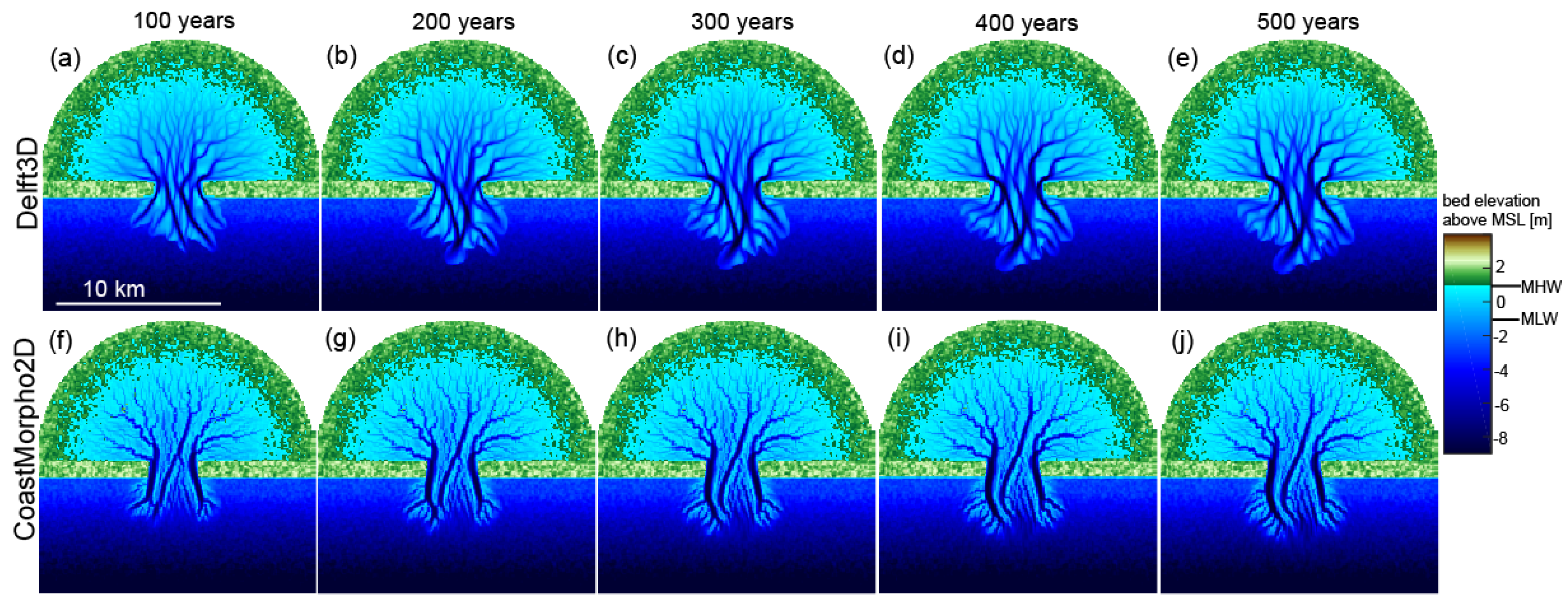
Delft3D reproduces the evolution of the channel network in the backbarrier (Figure 5a–e), which develops mostly during the first hundred years. During the first hundred years a channel network form in the backbarrier basin. The inlet deepens and is dissected by a few large channels. An ebb tidal delta forms offshore. The results are analogous to those obtained from other tide-resolving models [1], even though the details of the channels, especially in the ebb delta, are different.
The CM2D model has two parameters to calibrate for the morphodynamics: the tidal dispersion coefficient (αs) and the downslope transport coefficient (μ). The best match in terms of sediment volume eroded and channel geometry was found using a dispersion coefficient equal to 1 and a downslope coefficient equal to 15. With these parameters the CM2D model qualitatively reproduces the results of Delft3D (Figure 5f–j). The temporal evolution over the first 500 years is similar to that predicted by Delft3D: most of the morphological changes occur during the first hundred years, and only minor changes take place after. Between year 200 and 500 the larger channels tend to deepen by a few meters, reaching maximum depths of about 10 m.
Hypsometry is calculated to give a more quantitative comparison between the two models (Figure 6). In the backbarrier basin the channels reproduced by CM2D are deeper and the intertidal area is higher than in Delft3D (i.e., in CM2D there is a larger portion of elevation between 0.5 and 1 m above MSL). In the ebb delta the hypsometry between the two models matches better, even though the number of channels in the CM2D is smaller than in Delft3D.
3.3. Sensitivity Analysis
The model sensitivity was also tested for temporal and spatial discretization (Figure 7). The temporal resolution (the maximum time step attempted during the morphodynamic update) has a negligible effect on the results, thus justifying the choice of a large time step (2 years). Increasing the spatial resolution to 50 m tends to create a smoother planar configuration of the channels, especially channels with small widths, as previously found with tide-resolving models [1]. Further increasing the spatial resolution (25 m) produces only marginal changes.
Including residual currents in the sediment transport (Equations (11) and (14)) slightly affects the morphology of the ebb delta but not the backbarrier. The largest channels in the ebb delta have a slightly different configuration, especially at the seaward end, but overall have a similar width and depth (Figure 8c). Similarly, removing the correction for the inertial term in the momentum equation (Equation (4))—and thus removing the correction in the reference velocity (Equation (9))—leaves the backbarrier nearly unchanged but causes noticeable changes in the ebb delta (Figure 8b). Specifically, the largest channels tend to bend toward the sides of the inlet, whereas with the inertial terms the largest channels are more aligned perpendicular to the shoreline and extend farther offshore (Figure 8a).
A sensitivity analysis to the morphodynamic parameters shows that greater (smaller) downslope coefficients tend to make shallower (deeper) and wider (narrower) channels, especially in the inlet and ebb delta (Figure 8d,e). A larger (smaller) dispersion coefficient tends to make deeper (shallower) channels, without modifying much the channel width (Figure 8f,g). Also, a larger (smaller) tidal dispersion tends to transport sediment farther (less) offshore.
To test the robustness of the model we also considered the case with a smaller initial inlet: 1.5 km instead of 3 km (Figure 9). In both Delft3D and CM2D, two large channels form at the side of the inlet, which tends to slightly widen. The ebb delta simulated by CM2D is however smaller than the ebb delta predicted with Delft3D.
The CM2D model is also tested for different grain size. With coarser sediment (d50 = 500 μm) the model creates smaller ebb deltas and narrower channels (Figure 10a–d). With finer sediment (d50 = 125 μm) the model creates larger ebb deltas and wider channels (Figure 10e–h). Both results are in accordance with the trends reproduced by Delf3D.
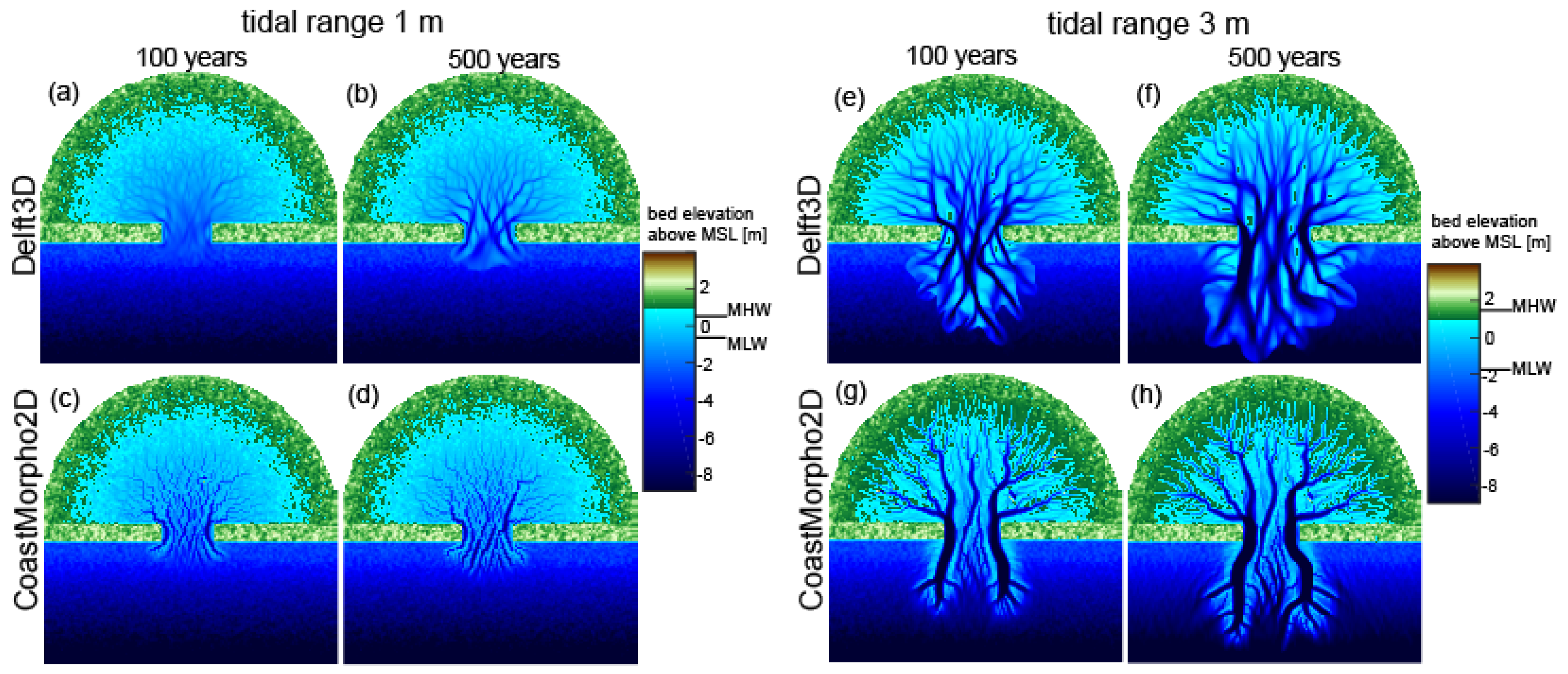
Finally, the influence of tidal range is explored (Figure 11). For a tidal range of 1 m the backbarrier basin develops and ephemeral channel network and the ebb delta extend only 1–2 km offshore. For this tidal range the comparison between Delft3D and CM2D is excellent (Figure 11a–d). For a tidal range of 3 m CM2D predicts a very large ebb delta that extends by about 10 km offshore. The size of the ebb delta is similar to that predicted by Delft3D, but the channel geometry is remarkably different: CM2D creates two major channels with few bifurcations, while Delf3D reproduce a larger number of large channels. Also, CM2D predicts a lower number of channels in the backbarrier than the Delft3D predictions (Figure 11e–h).
3.4. Considerations about the Numerics
A simulation of 500 equivalent years (as in Figure 5) takes about 180 s on a 3.6 GHz single core processor. For comparison, the same simulation using Delft3D takes about 125 days if no morphological acceleration factor is used, and about 6 h with an acceleration factor equal to 500, which is close to the largest value admissible in morphodynamic simulations.
Being the numerical solver implicit, a higher spatial resolution does not require to decrease the time step (while keeping the same threshold for the morphological update). The computation time thus increases close to being linear with the number of cells: 180 s with 25,826 cells (dx = 100 m), 810 s with 102,761 cells (dx = 50 m), and 4220 s with 410,550 cells (dx = 25 m).
4. Discussion
4.1. Hydrodynamics, Jet Dynamics, and Residual Currents
The hydrodynamics model captures the main features of the jet-flow during the ebb phase of the tide (Figure 2). For different basin depths the magnitude of the peak tidal flow is within 10% of that given by the tide-resolving model (Delft3D). The simulated jet, however, does not extend as far as in Delf3D. This difference highlights the limit of the semi-empirical correction, which only uses the values from the friction-dominated flow (Figure 2b,e,h). An iterative solution might provide a jet-like flow that extends farther offshore, but this could increase the computation time and is thus not pursued.
The momentum correction helps to direct the flow and the sediment accumulation in front of the inlet (Figure 2c,f,i). Without this correction the flow does not extend far from the inlet (Figure 2b,e,h), and the ebb delta does not have a depocenter in front of the inlet but rather on the sides (Figure 8c). It is however surprising that elongated channels can form even without the correction for the inertial term (Figure 8c). Specifically, the channels extend farther than expected by considering the weak flow field associated with the initial configuration (Figure 2b,e,h). This result suggests that the flow within the channels is strongly driven by the channel geometry, which forces the flow to be concentrated in the channels and to extend far from the inlet even without the inertial term. This mechanism resembles the topographic steering in channel bends [24], where outward velocity displacement is forced directly by the geometry of the channel bend rather by the secondary circulation (i.e., by a direct hydrodynamic effect). It is thus possible that strong morphodynamic feedbacks might suffice to create realistic morphodynamic features in ebb deltas, thus justifying the use of a simple representation for flow redistribution.
We also notice that the largest morphodynamic consequence of the inertial correction is to modify the effective velocity (and thus the erosion term, Equation (9)) rather than to create residual transport (Equation (14)). Indeed, the introduction of the residual currents associated with the ebb-flood asymmetry determines relatively small changes to the ebb delta (compare Figure 8a,b), as opposed to the effect of removing the inertial correction from the effective velocity (compare Figure 8a,c).
4.2. Morphodynamics
The parameterization of the downslope transport strongly affects the width to depth ratio of the channels. This result confirms a previous sensitivity analysis performed with Delft3D [4], which showed that the factor for transverse bedload transport (which is analogous to the downslope parameter μ) controls the channel width to depth ratio. In Delft3D, channel widening could also be enhanced by increasing the dry-cell erosion factor [25]. This method is actually necessary in Delft3D to allow for widening of the inlet (Figure 9), whose banks cannot be eroded directly by bed shear stress (i.e., the term E). Contrary, CM2D does not require such technique to erode dry cells (i.e., the banks). Indeed, in the finite volume method, the downslope flux is calculated averaging the downslope term S between the wet and dry cells, which automatically allows us to transport material from the dry cell to the wet cell. A similar downslope sediment transport has been previously employed to simulate tidal morphodynamics [6,23], but we are not aware of any model in which this mechanism was successfully used to reproduce bank erosion (i.e., to enlarge channels with dry banks).
The channel network that develops in the backbarrier is similar for Delft3D and CM2D. This is not surprising, given that the ability of the tidal dispersion model to simulate the backbarrier (lagoon) environment was previously shown [12]. We however notice that CM2D predicts a larger amount of area between mean sea level and high tide level than Delft3D, suggesting that the model does not perform well in the upper intertidal zone. This effect might be linked to the use of a depth-averaged method, which is less accurate where water depths are small. On the other hand, this effect might be canceled by the effect of wind waves, which would tend to preferentially erode the shallow part of the backbarrier [12]. Indeed, the overestimation of the height of the intertidal areas was not present in a tidal dispersion model that included wind waves [12].
The ebb delta predicted by CM2D has less, more distinct, wider channels compared to Delft3D predictions, which instead predicts a larger number of narrower channels that intersect with each other (Figure 5e,j). The smaller number of channels in CM2D is probably due to the diffusive nature of the sediment transport model, which tends to limit incision of smaller channels where the rate of sediment transport is high. These differences are however not so large if put into a larger perspective. Indeed, it is well established that even models that solve the same equations (with the same spatial resolution) but with different numerical schemes give quantitatively different results, especially in the ebb delta region [1].
One reason why the CMSD model is able to reproduce the major morphological features is that, despite simplified, the model conserves the sediment mass (up to the machine precision). The model is thus forced to transfer the sediment eroded from the backbarrier to the nearshore region, where an ebb delta must form. In other words, mass conservation might impose the largest constraint on coastal evolution over long time scales. In this sense, the model is similar to an aggregated model such as ASMITA [26], which moves sediment between compartments while conserving the total mass. In CM2D this sediment redistribution is obtained through a very simplified hydrodynamics. By calibrating the dispersion and downslope transport, CM2D produces morphological features that are very close to those obtained with more sophisticated models.
We also emphasize that the morphodynamics has only two calibration parameters: the dispersion coefficient and the downslope transport coefficient. The model results might be improved by including ad hoc modifications of the formulas for erosion, dispersion, and downslope transport. For example, the sediment transport equation (Equation (8)) might be multiplied by some functions of water depth or velocity to phenomenologically recreate a more realistic channel network, i.e., an ebb delta with more channels.
4.3. Model Limitations and Future Directions
Despite capturing the major features, the model does not reproduce some fine details of the morphodynamics. Thus, the model should not be used for short-term (<50 years) engineering predictions. Its ability to conserve sediment makes it suitable for long term simulations, possibly with the inclusion of sea level rise. Thus, the model should be considered as a complement to rather than a substitute for Delft3D (or for a similar high-resolution model).
Several processes could be added to the model to make it more realistic. As previously discussed, locally generated wind waves might be important in the backbarrier area where water depths are small. These can be easily be implemented as done by Di Silvio et al. [12], or by including a simplified wind wave model that depends both depth and fetch [27,28]. Marsh dynamics can be included following previous approaches that parameterize organic sediment production, drag, and sediment trapping [29]. Marsh edge erosion by wind waves can be simulated with simplified probabilistic algorithms [30]. River flow can be added using simplified models, for example coupling the CM2D model with a reduced complexity model for delta evolution [31]. A more realistic reproduction of the shoreface would require us to include swell waves. A simplified approach, for example a spectral model that only considers wave propagation in the half plane [32], might provide a tool with a computation cost comparable to that of the hydrodynamic model.
In line with previous studies [1,3,4,5,6,7,8,9], CM2D neglected the presence of multiple sediment classes. This simplification allowed us to directly compare the newly developed CM2D model to previous studies based on tide-resolving models. This simplification does however limit the applicability of the model to the real world. Mud can indeed control the filling and emptying of tidal basins [30], and could lead to the formation of salt marshes. Future model developments should thus consider the coupled dynamics of sand-mud dynamics and the associated stratigraphy.
Future efforts should also try to compare the CM2D predictions to field data, especially after the processes mentioned above are added to the model. Given the nature of the model, comparisons would be best achieved by considering long term datasets, e.g., by comparing historical (>100 years) topobathymetric maps. In general, the model is more likely to be successful at reproducing large scale and long-term changes than fine-scale changes.
5. Conclusions
Here we described a simple morphodynamic model that further expands upon the concept of tidal dispersion [12]. A novel semi-empirical correction for the inertial term in the momentum equation was introduced, allowing to calculate jet-like flow and residual currents. These currents were however not found to be crucial for the morphodynamics. Comparison with a tide-resolving model showed that the simplified model can simulate non-cohesive sediment (sand) transport and morphodynamics in both backbarrier and nearshore environments. The model is especially effective in simulating a large window of tidal ranges. With opportune calibration of the dispersion and downslope transport, the model reproduces the main features of the backbarrier tidal network as well as the ebb tidal delta. This validation suggests that the model might be used to predict long-term and large-scale coastal changes.
Author Contributions
Conceptualization, G.M.; Methodology, G.M.; Software, G.M. and S.M.; Validation, G.M. and S.M.; Formal Analysis, G.M.; Investigation, G.M.; Resources, G.M.; Data Curation, G.M.; Writing-Original Draft Preparation, G.M.; Writing-Review & Editing, G.M.; Visualization, G.M.; Supervision, G.M.; Project Administration, G.M.; Funding Acquisition, G.M.
Funding
This research received no external funding.
Conflicts of Interest
The authors declare no conflict of interest.
References
- Coco, G.; Zhou, Z.; van Maanen, B.; Olabarrieta, M.; Tinoco, R.; Townend, I. Morphodynamics of tidal networks: Advances and challenges. Mar. Geol. 2013, 346, 1–16. [Google Scholar] [CrossRef]
- Elko, N.; Feddersen, F.; Foster, D.L.; Holman, R.A.; McNinch, J.; Ozkan-Haller, H.T.; Plant, N.G.; Raubenheimer, B.; Elgar, S.; Hay, A.E.; et al. The Future of Nearshore Processes Research. In Proceedings of the 2014 Fall Meeting, San Francisco, CA, USA, 15–19 December 2014; AGU: Washington, DC, USA, 2014; p. OS22A-08. [Google Scholar]
- Dissanayake, D.M.P.K.; Ranasinghe, R.; Roelvink, J.A. The morphological response of large tidal inlet/basin systems to relative sea level rise. Clim. Chang. 2012, 113, 253–276. [Google Scholar] [CrossRef] [Green Version]
- Dissanayake, D.M.P.K.; Roelvink, J.A.; van der Wegen, M. Modelled channel patterns in a schematized tidal inlet. Coast. Eng. 2009, 56, 1069–1083. [Google Scholar] [CrossRef]
- van Maanen, B.; Coco, G.; Bryan, K.R.; Friedrichs, C.T. Modeling the morphodynamic response of tidal embayments to sea-level rise. Ocean Dyn. 2013, 63, 1249–1262. [Google Scholar] [CrossRef]
- van Maanen, B.; Coco, G.; Bryan, K.R. Modelling the effects of tidal range and initial bathymetry on the morphological evolution of tidal embayments. Geomorphology 2013, 191, 23–34. [Google Scholar] [CrossRef]
- Dissanayake, D.M.P.K.; Ranasinghe, R.; Roelvink, J.A. Effect of Sea Level Rise in Tidal Inlet Evolution: A Numerical Modelling Approach. J. Coast. Res. 2009, II, 942–946. [Google Scholar]
- van Leeuwen, S.M.; van der Vegt, M.; de Swart, H.E. Morphodynamics of ebb-tidal deltas: A model approach. Estuar. Coast. Shelf Sci. 2003, 57, 899–907. [Google Scholar] [CrossRef]
- Ridderinkhof, W.; de Swart, H.E.; van der Vegt, M.; Hoekstra, P. Influence of the back-barrier basin length on the geometry of ebb-tidal deltas. Ocean Dyn. 2014, 64, 1333–1348. [Google Scholar] [CrossRef]
- Lesser, G.R.; Roelvink, J.A.; van Kester, J.A.T.M.; Stelling, G.S. Development and validation of a three-dimensional morphological model. Coast. Eng. 2004, 51, 883–915. [Google Scholar] [CrossRef]
- Dal Monte, L.; Di Silvio, G. Sediment concentration in tidal lagoons. A contribution to long-term morphological modelling. J. Mar. Syst. 2004, 51, 243–255. [Google Scholar] [CrossRef]
- Di Silvio, G.; Dall’Angelo, C.; Bonaldo, D.; Fasolato, G. Long-term model of planimetric and bathymetric evolution of a tidal lagoon. Cont. Shelf Res. 2010, 30, 894–903. [Google Scholar] [CrossRef]
- Bonaldo, D.; Di Silvio, G. Historical evolution of a micro-tidal lagoon simulated by a 2-D schematic model. Geomorphology 2013, 201, 380–396. [Google Scholar] [CrossRef]
- Özsoy, E.; Ünlüata, Ü. Ebb-tidal flow characteristics near inlets. Estuar. Coast. Shelf Sci. 1982, 14, 251–263. [Google Scholar] [CrossRef]
- Spearman, J. The development of a tool for examining the morphological evolution of managed realignment sites. Cont. Shelf Res. 2011, 31, S199–S210. [Google Scholar] [CrossRef]
- Gatto, V.M.; van Prooijen, B.C.; Wang, Z.B. Net sediment transport in tidal basins: Quantifying the tidal barotropic mechanisms in a unified framework. Ocean Dyn. 2017, 67, 1385–1406. [Google Scholar] [CrossRef]
- Mariotti, G. Marsh channel morphological response to sea level rise and sediment supply. Estuar. Coast. Shelf Sci. 2018, 209, 89–101. [Google Scholar] [CrossRef]
- Tambroni, N.; Seminara, G. Are inlets responsible for the morphological degradation of Venice Lagoon? J. Geophys. Res. Earth Surf. 2006, 111. [Google Scholar] [CrossRef] [Green Version]
- Engelund, F.; Hansen, E. A Monograph on Sediment Transport in Alluvial Streams; Tekniskforlag Skelbrekgade 4 Copenhagen V Denmark: Copenhagen, Denmark, 1967. [Google Scholar]
- Arons, A.B.; Stommel, H. A mixing-length theory of tidal flushing. Eos Trans. Am. Geophys. Union 1951, 32, 419–421. [Google Scholar] [CrossRef]
- Zimmerman, J.T.F. Mixing and flushing of tidal embayments in the Western Dutch Wadden Sea, part II: Analysis of mixing processes. Neth. J. Sea Res. 1976, 10, 397–439. [Google Scholar] [CrossRef]
- Geyer, W.R.; Signell, R.P. A Reassessment of the Role of Tidal Dispersion in Estuaries and Bays. Estuaries 1992, 15, 97–108. [Google Scholar] [CrossRef]
- Cayocca, F. Long-term morphological modeling of a tidal inlet: The Arcachon Basin, France. Coast. Eng. 2001, 42, 115–142. [Google Scholar] [CrossRef]
- Dietrich, W.E.; Smith, J.D. Influence of the point bar on flow through curved channels. Water Resour. Res. 1983, 19, 1173–1192. [Google Scholar] [CrossRef]
- Dissanayake, P.K. Modelling Morphological Response of Large Tidal Inlet Systems to Sea Level Rise UNESCO-IHE PhD Thesis; CRC Press: Boca Raton, FL, USA, 2011; ISBN 978-1-4665-5280-7. [Google Scholar]
- Van Goor, M.A.; Zitman, T.J.; Wang, Z.B.; Stive, M.J.F. Impact of sea-level rise on the morphological equilibrium state of tidal inlets. Mar. Geol. 2003, 202, 211–227. [Google Scholar] [CrossRef]
- Fagherazzi, S.; Wiberg, P.L. Importance of wind conditions, fetch, and water levels on wave-generated shear stresses in shallow intertidal basins. J. Geophys. Res.-Earth Surf. 2009, 114. [Google Scholar] [CrossRef] [Green Version]
- Mariotti, G.; Fagherazzi, S. Wind waves on a mudflat: The influence of fetch and depth on bed shear stresses. Cont. Shelf Res. 2013, 60, S99–S110. [Google Scholar] [CrossRef]
- Fagherazzi, S.; Kirwan, M.L.; Mudd, S.M.; Guntenspergen, G.R.; Temmerman, S.; D’Alpaos, A.; van de Koppel, J.; Rybczyk, J.M.; Reyes, E.; Craft, C.; et al. Numerical models of salt marsh evolution: Ecological, geomorphic, and climatic factors. Rev. Geophys. 2012, 50, RG1002. [Google Scholar] [CrossRef]
- Mariotti, G.; Canestrelli, A. Long-term morphodynamics of muddy backbarrier basins: Fill in or empty out? Water Resour. Res. 2017, 53, 7029–7054. [Google Scholar] [CrossRef]
- Liang, M.; Voller, V.R.; Paola, C. A reduced-complexity model for river delta formation—Part 1: Modeling deltas with channel dynamics. Earth Surf. Dyn. 2015, 3, 67–86. [Google Scholar] [CrossRef]
- Smith, J.M.; Sherlock, A.R.; Resio, D.T. STWAVE: Steady-State Spectral Wave Model: User’s Manual for STWAVE Version 3.0; Supplemental Report ERDC/CHL SR-01-1; U.S. Army Engineer Research and Development: Saint Louis, MO, USA, 2001. [Google Scholar]
Figure 1.
Scheme of the CM2D model, including both hydrodynamic and morphodynamic processes. The red text highlights the sediment transport mechanisms.
Figure 1.
Scheme of the CM2D model, including both hydrodynamic and morphodynamic processes. The red text highlights the sediment transport mechanisms.

Figure 2.
Hydrodynamic comparison between Delft3D and CM2D. Both models simulate the flow from a basin to an open sea through an idealized inlet. The bed elevation is uniform in the domain and is set equal to either 5 m (a–c), 10 m (d–f), or 20 m (g–i). The white rectangles indicate impermeable barriers, which defines a 1 km wide inlet. The tidal range is 2 m. The plots shows velocity field during peak ebb flow for both Delft3D and CM2D. (a,d,g) Delft3D; (b,e,h) Hydrodynamic model without correction for momentum advection (i.e., the flow field U); (c,f,i) Hydrodynamic model with correction for momentum advection (i.e., the flow field W).

Figure 3.
Initial model bathymetry and boundary conditions.

Figure 4.
Sensitivity analysis reproducing the peak ebb flow for the idealized basin geometry with a depth of 10 m (as in Figure 2f) using a spatial discretization (dx) equal to (a) 100 m; (b) 50 m; and (c) 25 m.
Figure 4.
Sensitivity analysis reproducing the peak ebb flow for the idealized basin geometry with a depth of 10 m (as in Figure 2f) using a spatial discretization (dx) equal to (a) 100 m; (b) 50 m; and (c) 25 m.

Figure 5.
Reference simulations with Delft3D and with CM2D with best fit parameters. (a–e) Delft3D, plotted every 100 years; (f–j) CM2D, plotted every 100 years.
Figure 5.
Reference simulations with Delft3D and with CM2D with best fit parameters. (a–e) Delft3D, plotted every 100 years; (f–j) CM2D, plotted every 100 years.

Figure 6.
Comparison of hypsometry in the backbarrier basin (a) and in the ebb delta (b) at year 500 (Figure 5e,j).
Figure 6.
Comparison of hypsometry in the backbarrier basin (a) and in the ebb delta (b) at year 500 (Figure 5e,j).

Figure 7.
Sensitivity analysis of CM2D with respect to spatial and temporal resolution. All simulations are compared at year 500 (Figure 5e). (a) Reference simulation with a spatial resolution of 100 m and maximum time step of 2 years; (b,c) Maximum time step equal to 1 and 0.5 years; (d,e) Spatial resolution equal to 50 and 25 m.

Figure 8.
Sensitivity analysis of CM2D with respect to different parameters. All simulations are compared at year 500 (Figure 5e). (a) Reference scenario (as in Figure 5e); (b) Scenario in which the residual currents (Equation (14)) are included in the sediment transport (Equation (11)); (c) Scenario without the correction for the inertial term (Equation (4)) in the hydrodynamic model (Equations (2) and (3)); (d,e) Scenarios with different values of the downslope coefficient; (f,g) Scenarios for different values of the tidal dispersion coefficient.


Figure 9.
Comparison between Delft3D and CM2D for the reference case (as in Figure 5e), but with an initial inlet width of 1.5 km instead of 3 km. (a) Initial configuration; (b,c) Results with Delft3D at year 100 and 500; (d,e) Results with CM2D at year 100 and 500.
Figure 9.
Comparison between Delft3D and CM2D for the reference case (as in Figure 5e), but with an initial inlet width of 1.5 km instead of 3 km. (a) Initial configuration; (b,c) Results with Delft3D at year 100 and 500; (d,e) Results with CM2D at year 100 and 500.

Figure 10.
Comparison between Delft3D and CM2D for different sediment grain size. Simulations are compared at year 500 with the reference parameters (Figure 5e). (a–d) Median grain size equal to 500 μm; (e–h) Median grain size equal to 125 μm.
Figure 10.
Comparison between Delft3D and CM2D for different sediment grain size. Simulations are compared at year 500 with the reference parameters (Figure 5e). (a–d) Median grain size equal to 500 μm; (e–h) Median grain size equal to 125 μm.

Figure 11.
Comparison between Delft3D and CM2D for different tidal ranges. Simulations are compared at year 500 with the reference parameters (Figure 5e). (a–d) Tidal range equal to 1 m; (e–h) Tidal range equal to 1 m. Note the change in the MHW and MLW levels on the elevation scale.
Figure 11.
Comparison between Delft3D and CM2D for different tidal ranges. Simulations are compared at year 500 with the reference parameters (Figure 5e). (a–d) Tidal range equal to 1 m; (e–h) Tidal range equal to 1 m. Note the change in the MHW and MLW levels on the elevation scale.


Table 1.
Reference parameters used in the model CM2D.
| Parameter | Description | Value | Source |
|---|---|---|---|
| r | Astronomic tidal range | 2 m | fixed |
| n | Manning friction coefficient | 0.02 m−1/3s | fixed |
| d50 | Median grain size | 250 μm | fixed |
| ρbulk | Sediment dry bulk density | 1600 kg/m3 | fixed |
| γ | Water density | 1030 | fixed |
| T | Tidal period | 12 h | fixed |
| Δt | Maximum time step | 2 year | fixed |
| Δx | Spatial resolution | 100 m | fixed |
| Diffusion step for momentum correction in the along-flow direction | 10 m2 | calibrated | |
| Diffusion step for momentum correction in the transverse-flow direction | 1 m2 | calibrated | |
| αs | Tidal dispersion coefficient | 1 | calibrated |
| μ | Coefficient for downslope sediment transport | 15 | calibrated |
© 2018 by the authors. Licensee MDPI, Basel, Switzerland. This article is an open access article distributed under the terms and conditions of the Creative Commons Attribution (CC BY) license (http://creativecommons.org/licenses/by/4.0/).
Share and Cite
MDPI and ACS Style
Mariotti, G.; Murshid, S. A 2D Tide-Averaged Model for the Long-Term Evolution of an Idealized Tidal Basin-Inlet-Delta System. J. Mar. Sci. Eng. 2018, 6, 154. https://doi.org/10.3390/jmse6040154
AMA Style
Mariotti G, Murshid S. A 2D Tide-Averaged Model for the Long-Term Evolution of an Idealized Tidal Basin-Inlet-Delta System. Journal of Marine Science and Engineering. 2018; 6(4):154. https://doi.org/10.3390/jmse6040154
Chicago/Turabian StyleMariotti, Giulio, and Shamim Murshid. 2018. "A 2D Tide-Averaged Model for the Long-Term Evolution of an Idealized Tidal Basin-Inlet-Delta System" Journal of Marine Science and Engineering 6, no. 4: 154. https://doi.org/10.3390/jmse6040154
Note that from the first issue of 2016, this journal uses article numbers instead of page numbers. See further details here.