Storm Surge Propagation and Flooding in Small Tidal Rivers during Events of Mixed Coastal and Fluvial Influence


Pacific Coastal and Marine Science Center, United States Geological Survey, Santa Cruz, CA 95060, USA
*
Author to whom correspondence should be addressed.
J. Mar. Sci. Eng. 2018, 6(4), 158; https://doi.org/10.3390/jmse6040158
Submission received: 28 September 2018
/
Revised: 5 November 2018
/
Accepted: 12 November 2018
/
Published: 17 December 2018
(This article belongs to the Special Issue Selected Papers from the 15th Estuarine and Coastal Modeling Conference)
Abstract
:The highly urbanized estuary of San Francisco Bay is an excellent example of a location susceptible to flooding from both coastal and fluvial influences. As part of developing a forecast model that integrates fluvial and oceanic drivers, a case study of the Napa River and its interactions with the San Francisco Bay was performed. For this application we utilize Delft3D-FM, a hydrodynamic model that computes conservation of mass and momentum on a flexible mesh grid, to calculate water levels that account for tidal forcing, storm surge generated by wind and pressure fields, and river flows. We simulated storms with realistic atmospheric pressure, river discharge, and tidal forcing to represent a realistic joint fluvial and coastal storm event. Storm conditions were applied to both a realistic field-scale Napa river drainage as well as an idealized geometry. With these scenarios, we determine how the extent, level, and duration of flooding is dependent on these atmospheric and hydrologic parameters. Unsurprisingly, the model indicates that maximal water levels will occur in a tidal river when high tides, storm surge, and large fluvial discharge events are coincident. Model results also show that large tidal amplitudes diminish storm surge propagation upstream and that phasing between peak fluvial discharges and high tide is important for predicting when and where the highest water levels will occur. The interactions between tides, river discharge, and storm surge are not simple, indicating the need for more integrated flood forecasting models in the future.
1. Introduction
Coastal and inland flooding damage property and endanger lives, with the losses from inland flooding averaging $7.96 billion in damages and 82 fatalities per year over the 30 years prior to 2014, in the United States alone [1]. Inland and coastal flooding are expected to worsen in the future. Many locations (including the US) around the world are experiencing increases in heavy precipitation events, with this trend expected to accelerate with climate change [2]. Coastal flooding is becoming more frequent and expensive with sea level rise (SLR). Studies show that in the future there will be increases in the frequency of nuisance flooding [3], and that flooding frequencies will double in decades in some locations from both SLR and storm and wave frequency changes [4]. More frequent flooding will have significant socioeconomic impacts. In coastal regions near rivers, such as San Francisco Bay, both fluvial-driven flooding and oceanic flooding can cause significant damage. Events like the winter storms in February 1998 (part of an El Ni͠ño weather pattern) caused 9 m waves off the coast of California and large rainfall in coastal watersheds, both of which caused flooding [5]. This weather pattern is an example of one storm that can be the cause of both coastal and fluvial flooding, and there is evidence that this occurs for smaller storm systems as well. The changing nature of these events with climate change makes it necessary to have both short-term and long-term predictive models for these floods.
The economic impacts of coincident flooding can be exacerbated by the fact that historical settlement patterns have favored settlement along rivers in locations where coastal/tidal dynamics still play a role. This zone of mixed fluvial and coastal influences was a good place to settle since it often represents a location with access to fresh water, rich estuarine food resources, and a navigable channel [6]. However, the benefits of being in a zone of mixed fluvial and coastal influence mean that it is susceptible to flooding from both coastal and fluvial causes. This paper focuses on the Napa River watershed which is emblematic of this development pattern as the downtown of the largest city in the region is located at the head of the tide in the river. Traditionally, there is not a significant amount of communication between the agencies responsible for flood prediction on the coast and those that predict flooding in rivers. Most forecast models that are currently in use do not incorporate the forcings necessary to represent these mixed events. Separation of these communities is evident in that, there are many papers on coastally driven flooding (e.g., [7,8]) and many papers on fluvial flooding (e.g., [9]) but relatively few that consider the compound impact of the two. Given the concentration of people residing in these regions, our aim is to better understand these compound flooding events and understand the utility of short-term predictive models for these types of events.
While storm events have not been specifically studied, the dynamics of rivers with coastal influence have been studied, especially, with regard to the interactions of tidal propagation in rivers. LeBlond [10] found that in the tidally influenced St Lawrence river, the main momentum balance was between friction and the free surface gradient except during the brief periods of slack tide when velocity and thus the friction term becomes zero leaving the unsteady inertia term to balance the free surface gradient. LeBlond [11] also reported that the subtidal wave (i.e., spring-neap variability) is amplified as it progresses upstream. Work in other large rivers like the Amazon ([12,13], Yangtze [14,15,16], and Columbia Rivers [17,18] has made similar findings, indicating that spring-neap variations penetrate farther upstream in a tidal river than the daily tidal oscillation. These rivers differ from the varied small tributaries in San Francisco Bay in that they are much larger in width and depth, have larger flow rates, and the region of tidal influence extends for hundreds of km upstream of the coast instead of tens of kilometers. In these larger rivers, understanding the physics of variable discharges has been pursued by frequency-based analysis because the large basins create discharge hydrographs that occupy distinct frequency space from that of the tidal motions. For example, Sassi and Hoitink [19] found that the tidal damping that occurs during the rising limb is different from the damping that occurs during the falling limb of a discharge curve. In smaller rivers with typical hydrograph durations near the dominant tidal frequency (12.42 h) it is not clear if the duration of the discharge relative to the tidal phase is long enough to produce similar interactions.
Storm surge has been widely studied but primarily with a focus on coastal areas, not extending farther up into rivers. A number of factors contribute to storm surge, including atmospheric pressure gradients, wind speed [20], and storm propagation speed [21]. The local bathymetry and land use also plays an important role in predicting local water levels. Sabatino et al. [22] found that funneling can create higher storm surges as one progresses up a narrowing estuary. Land use changes such as wetland restorations can also have an important impact on total water levels in storm surge propagation [23,24]. Condon and Sheng [25] found that coastal inundation predicted by sea level rise creates an overestimate in flooding relative to the same water level increase from storm surge because land dissipation is neglected. A similar result was found by Wang et al., [26] who showed that a storm surge of short enough duration can dissipate before reaching the maximum inland water levels. All of these studies find that once atmospheric forcing sets the storm surge coastal water levels, the propagation in inland bays and channels is primarily affected by interaction with local bathymetry and topography. Few studies extend the domain to include the propagation of storm surge up smaller river channels, likely because it requires a significant change in the model resolution.
The work that has been done considering the compound effects of tides, storm surge, and fluvial discharge has found that timing is a complicating factor in understanding the severity of coastal storms and rainfall-induced flooding. The timing of the arrival of the peak of the storm hydrograph to the coastal region is influenced by the spatial distribution of the rain in the watershed, and the shape, size, slope, soil type, and level of urbanization in the watershed [27]. The storm surge is linked via the fact that it is primarily driven by atmospheric forcing (wind and pressure) which is linked to the distribution of rainfall. Occurring separately from the storm are the astronomical tides that can also drive large variations in coastal water levels. Zheng et al. [27] found that the timing of river discharge phasing relative to tidal forcing is of great importance in predicting total water levels. Moreover, Zheng et al. [28] found that different locations have different probabilistic interdependences between rainfall intensity and storm surge. This interaction of storm surge with fluvial discharge is, of course, more likely to cause flooding in locations where atmospheric forcing and local watershed characteristics create a strong interdependence between coastal wind and pressure and overland rainfall.
In this work, we investigate the dynamics relevant for predicting water levels in smaller tidal rivers for relatively short time-scales and explicitly consider the effects of storm surge in addition to tides. Our primary interest is in how the storm surge changes the flows in the river and resultant flooding from the interaction of oceanic and fluvial drivers. Not only are we examining the impacts of storm surge, but additionally we focus on a smaller river size than has been examined in the past (e.g., Puget Sound WA, US; Chesapeake Bay, MD, US; Severn Estuary, UK; and Moreton Bay, AU). Our focus area is San Francisco Bay, into which numerous small rivers drain and extensive critical infrastructure (roads, airports, wastewater treatment systems) and large populations align the coast and are at risk of mixed oceanic and fluvial flooding. In this paper, we first provide background on the location and relevant physics, then describe our modeling set up and the scenarios. Lastly, we show the relative impacts of each of the forcings: fluvial, tidal, and storm surge, and how their interactions change flooding potentials.
1.1. Study Area: Hydrodynamic Characteristics
San Francisco Bay is an urbanized estuary which opens to the ocean at the narrow mouth of the Golden Gate (37.8° N, 122.5° W) and extends inland to connect to the Sacramento and San Joaquin Delta and rivers. The open coast at the mouth is subject to swell from the entire Pacific Ocean, thus it can be a fairly energetic environment with the mean annual significant wave height () of 2.5 m with the annual maximum typically exceeding 8 m [29]. The water level at the Golden Gate can be raised significantly by the wave conditions as well as global-scale climate patterns like the El Niño Southern Oscillation and the Pacific Decadal Oscillation. The tides at the Golden Gate are mixed semi-diurnal with a diurnal tidal range of 1.78 m (mean lower low water to mean higher high water, MLLW-MHHW). The Bay is at a maximum depth near the opening of the Golden Gate (113 m) and shallows as the channel goes inland to San Pablo Bay (with channel depths of 11 to 24 m). The tidally driven currents range from just above 2 m/s in Central Bay to as high as 1 m/s in the shallower channel reaches [30] The Napa River drains into a narrow straight, between two sub embayments where currents regularly reach 1.5 m/s during peak flood and ebb.
1.2. Study Area: Hydrologic Characteristics
There are 483 watersheds draining into the San Francisco Bay landward of the Golden Gate bridge. Of these, 482 of them are relatively small. The Sacramento and San Joaquin Rivers account for 95% of the total watershed areas that drain into the Bay, with the remaining 482 watersheds accounting for only 5% of the total. Although a small percentage of the total watershed, the many small tributaries are located in the nine urbanized counties and are home to 7.151 million people [31]. The Napa River watershed is among the larger of the remaining 482 watersheds at 1100 km2 and is a mix of urban (9%), agricultural (35%), grassland (15%), and forests (40%) with the area adjacent to the Bay being restored to a wetland habitat. It extends from the Mayacamas Mountains to the north and empties into the Bay west of the Carquinez straight [6]. The watershed is bounded by relatively steep terrain surrounding the long narrow valley that is 43 km long and 8 km wide at its widest point. The city of Calistoga is in the northern end of the watershed and the city of Napa sits at the southern, tidally influenced end, with Vallejo, CA located on the eastern side of the river where it meets the Bay, as shown in Figure 1.
1.3. Study Area: Geology
The Central and San Pablo Bays have been filled since 5 ka with the fringing saltmarshes being developed ~4.7 ka. Over the last two centuries, human activity has significantly altered the sediment system. Gold mining activity led to a deposition of ~350 million m3 of sediment between 1856 and 1887. In the 20th century, dams, reservoirs, flood control bypasses, and bank protection systems have reduced the delivery of sediment to the bay. In the current era, direct sediment removal occurs regularly via dredging, aggregate mining, and borrow pit mining [30].
Current bed conditions vary spatially throughout the bay. The Golden Gate inlet is comprised of bedrock. The strait that the Napa River drains just west of is 35 m deep and flanked by rock. San Pablo Bay has an 11–24 m-deep channel with a mostly sandy bed, whereas 80% of the San Pablo Bay consists of mud-dominated tidal flats [32]. The river channel itself is made up of coarse to fine sands on the bay side with gravel deposits and cobble in the most upstream reaches of the study area. Cohesive alluvial fan sediments, as well as tidally transported cohesive bay muds, flank the river banks. The marsh plains at the mouth of the river have been shown to accrete between 5 to 50 mm/year while the river flood plains accrete 0 to 39 mm/year, with any accretion rates greater than 30 mm/year being extremely localized [33].
1.4. Study Area: Human and Natural Pressures
Historically, the Napa River and the adjacent bay region have been vulnerable to floods from both coastal and fluvial influences. Since 1862, there have been at least 27 flood events on the river with the most recorded damage occurring in February 1986 when 7000 residents were forced to evacuate, resulting in three deaths and $100 million dollars in damage [34]. The most recent flooding along the river occurred in 2017, although it was to a much lesser extent than it might have been without the completion of a major flood project along the river corridor in 2016 at the cost of $565 million dollars. Among other things, this project widened the floodplain and added a flood bypass channel to the oxbow portion of the river, significantly increasing the throughput of water in high-flow conditions and protecting downtown Napa. The flood bypass was designed to maintain the existing energy slope, thus maintaining the longitudinal sediment equilibrium. This project also increased the tidal prism downstream of downtown Napa, decreasing the amount of tidal flow penetration upstream [33].
There is significant infrastructure in these regional floodways, including Highway 37. This highway serves 38,000–40,000 drivers a day [35], crosses the Napa River mouth and follows along the bay shoreline to the north. The highway’s proximity to bay wetlands makes it susceptible to nuisance flooding when there are high coastal water levels. The most recent closure due to flooding was in February 2017 for at least a week [36]. There are also records of at least four other road closures from flooding since 1999, with the longest duration of closure being for 21 days in January 2005 [37]. By the year 2060, there is a 40–65% likelihood that SLR will reach or exceed 30 cm in the bay [38] which would only exacerbate this problem. In some regions of the bay, the effective SLR will be higher due to subsidence and the consolidation of sediments, although this is less of an issue in the Napa River region.
2. Materials and Methods
We used the hydrodynamic modeling software DFlow FlexibleMesh from Deltares (version 1.4.6, Delft, The Netherlands) which implements a finite volume method of conservation of mass and conservation of momentum on a staggered unstructured grid. We ran both a realistic field simulation, that includes a true to life representation of the geometry of the bay system, and an idealized simulation that represents the river with simplified geometries. The realistic setup is to ground our modeled behavior in reality and give us the ability to compare to observations. The idealized setup runs more quickly and allows us to identify which physics might be more generalizable and not merely a function of the specific river geometry (e.g., a particular bend or sill).
2.1. Realistic Field-Scale Model
For the realistic field cases, the domain extends 90 km offshore of the Golden Gate and to Point Arena in the north and Monterey in the south (300 km). There are 202,842 grid cells in the domain with the size of the grid cells ranging from 4 km at the ocean side to as small as 5 m in the coastal region near the Napa watershed, see Figure 1 and Figure 2. The bathymetry in the model is determined by averaging the depth points from a 2-m digital elevation model contained in each grid cell [39,40,41,42]. In the horizontal direction, the grid follows the river channel as closely as possible. The Napa River abruptly shifts from ~250 m wide to only ~100 m wide and stays less than 150 m wide as one progresses upstream with it, gradually narrowing to a shallow 50 m-wide stream. Along the lower portion of the Napa River, there are mudflats that are submerged by ~0.3 m of water at MLLW. The model grid captures these features, creating a very irregular channel both due to the variation in depth, see Figure 2, and the sinuousness of the natural channel. Fixed weirs are used to represent regional levees [43]. Fixed weirs are defined at the velocity points and block flow between the two adjacent computational cells when water levels are below the specified height of the fixed weir without reducing the total wet surface and the volume of the model. This allows us to represent levees which have sub-grid dimensions but are large enough to change flow patterns and flood extents. Flooding extents and depths are determined by interpolating water levels from each model grid cell onto a 2-m resolution grid and differencing the Digital Elevation Model (DEM). This very high-resolution DEM does not cover the northernmost reaches of the channel, so the main channel slope is extrapolated with a constant slope for the last kilometer of river channel, while the side channels are flat. The bed friction in the model is based on roughness defined by manning’s n. A background value of 0.023 is used with some locations having different values that were calibrated to best match the observed water levels. There is no special treatment for vegetated wetland areas. The water level at the ocean boundary is forced by astronomic tidal constituents (Topex/Poseidon 7.2 [44]). Major river discharges are, unless noted, set to typical winter (November through March) values, see Table 1. Water levels are initialized from a non-storm condition.
2.2. Idealized Model
The idealized model consists of fewer grid cells (14,718 compared to >200,000 of the more geometrically accurate field model) and idealized forcing. The idealized model consists of a 10 km × 14 km bay, similar to the size of San Pablo Bay, with a channel extending northward from the center. The idealized rectangular channel is 300 m wide with a slope of 0.0005 for the first 18 km and is 100 m wide and twice as steep for the final 18 km, resulting in a total length of 36 km for the river channel. This set up roughly mimics the Napa River which gets narrower and steeper approximately 16 km upstream of the mouth (at Edgerly Island). The idealized rectangular channel more closely resembles the upper reaches of the river which have much steeper sides, often levees or other structures to protect the infrastructure adjacent to the river.
2.3. Scenarios
In order to investigate the effect of different drivers on the coastal flooding of the region, we devised a number of scenarios with a range of oceanic and discharge conditions, see Table 2. For each scenario, we ran the simulation for at least 6 days, 2 days of spin-up time and 4 days of the varying storm conditions. Both spring and neap tides were simulated, as were scenarios for which tides were not included. Napa River discharge conditions were set to equal either a background flow with a discharge of 5 m3/s or a storm discharge represented with a December 2012 hydrograph, equivalent to a 5-year return period discharge event, with a peak discharge of 294 m3/s. For this set of simulations, the peak discharge was translated on the time axis to occur on the 50th hour of the simulation and be coincident with high tide at the Golden Gate (for scenarios when tides were simulated). Ocean storm conditions are represented by applying spatially varying barometric pressure and wind fields from a 7-year return period storm (based on storm surge water levels at the Golden Gate) that occurred. These smaller magnitude storms were selected to represent events that were more likely to occur simultaneously and to assess how incorporating the interaction of relatively common coastal and fluvial events changes the nature of the event. The wind and pressure field time-series were translated so that the minimum barometric pressure occurred on the third day of the storm simulation. This means that the peak discharge occurs ~20 h before the peak storm surge at the Golden Gate. The pressure reaches a minimum on day 3, but the pressure contributes at least 12 cm of storm surge for the duration of the event and there are some local minima at 15 and 41 h (0.6 and 1.7 days). Although the winds and pressure are from a real storm event and thus create coherent atmospheric forcing, they are implemented separately in some scenarios in order to assess the individual impacts of pressure and winds. Since the addition/removal of wind forcing had little to no impact on the following results, the winds are neglected for most of the following discussion. The conditions used to generate these different flooding scenarios are shown in Figure 3. The complex nature of the forcing from real storms and the relative phasing of various components are part of what led us to create an idealized scenario which allowed us to better characterize and investigate individual components and their phasing.
The forcings utilized for the idealized scenarios, as shown in Table 3, were simplified versions of the real cases, see Figure 4. The atmospheric conditions were idealized with a low pressure that lasted for 2 days starting with 1 day of background pressure levels and negligible (less than 20 cm/s) winds for a smooth transition. Spring and neap tides were simplified to tides with an M2 period of 2 m and 1 m amplitudes. The discharge curve remained the same for the idealized scenarios as in the real scenario. We tested the phasing of discharge relative to the tide in different cases [I22–I35]. The different parameters used for the large set of idealized scenarios are listed in Table 3.
3. Results
3.1. Model Validation
The skill of the field-scale model was quantified by comparing predicted water levels at 3 NOAA tide stations, one at the mouth of the San Francisco Bay (NOAA/CO-OPS station 9414290), one just offshore of the city of Richmond (NOAA/CO-OPS station 9414863) and one east of the Carquinez straight near port Chicago (NOAA/CO-OPS station 9415144) [45]. The predicted water levels are compared to the observed water levels during two coastal storm events, one in January 2010 with a maximum surge of 65 cm, and one in March 2011 with a maximum surge of 45 cm, see Table 4. The wind and pressure fields are provided by an analysis of the 13-km resolution Rapid Update Cycle weather model from the National Center of Environmental Prediction. During the March 2011 event, ref. [46] had instrumentation measuring the water level at Coon Island in a marsh adjacent to the Napa River, see Figure 1. For each of these locations, model skill is assessed by the mean error, the Wilmott Skill Score [47], and where tidal predictions are available, a coefficient of efficiency [48] relative to tidal predictions.
The mean error is:
The Wilmott Skill Score is defined as:
where and refer to the ith of total observed and modeled values, respectively, and the overbar indicates an average. This is a standardized measure of the degree of model prediction error. The values range from zero to 1, with zero meaning complete disagreement and a value of 1 indicating covariability of and about the true mean.
The coefficient of efficiency is defined as:
where is the water level predicted by NOAA using the known harmonic tidal constituents for that location, and the other variables are as defined above. In other locations, this metric compares the difference between observations and modeled values (numerator) to the difference between observations and an average observation (denominator) as a way of indicating how much more information the model is able to provide relative to just predicting the mean value. The metric we use here is a modified efficiency where instead of using the mean as the comparison we use the known tidal water level as the baseline for comparison. This is a slightly more rigorous metric where our model must be more accurate than the known tidal values, i.e., running the model must be more efficient than simply using the tidal predictions. The values of the coefficient of efficiency can range from minus infinity to 1. A value of 0.0 indicates that the model performance is the same as the tidal prediction, indicates that the model performs worse than the tidal predictions alone, and indicates excellent predictions compared to measurements relative to using tidal predictions alone.
Performance statistics, shown in Table 4, demonstrate good performance within the larger open regions and decreasing, but still acceptable, behaviors along the upper reaches of San Francisco Bay. Our model consistently performs better than merely utilizing tidal predictions for a location. The model performs a little less well after passing through the constriction at Carquinez straight, as indicated by the inferior skill indices at the Port Chicago station. However, the region of primary interest in this study is on the west side and should not be significantly affected by the errors east of the strait. The model assessment is relatively similar between the San Francisco and Richmond stations. At all the stations, the water level is lower than observed on average (as noted with the mean error); this is particularly noticeable during periods of low water. However, during the period of elevated water levels associated with storm surge, we observe that the model does much better than the tidal predictions.
3.2. Maximum Water Levels
Results indicate that the maximum water level (MXWL) is set by different forcings at different points along the channel. In Figure 5A, we show the MXWL along the river channel for all of the realistic scenarios that occur during the simulated 4-day storm. The highest water level occurs when there is a large discharge, a low atmospheric pressure generating a storm surge, as well as a spring tide (scenario R8(ST-P/W/Q)). The MXWL on the ocean side of the river (at 0 km in Figure 2C) is set by the maximum tidal water level plus any impacts from storm surge. The lowest water level on the ocean side is from scenario R1 (MSL-Q) where the ocean water level is held constant at ~1.0 m (local MSL referenced to NAVD88) and without atmospheric storm forcing. On the upstream side, MXWLs are strongly influenced by fluvial discharges. In the runs with a normal discharge, the MXWL is very closely related to the water level set by the ocean conditions. All runs with the fluvial storm discharge experienced higher water levels upstream and are nearly identical with the largest upstream value ranging from 3.70 m to 3.76 m, compared to 1.35–2.12 m for the low discharge scenarios. The upstream MXWL values from the scenarios with a fluvial storm discharge closely track each other from 36 km to 30 km upstream where the values then transition to the downstream value set by ocean conditions. The slope of this transition zone depends upon how different the upstream discharge-dominated water level is from the water level in the ocean. For most scenarios, this middle area where the fluvial discharge and coastal conditions meet is the area with the largest changes in MXWL (15–30 km).
There are very similar MXWL patterns in the idealized scenarios, see Figure 5B. Again, we observe a discharge-dominated upstream region that relaxes to the MXWL set by the ocean as it approaches the river mouth. The slopes of the lines are more slowly varying and regular because of the reduced bathymetric complexity. Most of the differences between the idealized and real model occur because of the straight rectangular cross-section of the idealized model. This unwavering straight channel requires an unrealistically high friction coefficient (Manning’s n = 0.1) compared to the field-scale model (n = 0.023) in order to achieve a similar amount of tidal damping. In the field-scale model, the sinuosity of the channel causes significant damping of the tidal signal. In the idealized cases, the channel geometry is not only straight but also different because the width does not vary with depth (i.e., there are no flood plains). This means that the water level increases more in the idealized case because in the realistic scenario a higher discharge can create overbank flow. The combination of the greater coefficient and the unvarying channel cross-section with height creates a higher free surface height. For the same discharges, we observed the most-upstream water levels to range from 5.18 to 5.33 m, compared with 3.70–3.76 for the realistic field-scale case. We also see a small shift in the location where the MXWL is tidally dominated versus discharge dominated. The tidally dominant section extends farther inland in the field model compared to the idealized scenarios. However, the patterns seen in the MXWLs are very similar, showing similar transitions between the dominance of tides, river outflows, and pressure. Therefore, the idealized scenario, given its uncomplicated set up and quick runtime, created a good way to conduct numerous runs that allow us to more fully explore the parameter space. The simplified nature of the forcings also makes the interactions between the forcings simpler to analyze, thus in most of the following analyses, we focus on the results from the idealized simulations. Although the behavior is similar in the idealized and full field-scale simulations, the water levels cannot be directly compared to deduce flood- or other hazards.
3.3. Storm Surge Only
Under conditions of no tides and a normal fluvial discharge, as in runs R2 and I2, Figure 5A,B, the MXWL increases in amplitude as it propagates up the channel, indicating a small funneling effect. Fitting a piecewise line to the MXWL, we can estimate the rate of funneling or dissipation. This method indicates that the funneling of the storm surge creates an almost negligible increase in MXWL with upstream distance, at the rate of 0.018 cm/km in the wide channel and at 0.03 cm/km in the narrow channel. The tides alone (I7) have a net amplification in the wider portion of the channel of 0.18 cm/km, but the narrower channel is more frictional and has a net MXWL decay of −3.6 cm/km. When storm surge is added to these 2-m tidal scenarios, the decay rate in the narrow channel decreases to −3.3 cm/km. Having a larger tidal amplitude creates more dissipation of the storm surge amplitude since the rate of decay for the 1-m tide with (I10) and without storm surge (I11) was −1.2 cm/km and −1.0 cm/km, respectively.
Looking at the water levels in frequency space, see Figure 6, we can see that the largest changes in the water levels from the interaction of storm surge with tides occur in the very long period part of the spectra that is associated with the storm surge. In Figure 6A, with only tidal forcing, the largest peak in the spectra is at the M2 tidal frequency and there are some smaller higher frequency peaks associated with tidal propagation in shallow waters, often called overtides. The spectra of water levels that are only forced with storm surge, shown in Figure 6B, have no peaks in these higher frequency (shorter period) regions and there is a broadly distributed energy over the long periods with little variability along the channel. In the idealized run where these two forcings interact (I6), there is a less than 1% change in the tidal frequencies for most of the channel, see Figure 6C. Near the river end of the channel, there are changes in the tidal spectral energy of nearly 5%, but this may be due to a boundary effect. However, the longer period energy (periods of 48 to 200 h) is reduced from 99% to 33% of the purely storm-surge case at all locations along the channel, with locations further upstream in the channel having larger reductions. The biggest reduction occurs farthest upstream from the ocean, indicating that the interaction between the storm surge and tidal wave progressively removes energy from the long period portion of the spectra as the storm surge propagates upstream.
It becomes clear upon examination of runs I8, I12, and I13–I21 that one of the relevant physical parameters is the relative amplitude of the storm surge to the tidal amplitude, as shown in Figure 7. The highest water levels on the offshore side occur when the sum of the storm surge and tidal amplitude are highest; it becomes more complicated on the upstream side because of the varying rates of dissipation, see Figure 7A. When the storm surge is five times bigger (I21) than the tidal amplitude, the small amplification of the storm surge (funneling) occurs in the wide channel, as in the case with no tidal activity. The storm surge very slightly decreases in the narrower channel. The impact of the tide on such a large storm surge is fairly minimal, allowing the full storm surge to propagate all the way up the channel. The largest decrease in water level occurs in the case with the largest tidal amplitude relative to storm surge (I16). In this case, with a tidal amplitude 20 times the storm surge, the total water level is only 80% of the ocean water level upstream. However, the net decrease in water level does not only depend on the ratio of storm surge to tidal amplitude and there is a big range in the rate of decrease for a given ratio. For example, when there is an equal ratio of storm surge to tidal amplitude (I13, I17, I19) we observe a change in water level that corresponds to upstream levels of 98% to 103% of the ocean water level. Larger tidal amplitudes cause a larger decrease in MXWL for a given ratio.
The tides also slow down the propagation of the storm surge wave, leading to peak water levels occurring later during the storm than they would if no tides were present. The interactions between tides and storm surge result in an MXWL in the channel that is different to the sum of the two individual high water levels. It is also clear that the strength of the dissipation depends on the width of the channel, with the narrow channel lowering the water level more per unit length than the wide channel. For the higher values of storm surge, the amplification continues until the narrowest channel upstream is reached. The abruptness and magnitude of the transition from a wide to narrow channel do not directly correspond to the real scenarios but it highlights the importance of accurately knowing the channel geometry for representing the interaction between storm surge and tides.
3.4. Discharge Only
In the idealized runs, that include fluvial storm discharge (Figure 5B, I1, I4, I5, I8, I9, and I12), we observe the discharge wave rapidly attenuating as it travels down the channel. The decrease in MXWL is at a fairly steady rate, regardless of downstream conditions, (20 to 25 cm/km) until reaching about 25 km. From 25 km to 16 km the rate of change of the MXWL depends largely on the tidal conditions. Once the channel widens, starting near 16 km, the attenuation of the peak water level occurs at a much slower rate of 0.5 to 1 cm/km. In both regions, the slower rates of attenuation occur in the runs with higher peak water levels and stronger tidal activity.
At the upstream end of the river, the bottom stress and velocity are lower with tides (runs I5 and I9) as compared to without (I1). This is because the water depth is higher with tidal activity, allowing the same total discharge with a lower depth-averaged velocity. In these first idealized cases (I1, I5, I9), the rising limb of the discharge is coincident in time with an ebb tidal current in the channel. This phasing means that the velocity is higher during the rising limb, allowing the discharge to continue downstream immediately. However, the main difference between with and without tide, is not due to the phasing of the discharge with the tide but is because the water depth is higher. The greater water depth allows for the same discharge with a lower velocity, and because the velocity is lower there is also less bottom stress to resist motion, further reducing the need to have a strong free-surface gradient.
The interaction between tides and discharge can be explored by looking at the same runs in frequency space, see Figure 8. We observe that there is a rapid attenuation in energy with progression downstream for the part of the spectrum associated with the discharge. Similar to the storm surge wave, the discharge wave has more energy at the longer periods than the tides only case. The energy of the discharge wave is also evenly distributed, with no peaks, over the longer period region (greater than 15 h). However, unlike the storm surge case, there is a significant peak near the tidal period and there is more interaction between tides and discharge in frequency space. In the run with both discharge and tides, two new peaks occur in the channel at 17.7 and 28 h that did not exist in either the tide or discharge alone scenarios. Also, in the combined case there is a reduction from the tides-only case (near 10% for most channel locations) in the peaks at the overtide frequencies (8 h and below). There is a significant increase in the amount of energy found in the longer periods for the combined case relative to both the tide and discharge only cases.
We also found that the phasing of the discharge with the tide is important in predicting the magnitude and location of the MXWL along the channel. Figure 9a shows the maximum water levels achieved over the course of the storm for the idealized scenario with discharge and a 2-m M2 tide, but with the discharge timing shifted by up to 7 h forward or back from the original release time (I22–I35). The water levels converge to the same value in the bay. The values at the head of the river range by nearly 30 cm (5.16 to 5.44 m). The variability in MXWL of ~0.5 m with different discharge timing persists through the narrow portion of the channel.
The timing of the MXWL is also most variable in the upstream portion of the channel. MXWL occurs at the discharge peak on the upstream side. Figure 9B shows that the peak water level occurs coincident with the peak discharge at the most upstream point, which is why the timing of each peak is lagged by about an hour. Upstream of 34 km, the peak water level is clearly set by the timing of the discharge peak. With progression downstream, the timing of the maximum water level begins to be influenced by the tide and the peak water level travels slower or faster depending on what phase of the tide (and depth of water) it encounters. For the early release cases where the peak discharge water level encounters a flood tide, the peak water level further downstream is associated with the high tide that occurs before the peak discharge. When the discharge wave encounters an ebb tide and speeds up the propagation of the discharge wave, the peak water level is then associated with the high tide that follows the peak discharge. Where the interaction between the discharge wave and the tide has the most influence on MXWL timing and magnitude, is in the most downstream reach of the narrow channel ~30 km. The MXWL for a given location can vary by up to a half meter depending on the phasing of the discharge release. The interaction of the discharge wave with tides also impacts the net flow rate in the channel. If a flood tide occurs on the rising limb of the discharge wave, this lowers the discharge rate on the rising limb and compresses more flow into the peak discharge when tides are included. The peak discharge is then higher at every location in the domain a few cells downstream of the original downstream boundary condition. The phasing of the discharge release relative to the tide has a larger impact on the upstream water level than the amplitude of the tide, i.e., the variability in runs I22 to 135 is larger on the upstream side than between runs I1, I5, and I9.
3.5. A Complete Storm
When both storm surge and discharge occur at once, the largest MXWL’s occur; however, it is not as high as one would find from summing together the water level increases associated with each storm component. In Figure 10A, we can see the water level variation in time and space for the complete storm. The tidal lows and highs are clearly damped as they progress upstream and there is a slight arc to their progression as the wave speed decreases upon entering shallower water. The discharge peak interacts with multiple high tides elevating the tidal water levels in the upper reaches of the stream for the duration of the discharge and as the falling limb of the discharge occurs.
If we estimate the water level in this storm event by adding up the relative water level increase associated with storm surge (from I2), discharge (from I1), and tides (from I7) we would overestimate the peak values by about 0.5 m and underestimate water levels downstream of the peak and in the tail of the discharge by a similar amount, see Figure 10b. This estimate of each component’s contribution to the water level is found by subtracting the baseline situation (I3) from each of the identified scenarios that are storm surge only (I2), discharge only (I1) and tides only (I7). In the following discussion, we will call this sum of the components ((I2 − I3) + (I1 − I3) + (I7 − I3) + I3) the “simple prediction”. At the beginning of this storm, we observe that the modeled water levels are lower than the simple prediction in the upstream reaches due to tidal damping of the storm surge. As the discharge increases (the rising limb), interaction with the tide causes a lowering and broadening of the peak water level relative to the simple prediction, causing the peaks to lower and the troughs to become higher. The increase in background water level from the storm surge wave causes a smaller water level increase from the peak discharge and also lowers the slope of the falling limb. The interaction between storm surge and discharge is a much smaller impact relative to the tidal interactions for these amplitudes (0.2-m storm surge and 2-m tide). One can also observe that there is a significant discontinuity in the difference between the modeled water levels and the simple prediction at the locations the channel changes widths. There is almost no difference in the bay part of the simulation. What is extremely clear from comparing the combined event to the simple prediction is that the tides greatly slow the release of the discharge. The water levels are higher and tidal oscillations are muted in the upstream reaches of the channel for days after the storm surge has rescinded and the peak discharge has passed. The water level does not return to the normal tidally predicted value until day 14, which is 11 days after the peak discharge and 10 days after the storm surge has become zero.
4. Discussion
These results are consistent with our understanding of dynamics in larger tidal rivers. Although this system is much smaller than the previously studied systems, we still observe the strong interaction between discharge and tide. The discharge substantially changes the tidal propagation upstream and alters the in-channel velocity. This is consistent with our understanding that the nonlinearity in the friction term of the momentum balance is the primary mechanism for the generation of the shallow water tidal components. Therefore, the large change in velocity associated with a storm discharge will also cause substantial changes in the frequency term and interact with the tides to shift the frequency spectra. Other studies have also found this non-linear combination results in a lowering of peak water level [49]. However, one new observation is that the tide slows the release of the discharge maintaining elevated water levels (higher high- and low tides) for a much longer period after the discharge peak than the storm itself lasts. The length of this period of elevated water levels could be important when factoring in storms that occur subsequently. The fact that this effect is enhanced in the narrower portion of the channel means that it may be particularly relevant in smaller tributaries.
Previous studies have not considered the propagation of storm surge this far upstream. However, longer tidal waves (e.g., 28-day period waves associated with spring-neap variability) have been shown to propagate further upstream in rivers than the semi-diurnal and diurnal tidal constituents, and in some cases, have increased in amplitude [14]. Like the spring-neap variability, the storm surge consists of very long period energy and it is not associated with a substantial change in velocity. The primary influence of the storm surge is to increase the water level at all locations. Although unsurprising when comparing to other long period forcing, it is notable that the storm surge water elevation propagates further upstream than the head of the tide. However, storm surge does not impact velocity and thus there is no shift of energy between frequencies because it does not change the non-linearities in the friction term. The primary impact of increasing the water level with the storm surge is to allow for more discharge for a given free surface gradient, which means that the free-surface gradient does not have to be as high to permit the same flow rate.
In these simulations, we are currently neglecting the effects of waves, both offshore swell as well as locally generated wind waves on the water level. Previous studies have shown that offshore swell can increase storm surge by another 10–20 cm and locally generated winds can further increase the water level on the order of 20 cm in Northern San Francisco Bay [50]. We anticipate that this would result in a long wave signal similar to the pressure-created storm surge and could simply be considered as a case with additional height in the storm surge. Locally generated waves also increase the effective friction in the system and thus could further impact water levels by enhancing damping of the tide as it approaches the river mouth. However, most of this study is focused on water levels within the river channel, where local wave generation will be extremely fetch limited and thus not permit the significant development of wave activity in the channel. An increase in local wave generation would therefore not significantly change the results of the fluvial zone or the in-channel interactions but, due to increased bay water levels, could increase the amounts of flooding in the downstream regions.
We are also neglecting any changes to the underlying bathymetry. For an individual storm event, this is a reasonable assumption. The river channel has undergone significant flood control work over the last 20 years and the work was designed to maintain a sediment equilibrium and ensure that, exclusive of a 100-year return period fluvial event, deposition and accretion will not exceed 30 mm and these large changes are expected to be extremely localized [33]. The mechanisms of coastal sediment resuspension and transport are not significantly changed by the increase in the water level associated with storm surge. Storm surge is not associated with any increase in velocity at the bed that could lead to greater resuspension. In other estuaries, it has been found that large wind events, through the action of the locally generated wind waves, can significantly contribute to the total changes in bathymetry, although changes were never more than 50 mm during a 3-day storm event and more typically did not exceed 10 mm [51]. This magnitude of change is probably similar to the error inherent in the need to fit the bathymetry to the grid on which the hydrodynamic equations are solved. Also, the computational expense of including morphological dynamics is significant and would make use of this type of modeling for short-term flood forecasts prohibitively expensive. Although bathymetric changes will be important to the coastal circulation, given that the timing of the flooding is primarily driven by the short duration peak discharge, it is likely they would occur too slowly to significantly change the peak water levels. However, the changes from one event could very likely impact the next event. To account for these changes, a much more intense monitoring of coastal systems would need to be implemented.
Ultimately, what is important for predicting the expected hazard, is not just the water level but the total amount of flooded area and the length of time for which it is flooded. Returning to the more realistic scenarios, it is apparent that the difference between only accounting for river flows and including the effect of a coastal storm diminishes with distance from the coast, see Figure 11. Although the area flooded is very similar in the upstream reaches, there are differences in water depth. The differences in the maximum water level are negligible in the upstream regions primarily driven by discharge, becoming as small as 1 cm. In this relatively mild storm scenario (R1), when not much flooding is to be expected, the inclusion of the coastal storm and tides (R8) results in an additional flooding of ~6 km2, see Figure 11C. The average depth of the extra flooding is 0.5 m with a few locations experiencing up to 2 m of water when, without the coastal storm, they would have remained dry. The duration of flooding is also significantly different between the two scenarios, with many more locations experiencing flooding for 40–72 h during this 72-h period. This represents an increase in duration of 10–30 h for many of these locations. We can also classify the change in flooding by integrating these two values to create a flood-hazard parameter F that we define as the integrated depth of water (h) over the duration of the simulation. It is calculated numerically as:
In our case, was 30 min, as that was the time interval for which water levels were output in the model. The flood hazard change, F, can be large in situations for which the duration did not change but there was an increase in depth. It can also be large when there is a small change in depth but a large change in duration. Of course, changes in depth and duration are often related, although that relationship will be a complicated function of the local bathymetry. In Figure 12, we can see that there is a wide variety in response to the addition of the coastal forcing. Although, all the duration and depth values in Figure 12C are positive indicating that there are no locations that adding coastal flooding produces a shorter duration or lower elevation flood. Some locations merely show an increase in water depth, but inundation lasts for the same amount of time, while others show an increase in both depth and duration with the addition of the coastal storm. Relatively few locations experience an increase in duration with only a small change in water depth. These locations indicate places that will be more susceptible to “nuisance” flooding [3] which is a low water level that can persist for days. Places with a short duration of flooding and deep water are closer to a “flash flood” which does not occur in this situation.
Under the modeled conditions, wetland regions experienced the biggest difference in flooded area, which is not associated with any danger to human life or property. However, ecosystem managers care about the relative frequency of these events and will need to incorporate both river discharge and storm surge to accurately understand the frequency, duration, and depth of flooding in the protected wetland areas. With sea level rise, it is anticipated that the region of coastal influence will progress inland by ~2 km [6] and this could mean that more urban areas begin to be impacted by the convergence of the two storm types (pluvial and oceanic). However, these results show that running a full hydrodynamic model would be the only way to predict flooding in the transition zone with this level of detail.
These results indicate that the simplest estimate one can make by summing up the total impact from each of the contributing factors will likely overestimate the peak water level. However, this method can both over- and underestimate the total water levels for a given point in time and will be inaccurate in predicting the time evolution of water levels. For an area that does not have the resources to develop a fully coupled fluvial discharge and hydrodynamic model, this simple prediction could be a reasonable way to adjust peak water levels from a fluvial discharge model to account for coastal forcing and for management of regulated releases. However, to obtain accurate timing of the maximum water levels, a fully coupled model would be necessary. For example, the fact that the water levels remain elevated for so long after the peak discharge has occurred can have important implications for the duration of the flooding and the possibility of flooding occurring due to a secondary event that encounters these already elevated water levels. Also, this work highlights the importance of accurately knowing the timing of the peak discharge. Shifts of a few hours in peak discharge of the same magnitude can result in significant spatial and magnitude differences in peak water levels. Fluvial discharge forecasts are often not sufficiently accurate to predict the timing of the peak discharge on the hour accuracy [52], thus this indicates the need for improved peak discharge timing to accurately predict flooding levels near the coast where the discharge and tidal water level is also important.
The conditions modeled here focus on a system where the tidal range is substantially larger than the coastal storm surge, generally typical of San Francisco Bay. In other locations where storm surge can be larger and the tidal range is smaller, these results indicate that the impacts of storm surge will be felt much further upstream. For example, along the Gulf Coast of the United States, which is considered microtidal (tidal range <1 m) [53], hurricanes and tropical storms can create surges of 5 m or more (Hurricane Katrina had surges of 7–10 m [54]). In locations like this, we would anticipate coastally driven water levels to propagate further up a tidal river, making the need for integrated modeling even more important than that of the San Francisco region. Indeed, some of the initial work on this topic has been done in regions susceptible to hurricanes, and they have found similar results in that there is a finite inland region where including both coastal and hydrological forcing is important for predicting total flooding [49,55]. Bilskie and Hagen [49] found the region in which it was necessary to account for coastal forcing ranged from 6 km up to almost 30 km from the coast, depending greatly on the underlying bathymetry/topography.
5. Conclusions
San Francisco Bay is an urbanized estuary with multiple flood drivers and therefore serves as an ideal location for developing a modeling approach to determine the risk of compound flooding along the bay-river interface. Due to the inherent non-linearities of these events, it was essential to apply a sophisticated numerical model to deterministically calculate water levels and flood extents that account for tidal forcing, storm surge generated by wind and pressure fields, and river flows. We utilized Delft3D-FM to efficiently capture these interactions along a sinuous estuarine shoreline, where rectilinear approaches would limit the resolution and accuracy of shallow water and nearshore interactions. We have shown that it is important to integrate both coastal and fluvial forcings during a storm event to accurately capture the time and duration of peak water levels. Maximal water levels will occur in a tidal river when high tides, storm surge, and large fluvial discharge events are coincident. However, the interaction between the coastal and fluvial forcings are complex and non-linear, making a simple linear superposition of forcing inadequate. For example, larger tidal amplitudes diminish the storm surge amplitude with propagation upstream. Also, the phasing between the peak fluvial discharges and the high tide is important in predicting when and where the highest water levels will occur. Finally, we found that relatively small coastal storms can create an extremely long duration of elevated upstream water levels. These findings demonstrate the need to utilize integrated flood forecasting models in the future to adequately capture the hazard of compound flooding in urbanized settings where community vulnerability is high.
Author Contributions
Conceptualization, L.H. and L.E.; Methodology, L.H. and L.E. Formal Analysis and Investigation and Writing Oriiginal Draft L.H., Writing-Review & Editing, L.H., P.B. and L.E.; Supervision, L.E. and P.B.; Funding Acquisition, P.B. Any use of trade, firm, or product names is for descriptive purposes only and does not imply endorsement by the US Government.
Funding
This research was funded by Sonoma County Water Agency (Agreement #18WSTAA175836).
Conflicts of Interest
The authors declare no conflict of interest.
References
- United States Flood Loss Report—Water Year 2014; National Oceanographic and Atmospheric Administration: Silver Spring, MD, USA, 2014; p. 6. Available online: http://www.nws.noaa.gov/os/water/Flood%20Loss%20Reports/WY14%20Flood%20Loss%20Summary.pdf (accessed on 15 January 2018).
- Easterling, D.R.; Meehl, G.A.; Parmesan, C.; Changnon, S.A.; Karl, T.R.; Mearns, L.O. Climate Extremes: Observations, Modeling, and Impacts. Science 2000, 289, 2068–2074. [Google Scholar] [CrossRef] [PubMed] [Green Version]
- Moftakhari, H.R.; AghaKouchak, A.; Sanders, B.F.; Feldman, D.L.; Sweet, W.; Matthew, R.A.; Luke, A. Increased nuisance flooding along the coasts of the United States due to sea level rise: Past and future. Geophys. Res. Lett. 2015, 42, 9846–9852. [Google Scholar] [CrossRef] [Green Version]
- Vitousek, S.; Barnard, P.L.; Fletcher, C.H.; Frazer, N.; Erikson, L.; Storlazzi, C.D. Doubling of coastal flooding frequency within decades due to sea-level rise. Sci. Rep. 2017, 7, 1399. [Google Scholar] [CrossRef] [PubMed]
- Changnon, S.A. Impacts of 1997–98 EI Niño–Generated Weather in the United States. Bull. Am. Meteorol. Soc. 1999, 80, 1819–1828. [Google Scholar] [CrossRef]
- Dusterhoff, S.D.; Beagle, J.; Collins, J.N.; Doehring, C. Initial Protocol to Identify and Delineate the Head of Tide Zone in San Francisco Bay Tributaries; No. 719; San Francisco Estuary Institute: Richmond, CA, USA, 2014; pp. 1–76. [Google Scholar]
- Barnard, P.L.; van Ormondt, M.; Erikson, L.H.; Eshleman, J.; Hapke, C.; Ruggiero, P.; Adams, P.N.; Foxgrover, A.C. Development of the Coastal Storm Modeling System (CoSMoS) for predicting the impact of storms on high-energy, active-margin coasts. Nat. Hazards 2014, 74, 1095–1125. [Google Scholar] [CrossRef]
- Zhang, J.; Liu, H. Modeling of waves overtopping and flooding in the coastal reach by a non-hydrostatic model. Procedia IUTAM 2017, 25, 126–130. [Google Scholar] [CrossRef]
- Teng, J.; Jakeman, A.J.; Vaze, J.; Croke, B.F.W.; Dutta, D.; Kim, S. Flood inundation modelling: A review of methods, recent advances and uncertainty analysis. Environ. Model. Softw. 2017, 90, 201–216. [Google Scholar] [CrossRef]
- LeBlond, P.H. On tidal propagation in shallow rivers. J. Geophys. Res. 1978, 83. [Google Scholar] [CrossRef]
- LeBlond, P.H. Forced fortnightly tides in shallow rivers. Atmosphere-Ocean 1979, 17, 253–264. [Google Scholar] [CrossRef] [Green Version]
- Kosuth, P.; Callède, J.; Laraque, A.; Filizola, N., Jr.; Guyot, J.-L.; Seyler, P.; Marie Fritsch, J.; Guimaraes, V. Sea-Tide Effects on Flows in the Lower Reaches of the Amazon River. Hydrol. Process. 2009, 23, 3141–3150. [Google Scholar] [CrossRef]
- Guo, L.; van der Wegen, M.; Jay, D.A.; Matte, P.; Wang, Z.B.; Roelvink, D.; He, Q. River-tide dynamics: Exploration of nonstationary and nonlinear tidal behavior in the Yangtze River estuary. J. Geophys. Res. Oceans 2015, 120, 3499–3521. [Google Scholar] [CrossRef] [Green Version]
- Pu, X.; Shi, J.Z.; Hu, G.-D.; Xiong, L.-B. Circulation and mixing along the North Passage in the Changjiang River estuary, China. J. Mar. Syst. 2015, 148, 213–235. [Google Scholar] [CrossRef]
- Zhang, E.F.; Savenije, H.H.G.; Chen, S.L.; Mao, X.H. An analytical solution for tidal propagation in the Yangtze Estuary, China. Hydrol. Earth Syst. Sci. 2012, 16, 3327–3339. [Google Scholar] [CrossRef] [Green Version]
- Jay, D.A.; Leffler, K.; Diefenderfer, H.L.; Borde, A.B. Tidal-Fluvial and Estuarine Processes in the Lower Columbia River: I. Along-Channel Water Level Variations, Pacific Ocean to Bonneville Dam. Estuaries Coasts 2015, 38, 415–433. [Google Scholar] [CrossRef]
- Jay David, A.; Leffler, K.; Degens, S. Long-Term Evolution of Columbia River Tides. J. Waterw. Port Coast. Ocean Eng. 2011, 137, 182–191. [Google Scholar] [CrossRef]
- Sassi, M.G.; Hoitink, A.J.F. River flow controls on tides and tide-mean water level profiles in a tidal freshwater river. J. Geophys. Res. Oceans 2013, 118, 4139–4151. [Google Scholar] [CrossRef] [Green Version]
- van der Grinten, R.M.; de Vries, J.W.; de Swart, H.E. Impact of wind gusts on sea surface height in storm surge modelling, application to the North Sea. Nat. Hazards 2012, 66, 1313–1326. [Google Scholar] [CrossRef] [Green Version]
- Rego, J.L.; Li, C. On the importance of the forward speed of hurricanes in storm surge forecasting: A numerical study. Geophys. Res. Lett. 2009, 36. [Google Scholar] [CrossRef] [Green Version]
- Sabatino, A.D.; O’Hara Murray, R.B.; Hills, A.; Speirs, D.C.; Heath, M.R. Modelling sea level surges in the Firth of Clyde, a fjordic embayment in south-west Scotland. Nat. Hazards 2016, 84, 1601–1623. [Google Scholar] [CrossRef] [Green Version]
- Bilskie, M.V.; Hagen, S.C.; Medeiros, S.C.; Passeri, D.L. Dynamics of sea level rise and coastal flooding on a changing landscape. Geophys. Res. Lett. 2014, 41, 927–934. [Google Scholar] [CrossRef] [Green Version]
- Smolders, S.; Plancke, Y.; Ides, S.; Meire, P.; Temmerman, S. Role of intertidal wetlands for tidal and storm tide attenuation along a confined estuary: A model study. Nat. Hazards Earth Syst. Sci. 2015, 15, 1659–1675. [Google Scholar] [CrossRef]
- Condon, A.J.; Peter Sheng, Y. Evaluation of coastal inundation hazard for present and future climates. Nat. Hazards 2011, 62, 345–373. [Google Scholar] [CrossRef] [Green Version]
- Wang, R.-Q.; Herdman, L.M.; Erikson, L.; Barnard, P.; Hummel, M.; Stacey, M.T. Interactions of Estuarine Shoreline Infrastructure With Multiscale Sea Level Variability. J. Geophys. Res. Oceans 2017, 122, 9962–9979. [Google Scholar] [CrossRef] [Green Version]
- Zheng, F.; Leonard, M.; Westra, S. Application of the design variable method to estimate coastal flood risk. J. Flood Risk Manag. 2017, 10, 522–534. [Google Scholar] [CrossRef]
- Zheng, F.; Westra, S.; Leonard, M.; Sisson, S.A. Modeling dependence between extreme rainfall and storm surge to estimate coastal flooding risk. Water Resour. Res. 2014, 50, 2050–2071. [Google Scholar] [CrossRef] [Green Version]
- Scripps Institute of Oceanography. U.S.D. Coastal Data Information Program; UC San Diego: La Jolla, CA, USA, 2017; Available online: http://cdip.ucsd.edu/?nav=historic&sub=data&units=metric&tz=UTC&pub=public&map_stati=1,2,3&stn=142&stream=p1 (accessed on 30 June 2017).
- Bureau, U.S.C. 2010 Census. 2011. Available online: http://www.census.gov/2010census/data/ (accessed on 7 January 2018).
- Barnard, P.L.; Erikson, L.H.; Elias, E.P.L.; Dartnell, P. Sediment transport patterns in the San Francisco Bay Coastal System from cross-validation of bedform asymmetry and modeled residual flux. Mar. Geol. 2013, 345, 72–95. [Google Scholar] [CrossRef]
- Barnard, P.L.; Schoellhamer, D.H.; Jaffe, B.E.; McKee, L.J. Sediment transport in the San Francisco Bay Coastal System: An overview. Mar. Geol. 2013, 345, 3–17. [Google Scholar] [CrossRef]
- Neary, V.S.; Wright, S.A.; Bereciartua, P. Case Study: Sediment Transport In Proposed Geomorphic Channel For Napa River. J. Hydraul. Eng. ASCE 2001, 127, 901–910. [Google Scholar] [CrossRef]
- Goetting, J. Recalling 86 While Cleaning up from 05. In Napa Valley Register; Lee Enterprises: Napa, CA, USA, 2005; Available online: https://napavalleyregister.com/news/local/article_08baa217-9e06-5e01-8154-486c84403846.html (accessed on 8 June 2018).
- Caltrans. 2016 Traffic Volumes on California State Highways; US Department of Transportation: Sacramento, CA, USA, 2016. Available online: http://www.dot.ca.gov/trafficops/census/docs/2016_aadt_volumes.pdf (accessed on 10 June 2017).
- Moore, D. Highway 37 Closure still causing headaches for motorists. In The Press Democrat; Press Democrat Media Company: Santa Rosa, CA, USA, 2017; Available online: http://www.pressdemocrat.com/news/6666970-181/highway-37-closure-still-causing?sba=AAS (accessed on 30 June 2017).
- Vandever, J.; Sudhalkar, A.; May, K.; Villafranca, J.; Lightner, M.; Shilling, F. State Route 37 Integrated Traffic, Infrastructure and Sea Level Rise Analysis; Road Ecology Center, UC Davis: Davis, CA, USA, 2015; p. 87. Available online: http://hwy37.ucdavis.edu/files/upload/resource/Phase_II_SR_37_Stewardship_FinalReport_Task%202_Risk_Assessment.pdf (accessed on 11 November 2017).
- Council, O.P. State of California Sea Level Rise Guidance, 2018 Update; Ocean Protection Council: Sacramento, CA, USA, 2018; p. 84. [Google Scholar]
- Foxgrover, A.C.; Barnard, P.L. A seamless, high-resolution digital elevation model (DEM) of the north-central California coast. In Data Series; US Geological Survey: Reston, VA, USA, 2012. Available online: http://pubs.er.usgs.gov/publication/ds684 (accessed on 25 January 2017). [CrossRef]
- Foxgrover, A.C.; Dartnell, P.; Jaffe, B.E.; Takekawa, J.Y.; Athearn, N.D. High-resolution bathymetry and topography of south San Francisco Bay, California. In Scientific Investigations Map; US Geological Survey: Reston, VA, USA, 2007. Available online: http://pubs.er.usgs.gov/publication/sim2987 (accessed on 20 July 2018). [CrossRef]
- Foxgrover, A.C.; Finlayson, D.P.; Jaffe, B.E.; Fregoso, T.A. Bathymetry and digital elevation models of Coyote Creek and Alviso Slough, South San Francisco Bay, California. In Open-File Report; US Department of the Interior, US Geological Survey: Reston, VA, USA, 2018; p. 28. Available online: http://pubs.er.usgs.gov/publication/ofr20111315 (accessed on 20 July 2018). [CrossRef]
- Foxgrover, A.C.; Finlayson, D.P.; Jaffe, B.E.; Takekawa, J.Y.; Thorne, K.M.; Spragens, K.A. 2010 bathymetric survey and digital elevation model of Corte Madera Bay, California. In Open-File Report; USGS: Reston, VA, USA, 2011; p. i-20. Available online: http://pubs.er.usgs.gov/publication/ofr20111217 (accessed on 20 July 2018). [CrossRef]
- Institute, S.F.E. San Francisco Bay Shore Inventory: Mapping for Sea Level Rise Planning GIS Data. 2016. Available online: http://www.sfei.org/projects/SFBayShoreInventory (accessed on 30 April 2017).
- Dushaw, B.D.; Egbert, G.; Worcester, P.F.; Cornuelle, B.D.; Howe, B.; Metzger, K. A TOPEX/POSEIDON Global Tidal Model (TPXO.2) and Barotropic Tidal Currents Determined from Long-Range Acoustic Transmissions. Prog. Oceanogr. 1997, 40, 337–367. [Google Scholar] [CrossRef]
- Center for Operational Oceanographic Products and Services Tides and Currents. National Oceanic and Atmospheric Administration (NOAA). Silver Srping, Maryland. Available online: https://tidesandcurrents.noaa.gov (accessed on 8 August 2018).
- Willmott, C.J. On The Validation of Models. Phys. Geogr. 1981, 2, 184–194. [Google Scholar] [CrossRef]
- Thorne, K.M.; Dugger, B.D.; Buffington, K.J.; Freeman, C.M.; Janousek, C.N.; Powelson, K.W.; Gutenspergen, G.R.; Takekawa, J.Y. Marshes to Mudflats—Effects of Sea-Level Rise on Tidal Marshes Along a Latitudinal Gradient in the Pacific Northwest; U.S. Geological Survey Open-File Report: Sacramento, CA, USA, 2015. [CrossRef]
- Nash, J.E.; Sutcliffe, J.V. River flow forecasting through conceptual models part I—A discussion of principles. J. Hydrol. 1970, 10, 282–290. [Google Scholar] [CrossRef]
- Bilskie, M.V.; Hagen, S.C. Defining Flood Zone Transitions in Low-Gradient Coastal Regions. Geophys. Res. Lett. 2018, 45, 2761–2770. [Google Scholar] [CrossRef]
- O’Neill, A.; Erikson, L.; Barnard, P. Downscaling wind and wavefields for 21st century coastal flood hazard projections in a region of complex terrain. Earth Space Sci. 2017, 4, 314–334. [Google Scholar] [CrossRef] [Green Version]
- Ganju, N.K.; Suttles, S.E.; Beudin, A.; Nowacki, D.J.; Miselis, J.L.; Andrews, B.D. Quantification of Storm-Induced Bathymetric Change in a Back-Barrier Estuary. Estuaries Coasts 2017, 40, 22–36. [Google Scholar] [CrossRef]
- Granato, G.E. Estimating Basin Lagtime and Hydrograph-Timing Indexes Used to Characterize Stormflows for Runoff-Quality Analysis; US Geological Survey: Reston, VA, USA, 2012; p. i-47. Available online: http://pubs.er.usgs.gov/publication/sir20125110 (accessed on 20 November 2018 ). [CrossRef]
- Nichols, M.M.; Boon, J.D. Chapter 7 Sediment Transport Processes in Coastal Lagoons. In Elsevier Oceanography Series; Kjerfve, B., Ed.; Elsevier: New York, NY, USA, 1994; Volume 60, pp. 157–219. [Google Scholar]
- Fritz, H.M.; Blount, C.; Sokoloski, R.; Singleton, J.; Fuggle, A.; McAdoo, B.G.; Moore, A.; Grass, C.; Tate, B. Hurricane Katrina storm surge distribution and field observations on the Mississippi Barrier Islands. Estuar. Coast. Shelf Sci. 2007, 74, 12–20. [Google Scholar] [CrossRef]
- Silva-Araya, W.; Santiago-Collazo, F.; Gonzalez-Lopez, J.; Maldonado-Maldonado, J. Dynamic Modeling of Surface Runoff and Storm Surge during Hurricane and Tropical Storm Events. Hydrology 2018, 5, 13. [Google Scholar] [CrossRef]
- Bacopoulos, P.; Tang, Y.; Wang, D.; Hagen, S.C. Integrated Hydrologic-Hydrodynamic Modeling of Estuarine-Riverine Flooding: 2008 Tropical Storm Fay. J. Hydrol. Eng. 2017, 22. [Google Scholar] [CrossRef]
Figure 1.
Map of San Francisco Bay, including the Napa River watershed and model grid. Gray mesh is grid. Red dots indicate locations with water level records. Map is from openstreetmap.org.
Figure 1.
Map of San Francisco Bay, including the Napa River watershed and model grid. Gray mesh is grid. Red dots indicate locations with water level records. Map is from openstreetmap.org.

Figure 2.
Comparison of the realistic field-scale and idealized models. (A) Birds-eye view of the idealized model grid colored by depth. (B) Realistic field-scale grid zoomed in on Napa, with the blue line showing the location of the river channel center. (C) Thalweg elevations of the Napa River channel (minimum elevations extracted from the digital elevation model and within 100 m of the channel center (dashed black line), smoothed elevations (blue solid line), and the idealized model grid (red dots)).

Figure 3.
Realistic storm forcings. (A) Discharge at the head of Napa River (see Figure 1 for location). (B) Wind speed, (C) atmospheric pressure at sea level, for the storm (dashed red) and not storm case (solid black), and (D) water level variations due to astronomic tides at San Francisco (red dash is spring, solid black is neap, and small blue dash is water held at Mean Sea Level), see Figure 1 for location.

Figure 4.
Idealized storm forcings (A) Discharge at head of Napa River. (B) Wind speed (spatially uniform over entire domain). (C) Atmospheric pressure (red is non-storm and blue is storm condition). (D) Tidal water level forced at southern bay boundary (red is 2-m M2 tide and blue is 1-m M2 tide).
Figure 4.
Idealized storm forcings (A) Discharge at head of Napa River. (B) Wind speed (spatially uniform over entire domain). (C) Atmospheric pressure (red is non-storm and blue is storm condition). (D) Tidal water level forced at southern bay boundary (red is 2-m M2 tide and blue is 1-m M2 tide).

Figure 5.
Maximum water level along river during a storm for (A) realistic and (B) idealized storms.
Figure 5.
Maximum water level along river during a storm for (A) realistic and (B) idealized storms.

Figure 6.
Spectra from Fourier transforms of selected idealized runs. (A) Spectra from I7 with different color lines for different locations along the channel. Legend indicates km upstream of river mouth. (B) Same as A but from I2. (C) Same as in A but for run I6. The black dashed line indicates M2 tidal frequency.

Figure 7.
(A) Maximum water levels along the idealized river with varying storm surge (SS) and tidal amplitude (TA). The value for each simulation is shown in the legend. (B) The water level normalized by the maximum experienced at the open water boundary condition. The lines are the same as in the first figure; however, the legend indicates the ratio of SS to TA.

Figure 8.
Spectra from Fourier transform of runs (A) I7, (B) I1, and (C) I5. Black dashed line indicates M2 tidal frequency.
Figure 8.
Spectra from Fourier transform of runs (A) I7, (B) I1, and (C) I5. Black dashed line indicates M2 tidal frequency.

Figure 9.
(A) Maximum water level along the river in cases with a 2-m M2 tide and shifted discharge peaks. The legend indicates the hours of shift from the original discharge curve. (B) The time that the maximum water level occurs along the idealized river channel with triangles indicating the time of release at the head of the channel.

Figure 10.
The sum of the parts is greater than the parts combined. (A) Water level in time (x-axis) and space (y-axis) with color indicating value in meters for model run I8, which has the highest water level of all the idealized scenarios. (B) The same x and y axes as in A. Color indicates the difference between I8 (the full storm) and the “simple prediction” referenced in the text.

Figure 11.
Comparison of modeled flood patterns accounting for river flows only and in combination with storm surge and tides. (A) Maximum water depth with a 5-year return period fluvial discharge and no tides (scenario R1). (B) Maximum water depth with a 5-year return fluvial discharge, 7-year return period coastally driven storm surge, and spring tides (scenario R8). (C) Increase in flood extent and water depth for scenario R8 relative to R1.

Figure 12.
Changes in depth, duration, and hazard factor, F. Each point on the plot represents one 2-m grid cell in the Digital Elevation Model (DEM) and is positioned by the maximum water level (MXWL) experienced during the storm (x-axis) and the duration for which the cell was wet (y-axis). The plot is colored by the flood hazard factor (F). (A) Results shown for the modeled scenario account, R1 (5-year return period fluvial discharge). (B) Results shown for scenario R8 (same fluvial discharge in combination with a 7-year storm surge and spring tide). (C) The difference between scenarios R8 and R1.


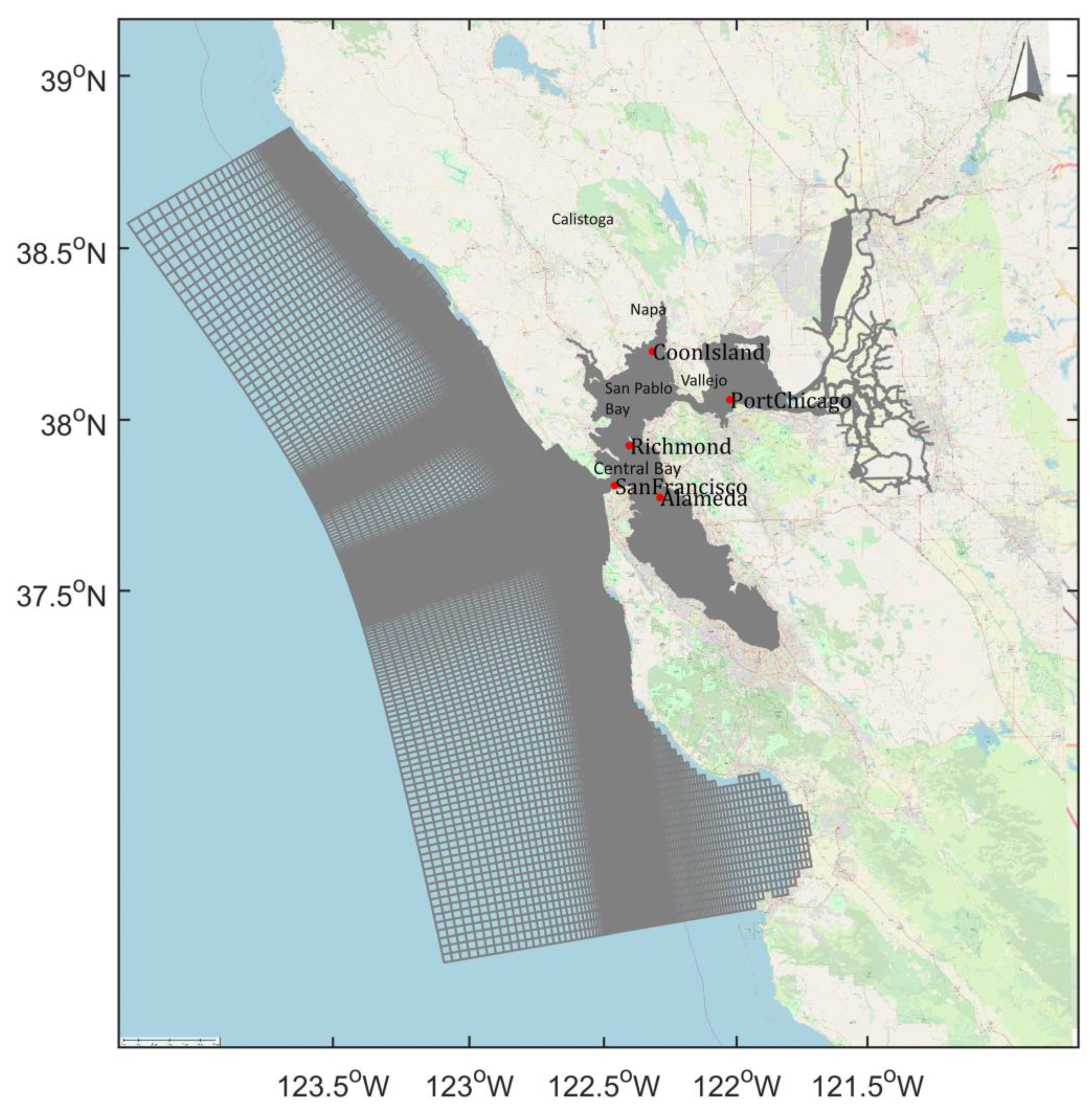
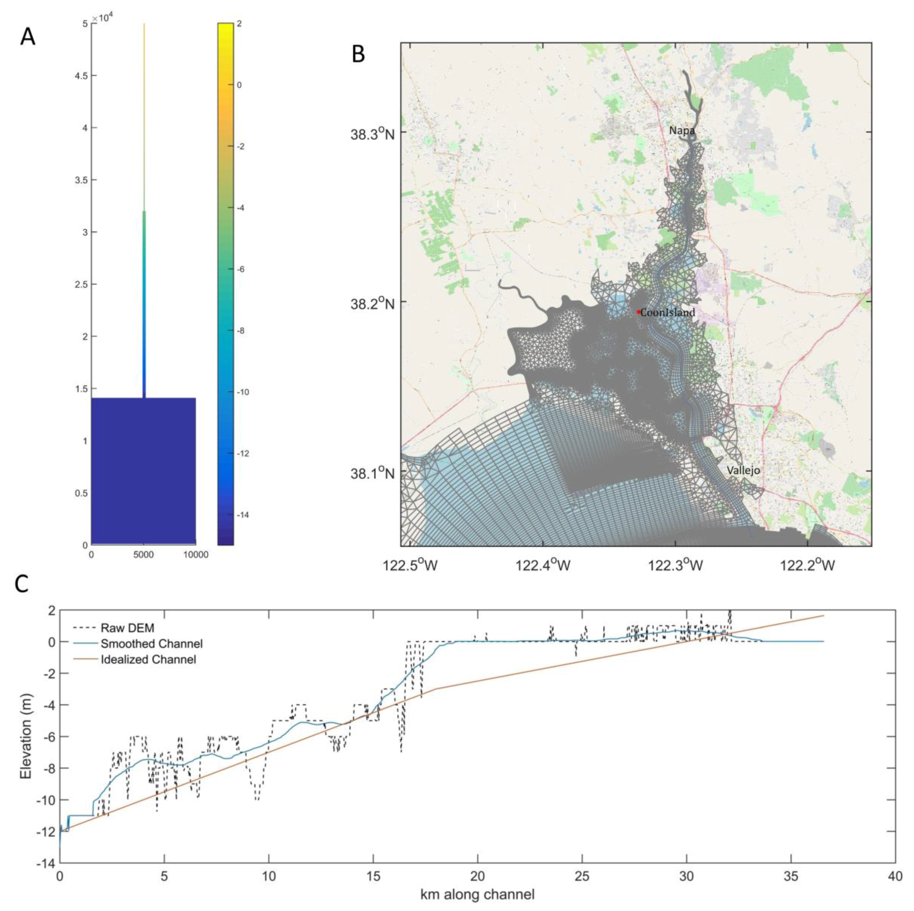
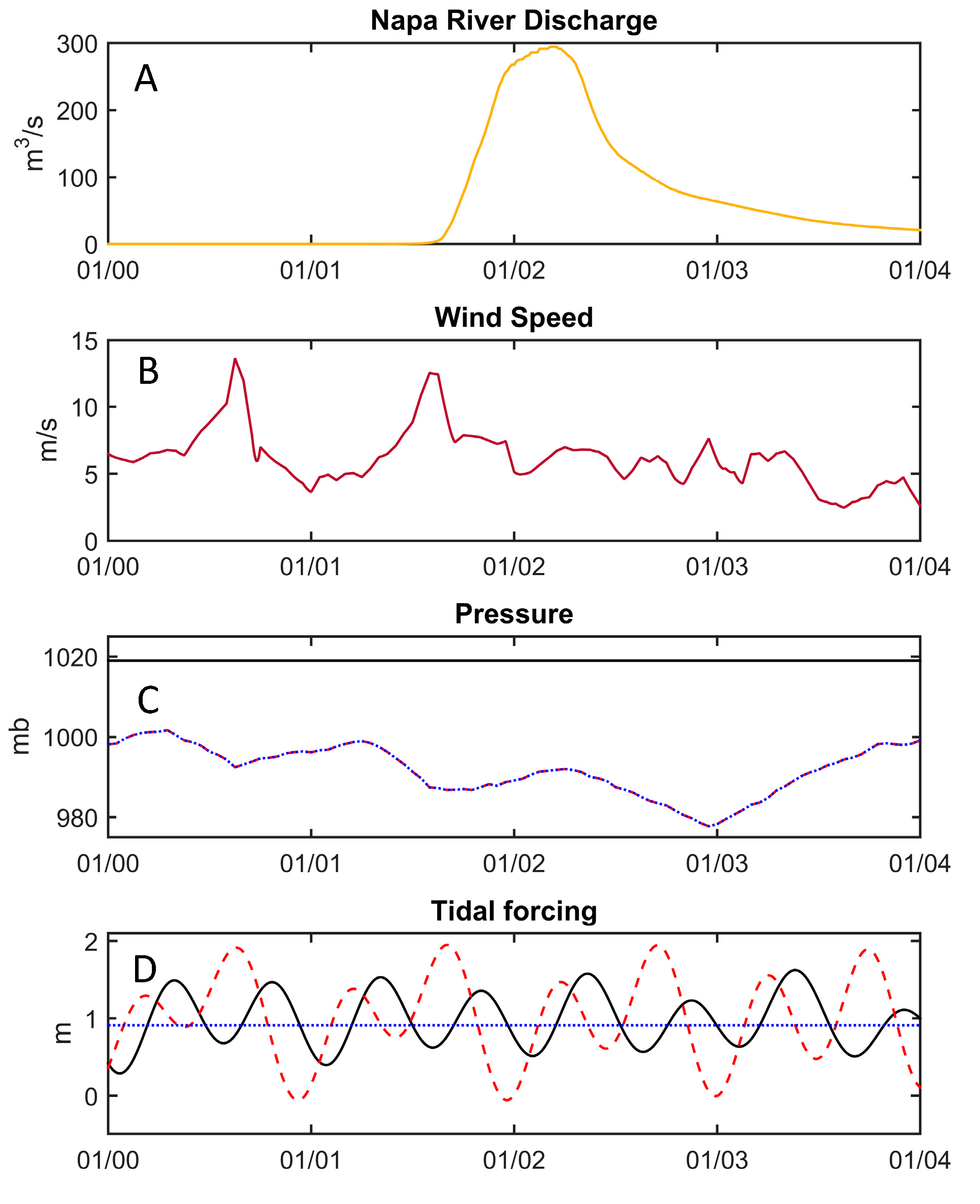
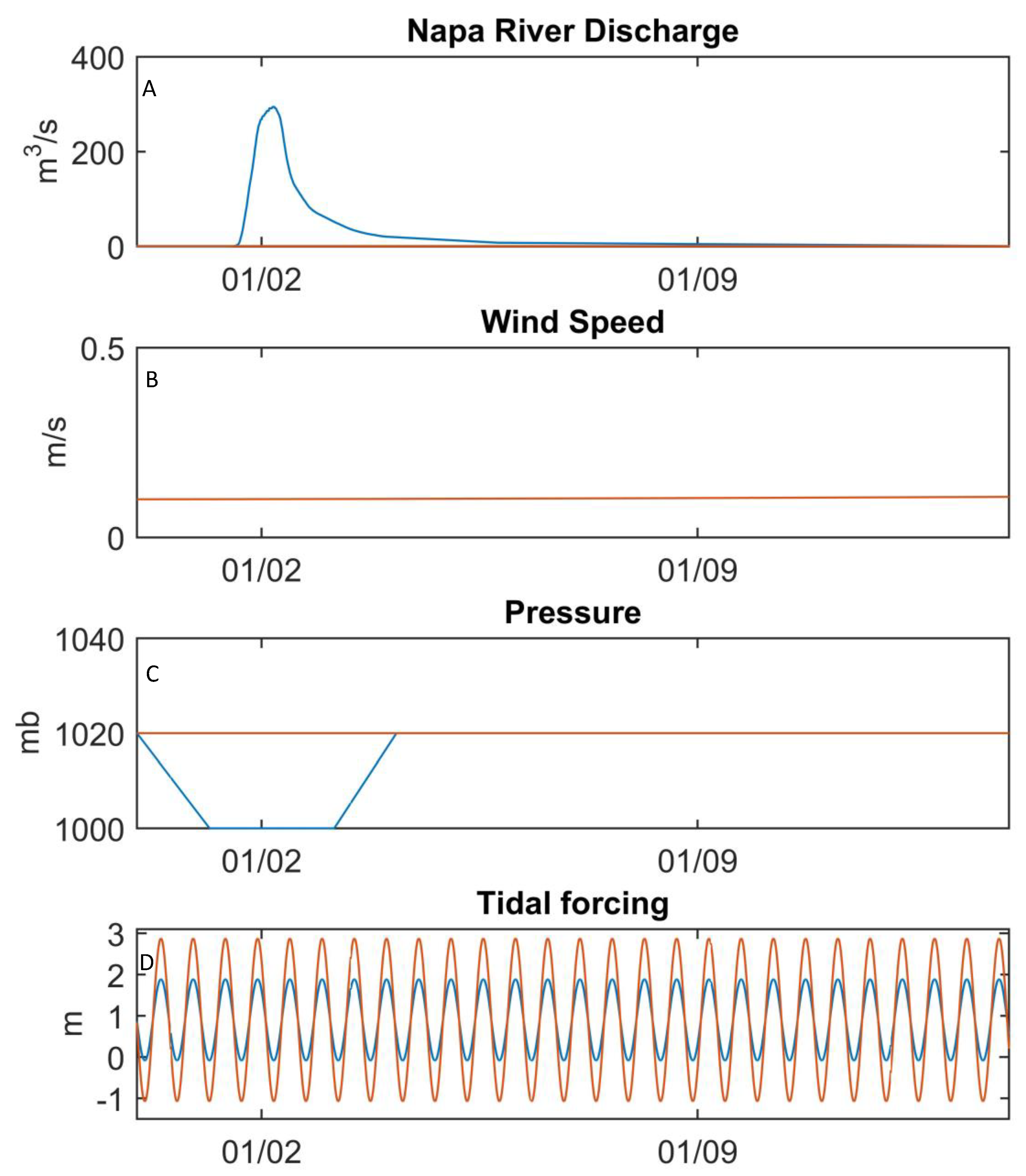
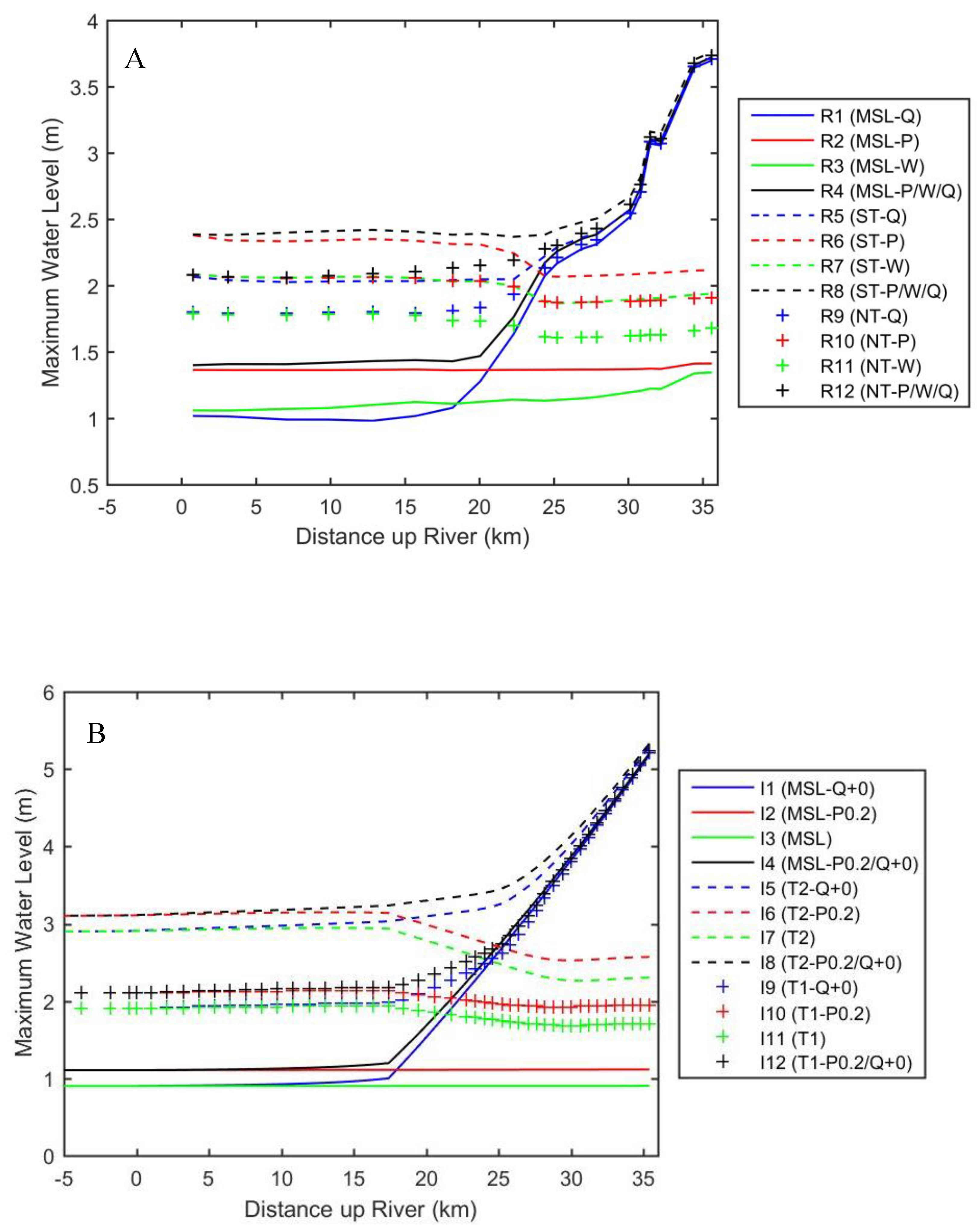
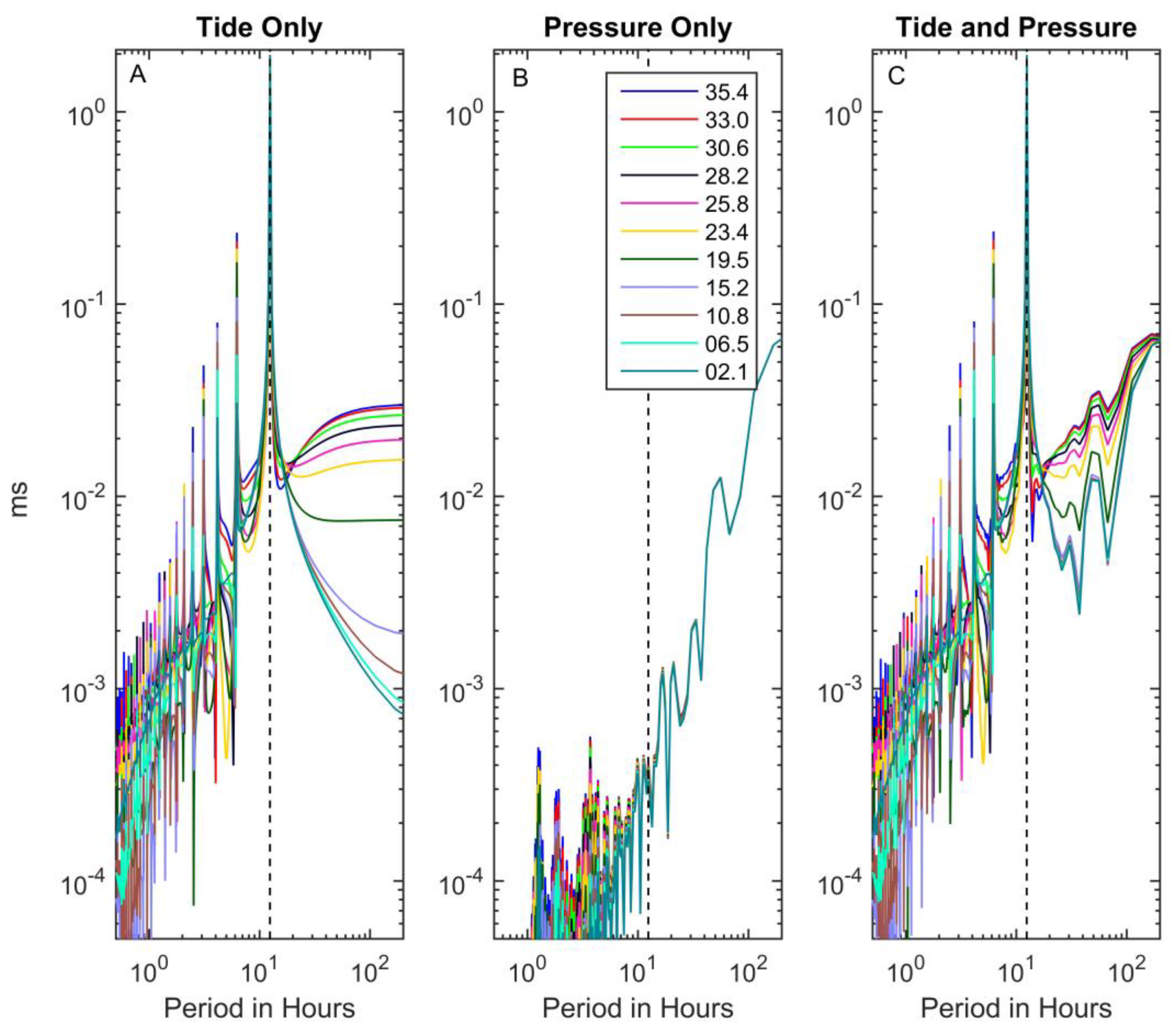
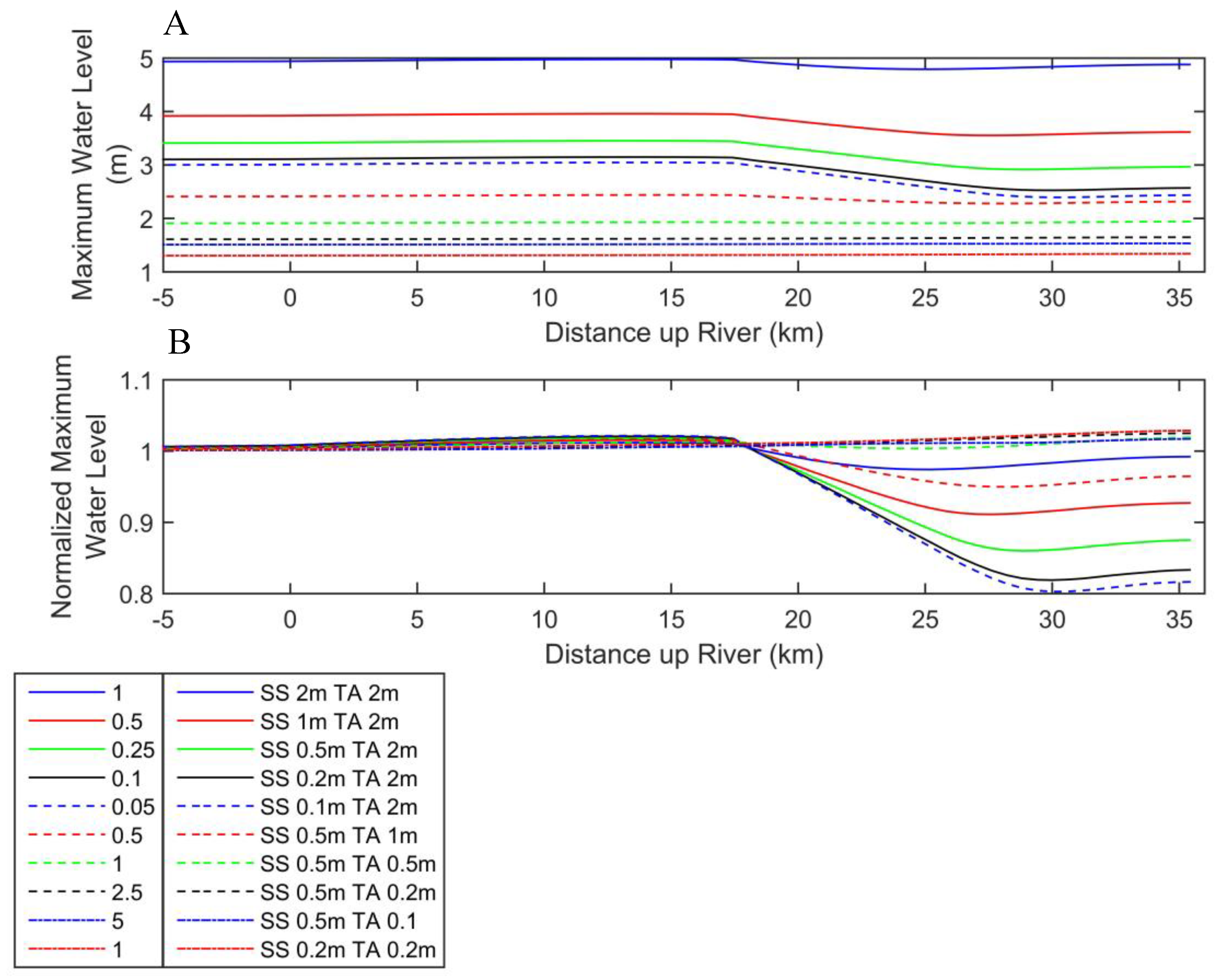
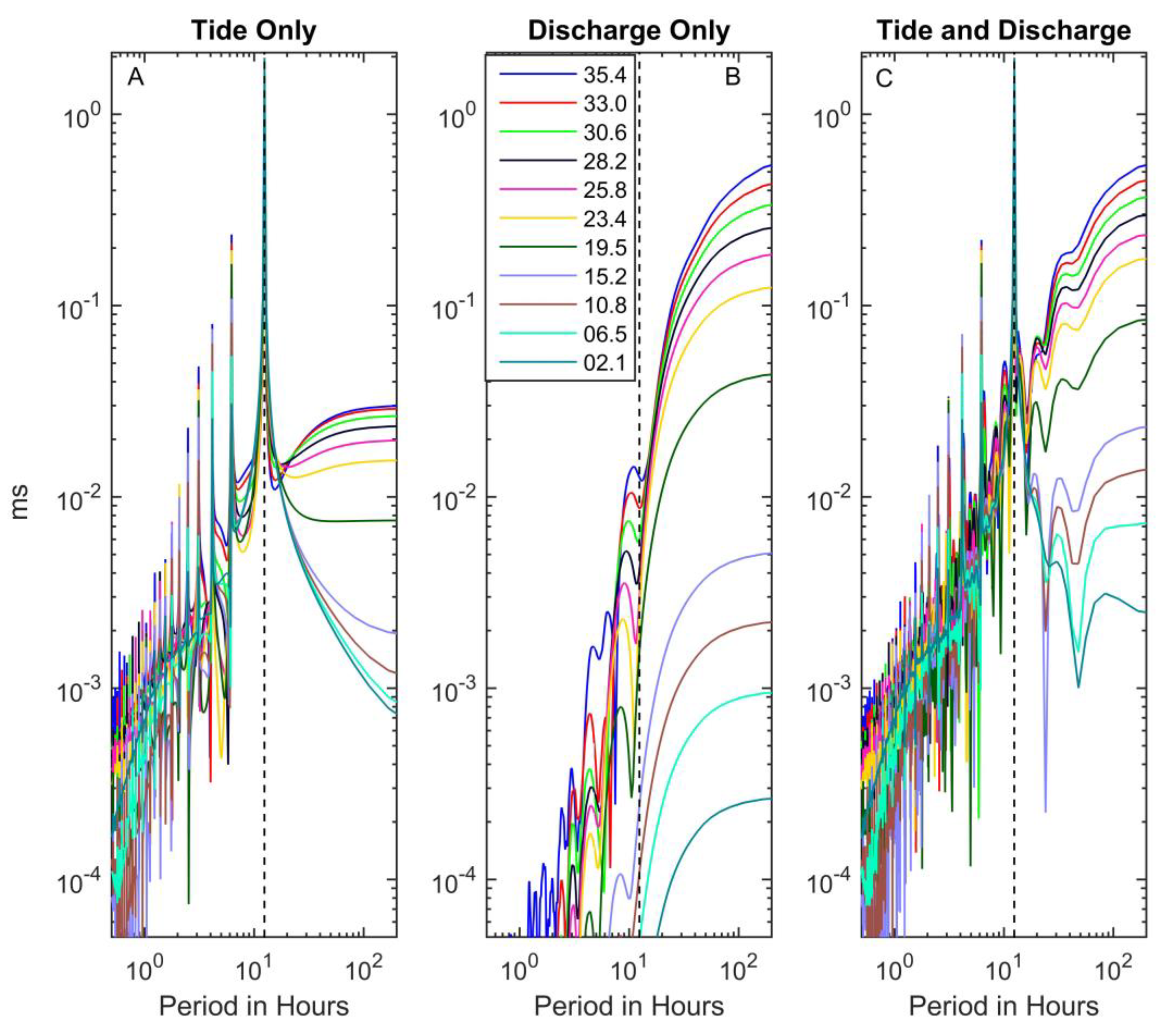
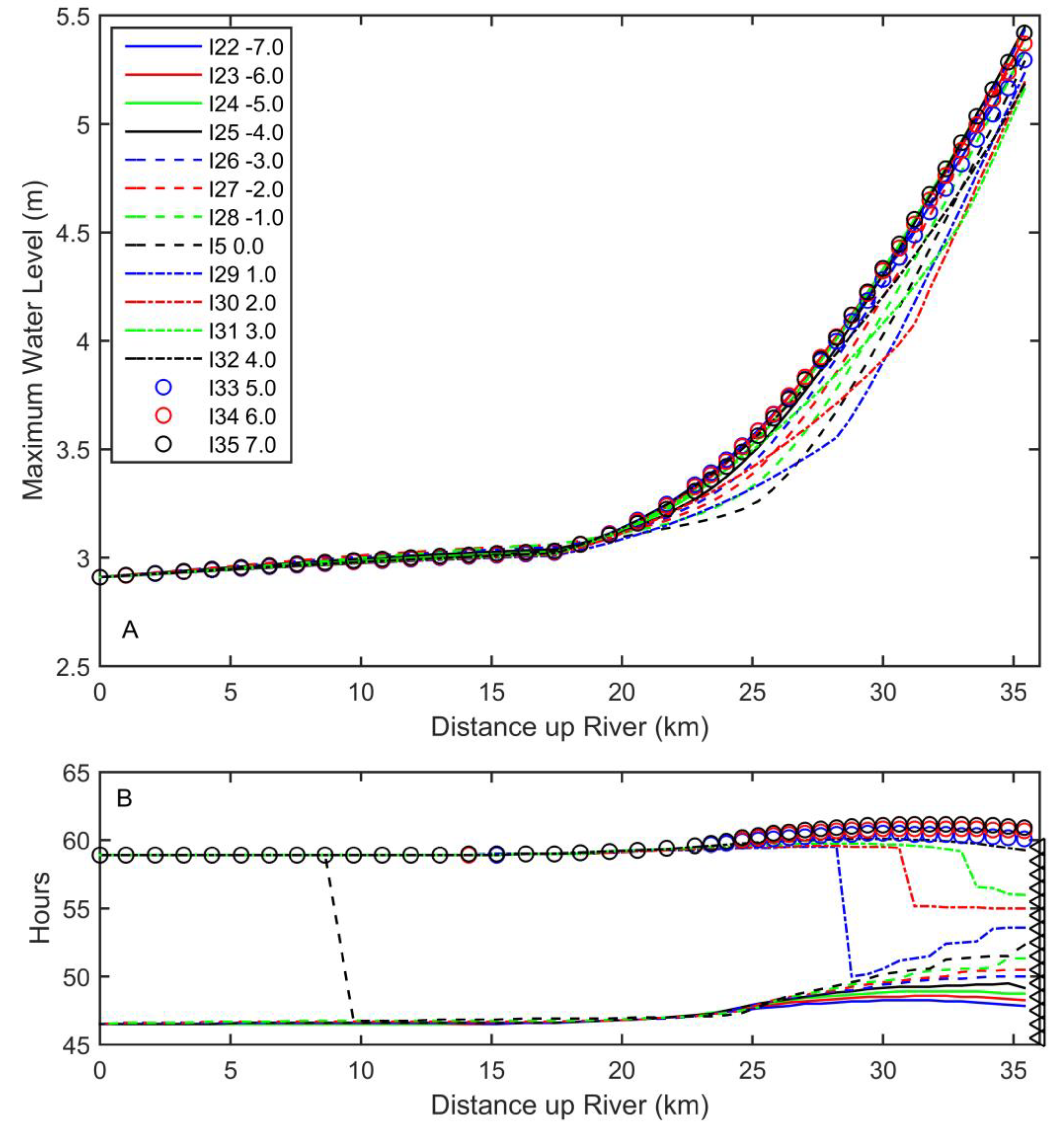
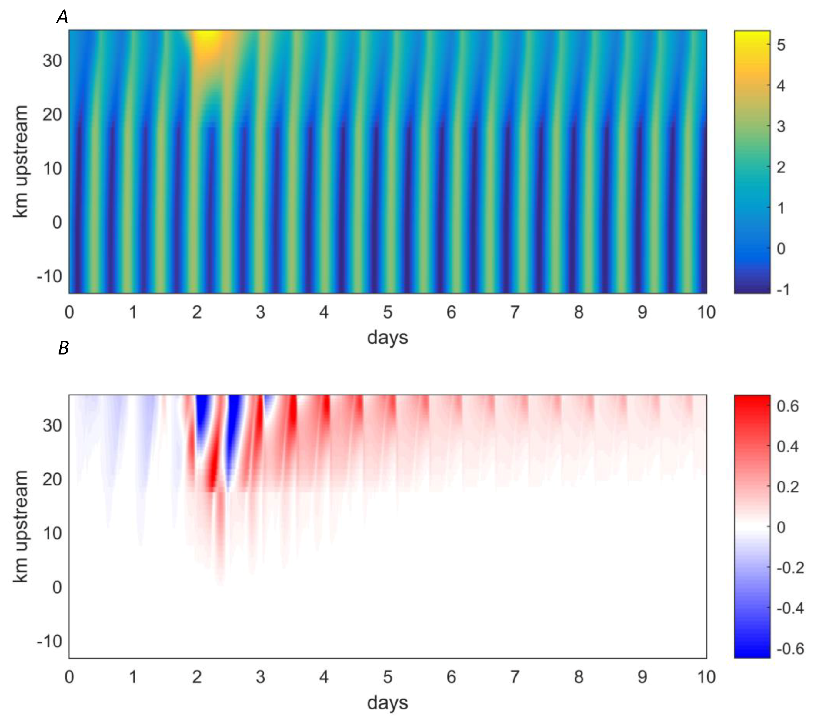
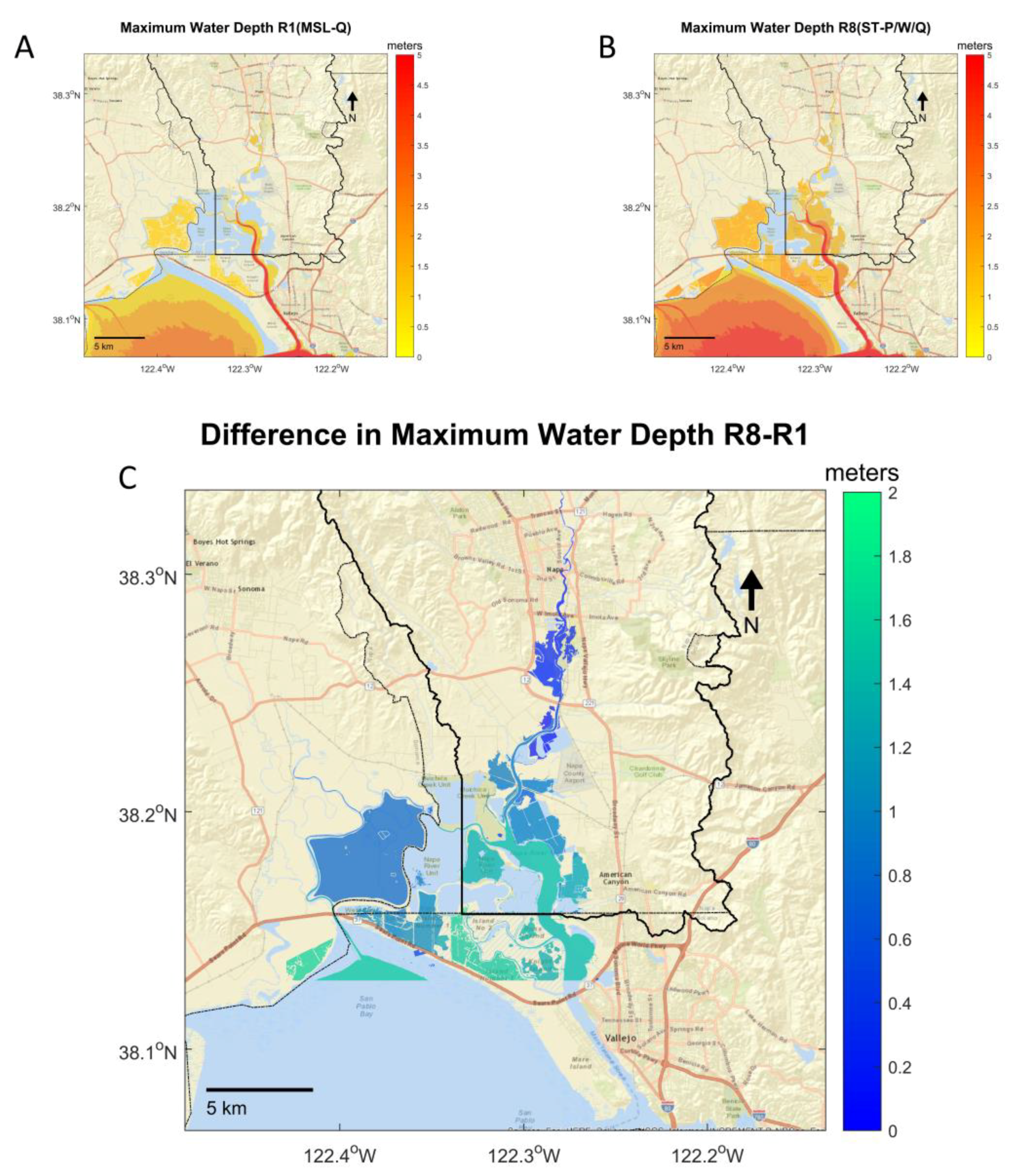
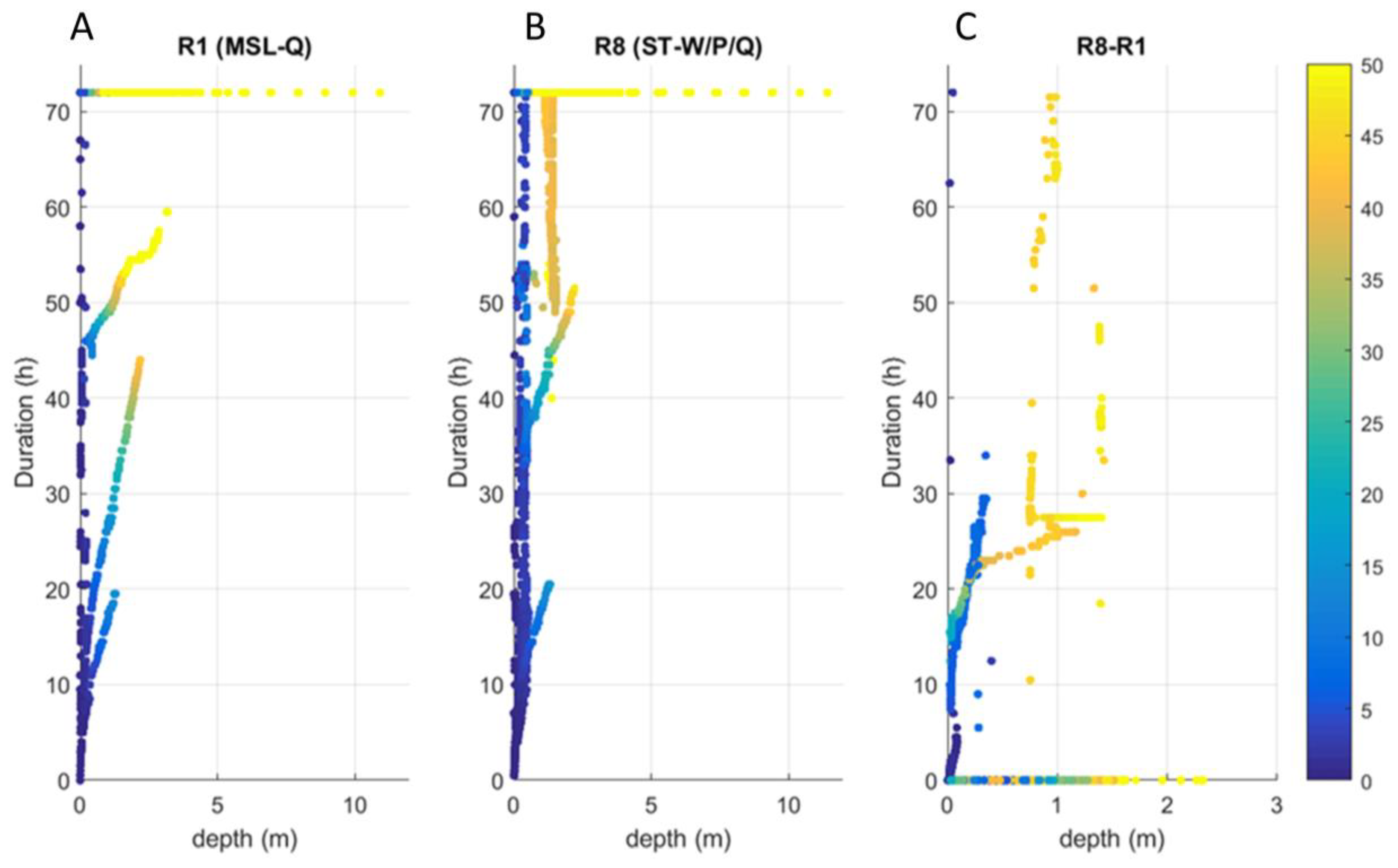
Table 1.
Typical winter river discharges applied to river inlets.
| Freshwater Source | Non-Storm Discharges (m3 s−1) |
|---|---|
| Sacramento River | 500 |
| American River | 45 |
| Arcade Creek | 0.02 |
| Napa River | 5 |
| Petaluma River | 5 |
| Corte Madera Creek | 2 |
| San Joaquin River | 60 |
| San Francisquito Creek | 0.5 |
| Matadero Creek | 0.05 |
| Coyote Creek | 3 |
| Guadalupe River | 2 |
Table 2.
Realistic model scenario titles and forcing included.
| Scenario Name | Water Level | Pressure | Discharge |
|---|---|---|---|
| R1 (MSL-Q) | MSL (Mean Sea Level) Flat | Constant | Storm |
| R2 (MSL-P) | MSL Flat | Storm | Low Normal |
| R3 (MSL-W) | MSL Flat | Constant | Low Normal |
| R4 (MSL-P/W/Q) | MSL Flat | Storm | Storm |
| R5 (ST-Q) | Spring Tide | Constant | Storm |
| R6 (ST-P) | Spring Tide | Storm | Low Normal |
| R7 (ST-W) | Spring Tide | Constant | Low Normal |
| R8 (ST-P//W/Q) | Spring Tide | Storm | Storm |
| R9 (NT-Q) | Neap Tide | Constant | Storm |
| R10 (NT-P) | Neap Tide | Storm | Low Normal |
| R11 (NT, W) | Neap Tide | Constant | Low Normal |
| R12 (NT-P/W/Q) | Neap Tide | Storm | Storm |
Table 3.
Idealized model runs and their forcings.
| Scenario Name | Water Level | Pressure | Discharge |
|---|---|---|---|
| I1 (MSL-Q + 0) | MSL Flat | Constant | Storm |
| I2 (MSL-P0.2) | MSL Flat | 0.2 m Storm | Low Normal |
| I3 (MSL) | MSL Flat | Constant | Low Normal |
| I4 (MSL-P0.2/Q + 0) | MSL Flat | 0.2 m Storm | Storm |
| I5 (T2-Q + 0) | 2 m M2 | Constant | Storm |
| I6 (T2-P0.2) | 2 m M2 | 0.2 m Storm | Low Normal |
| I7 (T2) | 2 m M2 | Constant | Low Normal |
| I8 (T2-P0.2/Q + 0) | 2 m M2 | 0.2 m Storm | Storm |
| I9 (T1-Q + 0) | 1 m M2 | Constant | Storm |
| I10 (T1-P0.2) | 1 m M2 | 0.2 m Storm | Low Normal |
| I11 (T1) | 1 m M2 | Constant | Low Normal |
| I12 (T1-P0.2/Q + 0) | 1 m M2 | 0.2 m Storm | Storm |
| I13 (T2-P2) | 2 m M2 | 2 m Storm | Low Normal |
| I14 (T2-P1) | 2 m M2 | 1 m Storm | Low Normal |
| I15 (T2-P0.5) | 2 m M2 | 0.5 m Storm | Low Normal |
| I16 (T2-P0.1) | 2 m M2 | 0.1 m Storm | Low Normal |
| I17 (T0.2-P0.2) | 0.2 m M2 | 0.2 m Storm | Low Normal |
| I18 (T1-P0.5) | 1 m M2 | 0.5 m Storm | Low Normal |
| I19 (T0.5-P0.5) | 0.5 m M2 | 0.5 m Storm | Low Normal |
| I20 (T0.2-P0.5) | 0.2 m M2 | 0.5 m Storm | Low Normal |
| I21 (T0.1-P0.5) | 0.1 m M2 | 0.5 m Storm | Low Normal |
| I22 (T2-Q − 7) | 2 m M2 | Constant | Storm − 7 h |
| I23 (T2-Q − 6) | 2 m M2 | Constant | Storm − 6 h |
| I24 (T2-Q − 5) | 2 m M2 | Constant | Storm − 5 h |
| I25 (T2-Q − 4) | 2 m M2 | Constant | Storm − 4 h |
| I26 (T2-Q − 3) | 2 m M2 | Constant | Storm − 3 h |
| I27 (T2-Q − 2) | 2 m M2 | Constant | Storm – 2 h |
| I28 (T2-Q − 1) | 2 m M2 | Constant | Storm − 1 h |
| I29 (T2-Q + 1) | 2 m M2 | Constant | Storm + 1 h |
| I30 (T2-Q + 2) | 2 m M2 | Constant | Storm + 2 h |
| I31 (T2-Q + 3) | 2 m M2 | Constant | Storm + 3 h |
| I32 (T2-Q + 4) | 2 m M2 | Constant | Storm + 4 h |
| I33 (T2-Q + 5) | 2 m M2 | Constant | Storm + 5 h |
| I34 (T2-Q + 6) | 2 m M2 | Constant | Storm + 6 h |
| I35 (T2-Q + 7) | 2 m M2 | Constant | Storm + 7 h |
Table 4.
Skill statistics comparing modeled and observed water levels.
| Station | Observed Diurnal Range (m) | Mean Error (m) | Wilmott Skill Score (D) | Coeff. of Efficiency (E) | |||
|---|---|---|---|---|---|---|---|
| January 2010 | March 2011 | January 2010 | March 2011 | January 2010 | March 2011 | ||
| San Francisco | 1.78 | −0.04 | −0.01 | 0.99 | 0.99 | 0.74 | 0.44 |
| Richmond | 1.85 | −0.01 | −0.05 | 0.99 | 0.98 | 0.73 | 0.43 |
| Port Chicago | 1.50 | −0.05 | −0.11 | 0.97 | 0.96 | 0.51 | 0.38 |
| Coon Island | NA | NA | −0.15 | NA | 0.87 | NA | 0.72 |
© 2018 by the authors. Licensee MDPI, Basel, Switzerland. This article is an open access article distributed under the terms and conditions of the Creative Commons Attribution (CC BY) license (http://creativecommons.org/licenses/by/4.0/).
Share and Cite
MDPI and ACS Style
Herdman, L.; Erikson, L.; Barnard, P. Storm Surge Propagation and Flooding in Small Tidal Rivers during Events of Mixed Coastal and Fluvial Influence. J. Mar. Sci. Eng. 2018, 6, 158. https://doi.org/10.3390/jmse6040158
AMA Style
Herdman L, Erikson L, Barnard P. Storm Surge Propagation and Flooding in Small Tidal Rivers during Events of Mixed Coastal and Fluvial Influence. Journal of Marine Science and Engineering. 2018; 6(4):158. https://doi.org/10.3390/jmse6040158
Chicago/Turabian StyleHerdman, Liv, Li Erikson, and Patrick Barnard. 2018. "Storm Surge Propagation and Flooding in Small Tidal Rivers during Events of Mixed Coastal and Fluvial Influence" Journal of Marine Science and Engineering 6, no. 4: 158. https://doi.org/10.3390/jmse6040158
Note that from the first issue of 2016, this journal uses article numbers instead of page numbers. See further details here.