Integrating Multiple-Try DREAM_(ZS) to Model-Based Bayesian Geoacoustic Inversion Applied to Seabed Backscattering Strength Measurements

Abstract

The key to model-based Bayesian geoacoustic inversion is to solve the posterior probability distributions (PPDs) of parameters. In order to obtain PPDs more efficiently and accurately, the state-of-the-art Markov chain Monte Carlo (MCMC) method, multiple-try differential evolution adaptive Metropolis_(ZS) (MT-DREAM_(ZS)), is integrated to the inverse problem because of its excellent ability to fully explore the posterior space of parameters. The effective density fluid model (EDFM), which is derived from Biot–Stoll theory to approximate the poroelastic model, and the published field measurements of backscattering strength are adopted to implement the inversion. The results show that part of the parameters can be estimated close to the measured values, and the PPDs obtained by dual-frequency inversion are more concentrated than those of single-frequency inversion because of the use of more measured backscattering strength data. Otherwise, the comparison between the predicted backscattering strength of dual-frequency inversion results and Jackson’s prediction shows that the solutions of the inverse problem are not unique and may have multiple optimal values. Indeed, the difference between the two predictions is essentially the difference in the estimation of the contribution of volume scattering to the total scattering. Nevertheless, both results are reasonable due to the lack of measurement of volume scattering parameters, and the inversion results given by the posterior probabilities based on the limited measurements and the adopted model are still considered to be reliable.

1. Introduction

In the field of oceanography, high-frequency underwater sound is widely used in active sonar to detect underwater targets such as submarines, mines, underwater structures, and animals with a relatively adequate resolution [1,2]. In this case, acoustic scattering from the seafloor becomes a disturbance to the target signal, and that leads us to try to understand which kinds of acoustic interference would be caused by different types of sediments. On the other hand, for applications such as marine geology, marine biology, and coastal engineering, the sediment is the target, and the acoustic interference becomes the target signal which can be used to obtain the detailed information about sediment. In either case, it can be found that understanding the interaction between sound waves and sediment is very important for the application of active sonar systems and the detection of sediment [3,4,5]. This motivates the modeling of acoustic scattering at the water–seabed interface and deeper sediment layers [6,7].

Seabed acoustic modelers are trying to solve a forward problem. Predicted data are calculated by ${\mathit{d}}^{pre}=f\left(\mathit{m}\right)$, where the function $f$ represents the physical process of sound waves and $\mathit{m}$ is a set of measured model parameters. The predicted data ${\mathit{d}}^{pre}$ are then compared with the observed data ${\mathit{d}}^{obs}$ to verify or correct the model. For seabed scattering, although it is artificial to divide this into interface scattering and volume scattering, this distinguishing method has still been taken as a mathematical approximation and fitting between measurements and model predictions. The earlier and simpler model of seabed scattering—the fluid model, which takes the sediment as a fluid layer—has applied this distinguishing method [8]. The comparison between the fluid model prediction and measurements has been completed and has been shown to be successful to some extent [9,10]. As a porous medium, sandy sediment is prevalent in coastal environments, and it may be more reasonable to model sandy sediment by the poroelastic model than the fluid model. The earlier poroelastic model was derived from Biot theory and used to model acoustic scattering by Stoll [11]. Then, the Born approximation (first-order perturbation theory) of a fluid model was extended to the poroelastic model based on the Biot–Stoll theory [12]. The comparison of the model predictions between the fluid and poroelastic models indicated that the predicted backscattering levels of the poroelastic model for sandy sediments are substantially lower than those of the fluid model and more consistent with the measurements [13]. In order to further reduce the mismatch between poroelastic model prediction and measurements, the physics of grain–grain contact and multiple scattering losses were added, and the input parameters were adjusted to increase the efficiency of simulating multiple sediment types [14]. Although such poroelastic models have inherent advantages over the fluid model for sandy sediment, they suffer from more computational cost. To solve this problem, an EDFM derived from Biot–Stoll theory was used to model acoustic scattering at the seabed–water interface [15]. This model utilizes a bulk modulus and an effective density derived from Biot–Stoll theory in the fluid model to obtain predictions including dispersion, transmission, reflection, and scattering, which are very close to those of the poroelastic model for sandy sediment [13,16,17]. As the fluid model does not include grain–grain contact by fiat, additional acoustic dispersion and attenuation are added to EDFM though additional physical mechanisms, which are the transfer of heat between the liquid and solid at low frequencies and the effect of granularity at high frequencies [18].

Geoacoustic inversion workers aim to solve an inverse problem. When a validated model function $f$ with a set of observations ${\mathit{d}}^{obs}$ is obtained, the vector of the model parameters $\mathit{m}$ can be estimated by $\widehat{m}=f^{-1}\left({\mathit{d}}^{obs}\right)$. However, for the nonlinear model of acoustic scattering from the seabed, an analytic form of $f^{-1}$ rarely exists. An iterative search and global optimization algorithm are naturally applied to model-based geoacoustic inversion, and a point estimate of parameters can be obtained [5,19]. By contrast, Bayesian inference is perfectly applicable to an inverse problem as it can rigorously provide nonlinear quantitative uncertainty distributions of parameters which are treated as random variables instead of point estimates [20,21,22,23]. The key task in model-based Bayesian geoacoustic inversion is to solve the PPDs, and the basic idea is to use MCMC methods. A random walk within the Markov chain can explore the posterior space and iteratively find a relatively stable probability distribution, which is an approximate estimate of the target posterior probability distribution [24,25,26,27]. When faced with a PPD which has higher parameter dimensions and a more complex posterior distribution, the original MCMC methods such as the well-known random walk Metropolis (RWM) algorithm [28] and the Metropolis-Hastings algorithm (MH) [24] may suffer from low convergence efficiency because of the selection of the proposal distribution. To solve this problem, the idea of self-adaptive proposal is adopted in MCMC methods such as the adaptive Metropolis (AM) [25] and the delayed rejection adaptive Metropolis (DRAM) [27] algorithms. However, these MCMC methods are essentially single-chain, and this motivates a major improvement in that multiple chains running in parallel are adopted to explore the target posterior distribution. This improvement allows the MCMC methods to handle more complex posterior distributions and avoid premature convergence. Representative multi-chain MCMC methods include the shuffled complex evolution Metropolis (SCEM) [29] and differential evolution Markov chain (DE-MC) [30]. Vrugt and coworkers further enhanced the efficiency of DE-MC using self-adaptive randomized subspace sampling and the explicit consideration of aberrant trajectories. Then, a series of differential evolution adaptive Metropolis (DREAM) algorithms was proposed [31,32]. As the most advanced one within the series of algorithms proposed by Vrugt and coworkers, MT-DREAM_(ZS) combines the strengths of differential evolution, subspace exploration, sampling from past states, snooker updating, and multiple-try Metropolis sampling and can achieve the more efficient exploration of the parameter posterior space of highly parameterized models [33].

Indeed, MCMC methods have already been applied to Bayesian geoacoustic inversion. Dosso has successfully applied a single-chain MCMC method to quantify uncertainty in geoacoustic inversion [20,34,35]. Bonomo utilized the Metropolis–Hastings algorithm to explore the parameter posterior space and compared several models [36]. However, Bonomo also pointed out that low likelihood regions in the parameter space may not be fully explored using the Metropolis–Hastings algorithm. Most geoacoustic inversion workers do not focus on the method of solving PPDs, although this is a crucial step and has a great impact on the inversion efficiency and results. Therefore, it is necessary to introduce a more efficient and accurate method for solving PPD into Bayesian inversion. Although the original DREAM methods have been successfully applied to geoacoustic inversion to evaluate the main scattering mechanism and select the model that best matches the measurements [37,38], the inversion results based on DREAM have not been verified by field measurements.

The aim of this paper is to integrate the state-of-the-art MCMC method—MT-DREAM_(ZS)—to model-based Bayesian geoacoustic inversion. EDFM is used as the inversion model due to its relatively small computational cost and a model prediction that is close to the poroelastic model. Published field backscattering strength data at the Quinault site [8] are used here to implement geoacoustic inversion, and the inversion results can be compared with the measured sediment properties. The authors believe that this is the first time that MT-DREAM_(ZS) is applied to model-based Bayesian geoacoustic inversion using field measurements. Although this method was originally applied to the field of hydrology [33], the intent of the method developers is to apply it to complex system models with observations for the purpose of learning and scientific discovery, enhancing the growth of environmental knowledge. In this paper, the environmental knowledge includes the characteristics of seabed sediment, and the remainder of this paper is organized as follows: An introduction of the EDFM and a brief review of model-based Bayesian geoacoustic inversion and MT-DREAM_(ZS) methods are given in Section 2. The field experiments at the Quinault site, parameter inversion results, and comparison with measurements are presented in Section 3. Finally, this work is concluded in Section 4.

2. Methodology

Model-based Bayesian geoacoustic inversion is the process of obtaining parameters of sediment properties by Bayesian inversion based on a particular geoacoustic model and measured model outputs. In an inverse problem, the focus is not on the validity of the model, which is the topic of the forward problem. That is, when a model is selected for inversion, it is accepted that the model may have a limited validity, and the purpose of inversion is to give the best answer based on the selected model and measurements. In this paper, a validated model with moderate computational cost is selected for inversion. In order to give the inversion results with rigorously quantitative uncertainty, Bayesian inversion is adopted. MT-DREAM_(ZS) is selected and applied to geoacoustic inversion due to its proven efficiency and accuracy for estimating PPDs. Below, we will briefly explain the content of these aspects.

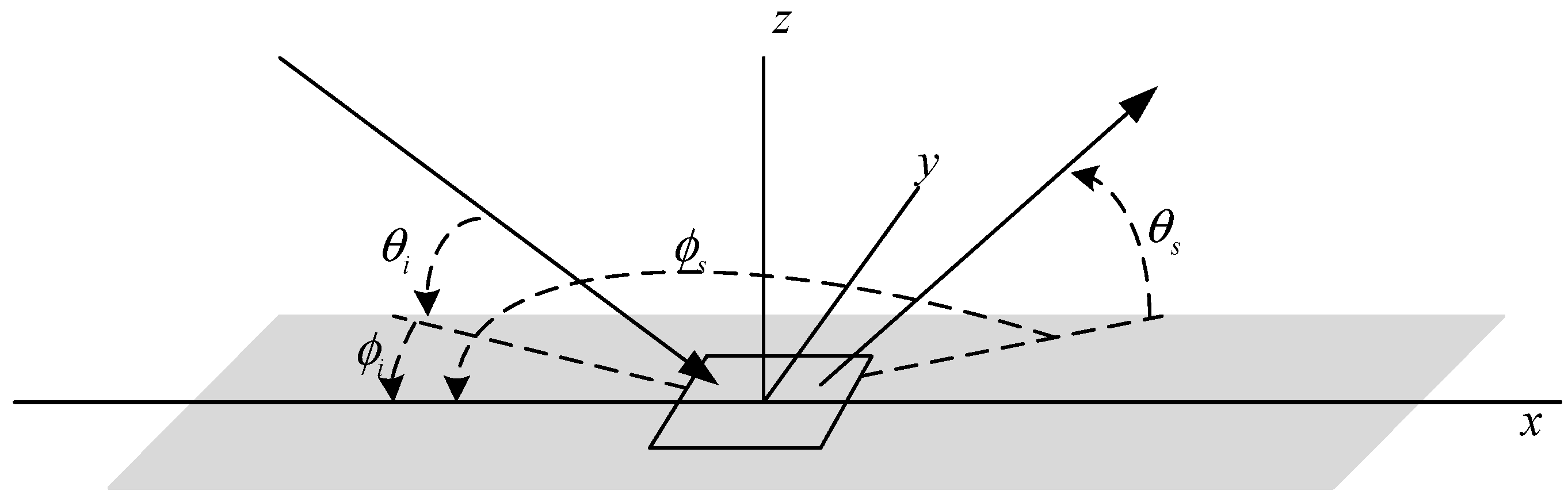
2.1. Acoustic Scattering Model Based on Effective Density Fluid Approximation

EDFM is an effective density fluid approximation for the poroelastic model based on the full Biot–Stoll theory. The essence of the approximation is to start by setting the two relatively small frame moduli in Biot–Stoll theory to zero. Then, the effective density can be derived from the equations of motion. The final scattering strength can be obtained through the fluid interface scattering model and volume scattering model through the simple parameter replacement of density by effective density. The specific approximate derivation process can be found in [15], and below, we give the main calculation process of scattering strength.

The fluid model requires seven input parameters: The roughness spectral exponent ${\gamma }_2$, roughness spectral strength ${\omega }_2$, density fluctuation spectral exponent ${\gamma }_3$, density fluctuation spectral strength ${\omega }_3$, ratio of compressibility to density fluctuation in sediment $\mu$, density ratio $a_{\rho }$, and complex velocity ratio $a_1$. The scattering strength $S_b$ can be obtained by [39]

$$S_b=10{\log }_{10}({\sigma }_{bI}+{\sigma }_{bV})$$

(1)

$${\sigma }_{bI}=(k_w^4{|[1+V_{ww}({\theta }_i)][1+V_{ww}({\theta }_s)]G|}^2{I}_k)∕(8\pi \mathsf{\Delta }{K}^2\mathsf{\Delta }{k}_z^2)$$

(2)

$${\sigma }_{bV}=\frac{{\left|1+V_{ww}\left({\theta }_i\right)\right|}^2{\left|1+V_{ww}\left({\theta }_s\right)\right|}^2{\sigma }_v}{2k_w{\left|a_{\rho }\right|}^2\mathrm{Im}\left(\sqrt{1/a_1^2-{\cos }^2{\theta }_i}+\sqrt{1/a_1^2-{\cos }^2{\theta }_s}\right)}$$

(3)

where ${\sigma }_{bI}$ represents the rough scattering cross-section using small-slope approximation, ${\sigma }_{bV}$ represents the volume scattering cross-section, and $k_w$ is the acoustic wavenumber in water. The flat-interface reflection coefficient $V_{ww}$, factor $G$, and Kirchhoff integrals $I_k$, $\mathsf{\Delta }K$, $\mathsf{\Delta }{k}_z$ which, respectively, denote the magnitude of the horizontal and vertical vector difference between the scattered wave and the incident wave, are given in the Appendix. The expression of ${\sigma }_{bV}$ is the basis of several sediment volume scattering models, which differ only in the assumptions used to obtain the factor ${\sigma }_v$. Indeed, the inhomogeneities within the sediment are so difficult to measure that Jackson had to take the sediment volume scattering parameter as a free parameter [8]. As the simplest approach, ${\sigma }_v$ can be obtained by a data fitting parameter ${\sigma }_2$ empirically [40]:

$${\sigma }_v={\sigma }_2{\alpha }_p$$

(4)

where ${\alpha }_p$ is the attenuation in dB/m, and ${\sigma }_2$ is a dimensionless parameter used as a fitting adjustment parameter. In contrast, the theory-based ${\sigma }_v$ is adopted in the inversion of this paper and can be obtained using the small-perturbation fluid approximation in [10,41]:

$${\sigma }_v=\frac{\pi }{2}{k}_w^4{\left|\mu ∕a_1^2+\cos {\theta }_i\cos {\theta }_s\cos {\varnothing }_s-\sqrt{1/a_1^2-{\cos }^2{\theta }_i}\sqrt{1/a_1^2-{\cos }^2{\theta }_s}\right|}^2\frac{w_3}{{\left(\mathsf{\Delta }{k}_p\right)}^{{\gamma }_3}}$$

(5)

where $\mathsf{\Delta }{k}_p$ is the real part of the vector difference of the scattered and incident waves that propagate in sediment and is given in the Appendix. Definitions of all angles ${\theta }_i$, ${\theta }_s$, ${\varnothing }_s$ are also in the Appendix. By the comparison of Equations (4) and (5), it can be seen that the empirical ${\sigma }_v$ is fixed while the theoretical ${\sigma }_v$ varies with the angle if the frequency is fixed.

The above is a brief calculation process of the fluid scattering model. The following is the calculation process of the density ratio $a_{\rho }$ and complex velocity ratio $a_1$ derived from Biot–Stoll theory. Ten input parameters are required: The mean grain diameter $d$, tortuosity $\alpha$, porosity $\beta$, dynamic viscosity of water $\eta$, permeability $\kappa$, mass density of water ${\rho }_w$, mass density of grains ${\rho }_g$, bulk modulus of water $K_w$, bulk modulus of grains $K_g$, and compressional wave speed in water $c_w$. As the inversion in this paper is based on the measurements at high frequencies, the improved EDFM with the effect of granularity is given here. The density ratio $a_{\rho }$ and complex velocity ratio $a_1$ can be obtained by [15,18]

$$a_{\rho }={\rho }_{eff}/{\rho }_w$$

(6)

$$a_1=\sqrt{{\xi }_{\mathrm{DM}}\left(\lambda ,d;\theta =30°\right){\left[\left(1-\beta \right)/K_g+\beta /K_w\right]}^{-1}/{\rho }_{eff}}/c_w$$

(7)

where $\lambda =c_w∕f$ is the wavelength of a sound wave in water. The effective density ${\rho }_{eff}$ and granularity effect correction factor ${\xi }_{\mathrm{DM}}$ are given in the Appendix. The compressional velocity ratio can be obtained by

$$v_1=\frac{1}{c_w}/\mathrm{Re}\left(1/a_1/c_w\right)$$

(8)

Since the effect of granularity does not have enough physics to account for additional multiple scattering loss, the effect is added to the attenuation calculated via the imaginary part of the sound speed equation using the following expression [42]:

$${\mathsf{\alpha }}_{ms}=24{\left(2\pi fd∕c_w\right)}^4$$

(9)

The final attenuation is expressed as

$${\alpha }_p=40\pi fIm\left(1/a_1/c_w\right)/ln\left(10\right)+{\mathsf{\alpha }}_{ms}$$

(10)

It needs to be noted here that the unit of attenuation is dB/m. Then, the final modified complex velocity ratio ${\mathrm{a}}_1$ can be obtained by

$$a_1={\left[1/v_1/c_w+i{\alpha }_{p}ln\left(10\right)∕\left(40\pi f\right)\right]}^{-1}$$

(11)

By substituting the density ratio $a_{\rho }$ and complex velocity ratio $a_1$ into the original fluid scattering model, the fluid model is extended to poroelastic media.

2.2. Model-Based Bayesian Inversion

When estimates of model inputs are obtained based on model and measured outputs, there may be multiple optimal estimates. The global optimization algorithm is an intuitive solution to this problem, although repeated runs may yield different answers. Indeed, it is not rigorous to provide an answer with only one or a set of point estimates. Bayesian inversion is the most appropriate and rigorous way to solve such problems as it considers the model input parameters as random variables and can give quantitative uncertainties. This solution is truly complete from a mathematical point of view. Bayesian inversion has been widely applied to various geoacoustic model inversions and more complete treatments of Bayesian inversion can be found elsewhere [43,44,45,46,47]. Only a brief description is given here, and the original Bayesian formula is

$$P\left(\mathit{m}|\mathit{d}\right)P\left(\mathit{d}\right)=P\left(\mathit{d}|\mathit{m}\right)P\left(\mathit{m}\right)$$

(12)

In an inverse problem, we can take $\mathit{m}$ as the model input parameter vector and $\mathit{d}$ as the vector of measurements. Then, $P\left(\mathit{m}|\mathit{d}\right)$ represents the PPD of $\mathit{m}$ based on the model and is the complete solution of the inverse problem. $P\left(\mathit{d}|\mathit{m}\right)$ denotes the conditional probability distribution of measurements and is interpreted as a likelihood function in Bayesian inversion. $P\left(\mathit{d}\right)$ is independent of $\mathit{m}$ and can be regarded as equal to one. $P\left(\mathit{m}\right)$ represents the prior distribution of $\mathit{m}$. Then, the PPD can be rewritten as

$$P\left(\mathit{m}|{\mathit{d}}^{obs}\right)\propto P\left({\mathit{d}}^{obs}|\mathit{m}\right)P\left(\mathit{m}\right)=L\left(\mathit{m}\right)P\left(\mathit{m}\right)$$

(13)

where $L\left(\mathit{m}\right)\propto \exp \left[-E\left(\mathit{m}\right)\right]$ and $E\left(\mathit{m}\right)$ is the misfit function. For assumed Gaussian errors, $E\left(\mathit{m}\right)$ can be expressed as

$$E\left(\mathit{m}\right)=\left({\mathit{d}}^{obs}-{\mathit{d}}^{pre}\right)\ast {\mathit{C}}_d^{-1}\left({\mathit{d}}^{obs}-{\mathit{d}}^{pre}\right)$$

(14)

where ${\mathit{C}}_d$ is the data error covariance matrix and $\ast$ represents the conjugate transposition. Indeed, the error of observations, which consists of the measurement error and model error, are difficult to specify. Nevertheless, the errors of measurements can be estimated simultaneously with the model inputs within the inversion process, and this is a simple and effective method. Assuming the measurement errors are independent Gaussian-distributed random processes, then the covariance matrix ${\mathit{C}}_d$ and the likelihood function can be expressed as

$${\mathit{C}}_d=\mathrm{diag}\left({\sigma }_1,{\sigma }_2,\dots ,{\sigma }_{N_{\mathrm{d}}}\right)$$

(15)

$$L\left(\mathit{m}\right)=\frac{1}{{\left(2\pi \right)}^{N_d/2}{{\displaystyle \prod }}_{i=1}^{N_d}{\sigma }_i}\exp \left[-\frac{1}{2}{\displaystyle \sum }_{i=1}^{N_d}\frac{{\left(d_i^{obs}-d_i^{pre}\right)}^2}{{\sigma }_i^2}\right]$$

(16)

where $N_{\mathrm{d}}$ is the dimension of ${\mathit{d}}^{obs}$, $d_i^{obs}$ and $d_i^{pre}$ represent the ith element of ${\mathit{d}}^{obs}$ and ${\mathit{d}}^{pre},$ respectively, and ${\sigma }_i,i=1,\dots ,N_{\mathrm{d}}$ is the standard deviation for $d_i^{obs}$. The $P\left(\mathit{m}|{\mathit{d}}^{obs}\right)$ is multidimensional, and some more intuitive features are used to represent parameter estimates and uncertainties such as the maximum a posteriori (MAP) model estimate, the posterior mean model estimate, and posterior marginal probability distributions. These are defined as

$${\widehat{\mathit{m}}}_{MAP}={\mathrm{Arg}}_{\max }\left[P\left(\mathit{m}|{\mathit{d}}^{obs}\right)\right]$$

(17)

$${\widehat{\mathit{m}}}_{mean}={\displaystyle \int }{\mathit{m}}^{\prime }P\left({\mathit{m}}^{\prime }|{\mathit{d}}^{obs}\right)\mathrm{d}{\mathit{m}}^{\prime }$$

(18)

$$P\left(m_i|{\mathit{d}}^{obs}\right)={\displaystyle \int }\delta \left(m_i^{\prime }-m_i\right)P\left({\mathit{m}}^{\prime }|{\mathit{d}}^{obs}\right)\mathrm{d}{\mathit{m}}^{\prime }$$

(19)

respectively, where $\delta$ is the Dirac delta function, and $m_i$ is the ith element of the parameter vector $\mathit{m}$. For geoacoustic inversion, the integral in Equations (18) and (19) does not have an analytic solution. Based on Monte Carlo theory, if a large number of samples ${\mathit{m}}_1$, ${\mathit{m}}_2$, … ${\mathit{m}}_{N_{\mathrm{s}}}$ can be obtained from $P\left(\mathit{m}|{\mathit{d}}^{obs}\right)$, the integral can be approximately equal to

$${\widehat{\mathit{m}}}_{mean}\approx \frac{1}{N_{\mathrm{s}}}{\displaystyle \sum }_{i=1}^{N_{\mathrm{s}}}{\mathit{m}}_{\mathit{i}}$$

(20)

$$P\left(m_i|{\mathit{d}}^{obs}\right)\approx \frac{1}{N_{\mathrm{s}}}{\displaystyle \sum }_{i=1}^{N_{\mathrm{s}}}\delta \left(m_i^{\prime }-m_i\right)$$

(21)

In general, the key to Bayesian geoacoustic inversion is to approximate the PPD using a set of samples. The MT-DREAM_(ZS) described below is an efficient and accurate sample acquisition MCMC method to estimate PPD.

2.3. PPDs Exploration Using Multiple-Try DREAM_(ZS)

Since Vrugt and co-workers first proposed the original DREAM [31], this method has received extensive attention and application [48,49,50]. Motivated by the good performance of sampling from an archive of past states within the chains, this idea was added to the original DREAM, and the new method was entitled DREAM_(ZS). This improvement can reduce the number of parallel chains required and the time for burn-in and increase the sampling efficiency, especially in dealing with problems involving many parameters and complex posterior distribution. The MCMC method adopted in this paper is the latest improved version of DREAM_(ZS) in which the multiple-try Metropolis [51] is added to further enhance the acceptance rate of candidates within the chains. The state-of-the-art MCMC method, entitled MT-DREAM_(ZS), can efficiently explore high-dimensional and multimodal PPDs by the combination of differential evolution, subspace exploration, sampling from past states, snooker updating, and multiple-try Metropolis sampling. This method is specially designed for parallel implementation on a distributed computing cluster. MT-DREAM_(ZS) is essentially a fusion of multiple-try Metropolis sampling and DREAM_(ZS), and previous studies have shown that DREAM_(ZS) can handle most problems within a hundred dimensions with excellent sampling efficiencies using only three parallel chains, that is, it does not require a large number of computation nodes for MT-DREAM_(ZS) which can be easily implemented by even casual users. Its excellent performance has been verified and a detailed method description can be found in [33]. The main steps of MT-DREAM_(ZS) are briefly shown in Figure 1.

The initial values are randomly obtained from the prior distribution $P\left(\mathit{m}\right)$. Proposals for each of the $N$ chains are generated by adding a value to the current state of each chain [32]. Due to the addition of the multiple-try Metropolis, multiple proposals ${\mathit{Z}}_1,\dots {\mathit{Z}}_k,{\mathit{X}}_1,\dots {\mathit{X}}_{k-1}$ are needed instead of one in each chain. Although this has been shown to increase the acceptance rate and convergence efficiency, the computation cost of the forward model to obtain the probability $\mathsf{\Pi }\left(\mathit{Z}\right)$ also increases exponentially. Distributed parallel computing can take advantage of multiple-try Metropolis without significantly increasing the computational time. The convergence of MT-DREAM_(ZS) is determined by the diagnostic ${\widehat{R}}_i$ proposed by Gelman and Rubin [52], which is calculated using the last 50% of the samples in each chain for $m_i$. When ${\widehat{R}}_i$ are all less than 1.2 for all $i$, it can be considered that the algorithm has converged, and the parameter posterior space has been fully explored. The advantages of MT-DREAM_(ZS) over other optimization and MCMC methods have been demonstrated through case studies with increasing complexity [33].

3. Experiment, Results, and Discussion

This section discusses the parameter inversion results based on the field measurements. First, the field measurements which were performed by Jackson and co-workers and used as the basis of the inversion are reviewed. Then, the inversion results of the model input parameters are compared with the measured model inputs. Finally, the uncertainties of the model prediction are compared with measurements and Jackson’s prediction.

3.1. Geoacouctic and Backscattering Measurements at the Quinault Site

Jackson and Briggs have made sufficient geoacoustic measurements to conduct an unambiguous comparison between the model and measured data in [8]. As model inputs, the measured geoacoustic parameters include the porosity $\beta$, grain size phi, compressional velocity ratio $v_1$, density ratio $a_{\rho }$, attenuation ${\mathsf{\alpha }}_k$, and interface roughness spectral parameters. The measured model outputs are the backscattering strength data, which are taken as a function of the grazing angle. Because the backscattering strengths measured at the Quinault site are dual-frequency data and have larger angular coverage, they are selected for the inversion performed in this paper. As the bottom of the Quinault site was composed of fine sand with well-defined ripples, the roughness spectral parameters were measured from two orthogonal directions, which are along-strike (direction parallel to ripple crests) and across-strike (direction perpendicular to ripple crests). In this paper, the across-strike roughness spectral parameters are used for the comparison with the inversion results due to the corresponding backscattering strengths being obtained with the acoustic beam pointed approximately across the strike of the ripples. The comparison between the predicted backscattering strength by Jackson and measured values has also adopted the across-strike roughness spectral parameters. In addition, as the model and scattering measurements belong to the high-frequency bottom acoustic interaction, the geoacoustic values for the upper 2 cm of the sediment are selected, and the average values of all parameters are shown in

Table 1. Geoacoustic values measured at the Quinault site.

Parameter	Symbol	Value	Unit
Porosity	$\beta$	0.405	dimensionless
Grain size	phi	2.97	$\varnothing$
Ratio of sound velocity of sediment to water	$v_1$	1.113	dimensionless
Ratio of mass density of sediment to water	$a_{\rho }$	1.94	dimensionless
Attenuation	${\mathsf{\alpha }}_k$	0.30	dB/m/kHz
Roughness spectral exponent (across)	${\gamma }_2$	3.67	dimensionless
Roughness spectral strength (across)	${\omega }_2$	0.00422	${\mathrm{m}}^4$

.

The measured backscattering strength and the model predictions calculated by Jackson using the values in Table 1 are both shown in Figure 2. It needs to be noted that the model used by Jackson is the original acoustic scattering fluid model, while the model used in this paper is EDFM, which has been extended to porous elastic media. In fact, Jackson used the parameters in Table 1 for the data–model comparison, except for porosity and grain size, which belong to the category of poroelastic theory. The input parameters of the model adopted in this paper include these two parameters so that they can be estimated in the inversion and compared with the measurements. Besides this, the composite roughness approximation and the Kirchhoff approximation are used for a different range of angles in the interface rough scattering model adopted by Jackson, while the lowest-order small-slope approximation is used in this paper, which can provide a single expression that covers all angles [39]. In Jackson’s data-model comparison, the volume scattering parameters are unmeasured, and they are treated as fitting parameters empirically according to Equation (4). In contrast, the theory-based volume scattering model is adopted in this paper for geoacoustic inversion.

It can be seen from Figure 2 that the results of the data–model comparison are satisfactory. However, it is obvious that the results of 25 kHz are better fitted than those of 35 kHz. This is actually the best fitting obtained by adjusting the volume scattering and taking the roughness scattering portion as a fixed quantity, which is calculated by the values in Table 1. The authors have pointed out that the volume scattering is comparable to the rough scattering in the medium angular range based on the fitting results. Besides this, it has been concluded that the primary scattering mechanism for sandy sediment is the interface roughness scattering, which is characterized by an obvious drop in backscattering strength near a 30° grazing angle (critical angle) [8,13,53]. The drop may be weakened when volume scattering and rough scattering are comparable. However, the backscattering strength measured at 35 kHz has an obvious drop, which was not well-fitted. Due to the 3 dB uncertainties in the backscattering strength measurements, the data of the two frequencies have obvious differences in the trend near the critical angle, and the contribution of volume scattering to total scattering cannot be determined completely. In the absence of the measurement of volume scattering parameters, the dominant scattering mechanism needs to be regarded as tentative.

3.2. Geoacoustic Inversion

The parameter priors used in this work are bounded, uniform distributions, and bounds of the parameters are presented in

Table 2. Parameter bounds used to construct uniform priors for model input parameters and the known parameters.

Parameter	Symbol	Value	Lower Bound	Upper Bound	Unit
Roughness spectral exponent	${\gamma }_2$	-	2	4	dimensionless
Roughness spectral strength	${\omega }_2$	-	0.00001	0.006	${\mathrm{m}}^4$
Density fluctuation spectral exponent	${\gamma }_3$	-	1	8	dimensionless
Density fluctuation spectral strength	${\omega }_3$	-	0.001	0.01	${\mathrm{m}}^3$
Ratio of compressibility to density fluctuation	$\mu$	-	−3	2	dimensionless
Mean grain diameter	$d$	-	62.5 × 10−6	1 × 10−3	m
Tortuosity	$\alpha$	-	1	3	dimensionless
Porosity	$\beta$	-	0.2	0.8	dimensionless
Permeability	$\kappa$	-	6.5	100	${\mathsf{\mu }\mathrm{m}}^2$
Ratio of mass density of grains to water	${\rho }_r$	-	2	3	dimensionless
Ratio of bulk modulus of grains to water	$K_r$	-	5	30	dimensionless
Mass density of pore fluid	${\rho }_w$	1023	-	-	$\mathrm{kg}/{\mathrm{m}}^3$
Bulk modulus of pore fluid	$K_w$	2.395 × 10−9	-	-	Pa
Dynamic viscosity	$\eta$	0.00105	-	-	$\mathrm{kg}/\mathrm{ms}$
Compressional sound speed in water	$c_w$	1530	-	-	$\mathrm{m}/\mathrm{s}$

. With reference to the available published information, the priors are chosen to be minimally informative and represent attempts at capturing the full range of possible values that the model input parameters can take for sandy sediments. The parameters that describe the characteristics of water and the speed of sound in water are supposed to be known parameters, which refer to values listed in [54]. It can be seen that the parameters in Table 1 all have appeared in Section 2.1 except for phi and ${\mathsf{\alpha }}_k$. In order to compare the inversion results with the measured values, the two parameters need to be obtained by other parameters. phi is related to $d$ by $phi=-{\log }_{2}d$. ${\mathsf{\alpha }}_k$ is calculated through a simple relationship:

$${\alpha }_p={\mathsf{\alpha }}_k{f}^n$$

(22)

where $n$ is the exponent of frequency $f$, ${\mathsf{\alpha }}_k$ is a constant and its unit is dB/m/kHz. Indeed, Equation (22) has been used by Hamilton to describe the frequency dependence of attenuation [55]. The experimental evidence indicates that $n$ probably varies in saturated sediments between 0.9 and 1.1. Jackson also used this description of attenuation, so his attenuation measurement is ${\mathsf{\alpha }}_k$. Nevertheless, in the model adopted in this paper, the attenuation is modeled by Equation (10), which is more consistent with the measurements due to the addition of more physical mechanisms as described in [18,42]. The PPD of ${\alpha }_p$ in Equation (10) can be obtained by the model parameter inversion and uncertainty transfer carried out in this paper. For comparison with the ${\mathsf{\alpha }}_k$ measured by Jackson and co-workers, the uncertainty of ${\alpha }_p$ is converted into the uncertainty of ${\mathsf{\alpha }}_k$ by Equation (22). The exponent of frequency $n$ is set to 1, as Jackson did in [8].

A total of five chains was used during the Bayesian inversion, and the other algorithmic variables of MT-DREAM_(ZS) are set by defaults listed in the literature [32]. The chain began to converge after about 1500 iterations. In order to obtain more stable and reliable results, 20,000 samples after convergence are retained in each inversion, and the process is repeated three times, with a total of 60,000 samples used for the estimation of PPDs by kernel density estimation. Since the backscattering strength measurements have two different frequencies (25 and 35 kHz), we have carried out three different inversions, comprising two inversions based on two sets of single-frequency scattering strength data and one inversion based on a dual-frequency scattering strength data set. Indeed, compared with DREAM, which has been applied to geoacoustic inversion [37,38], the convergence efficiency of MT-DREAM_(ZS) is greatly improved, and we will not repeat the comparison of the two. This is not the focus of this paper, and a detailed comparison is available in [33].

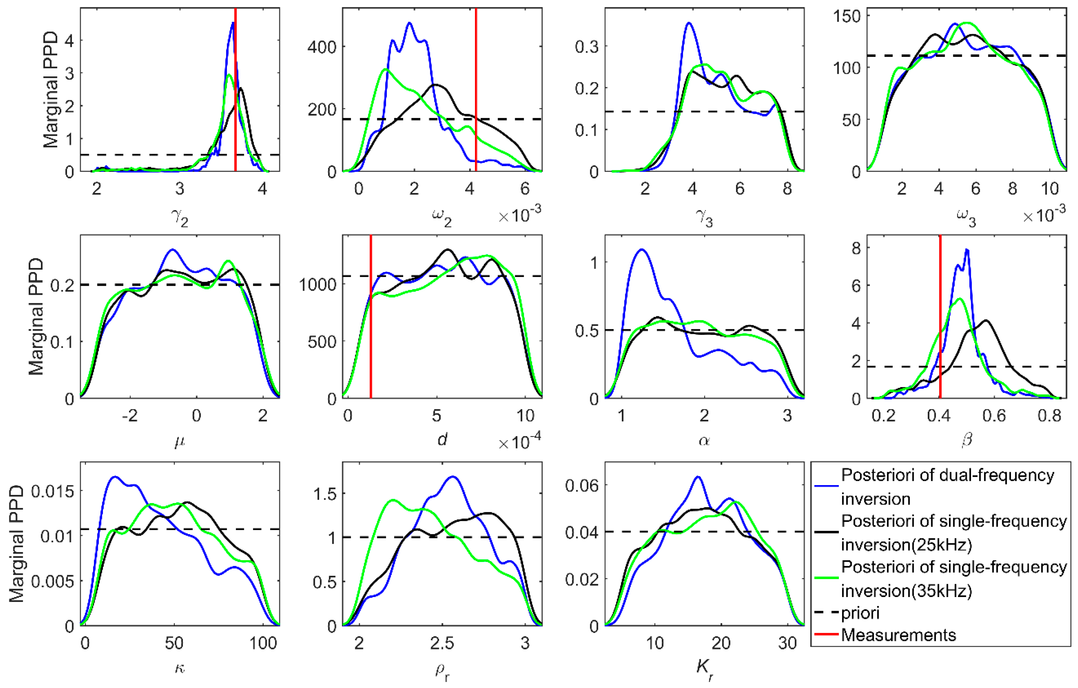
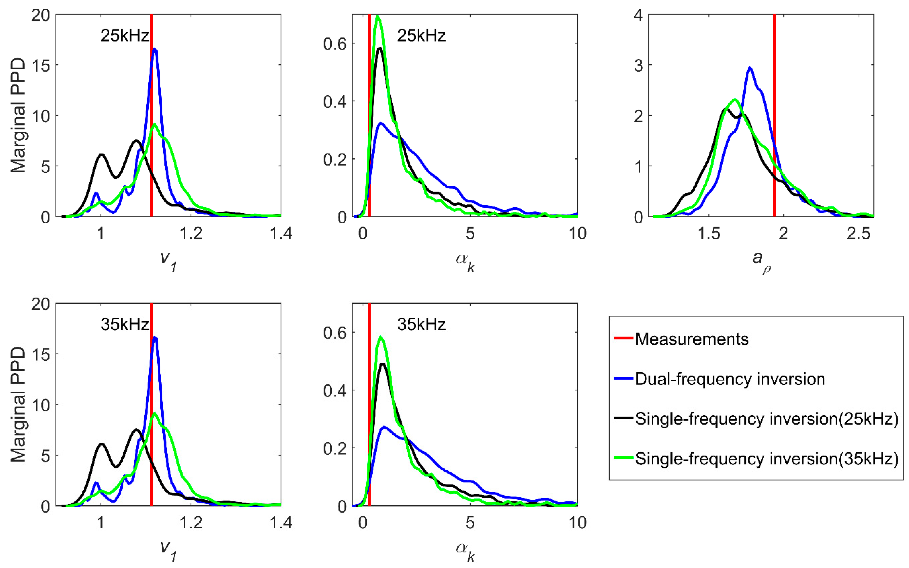
3.2.1. Parameter Uncertainty Analysis

Figure 3 displays the estimates of one-dimensional PPDs of model parameters for the three inversions. An inspection of the figure reveals that the roughness spectral exponent ${\gamma }_2$ and porosity $\beta$ were well resolved by the inversion, as their PPDs are much narrower than their respective priors. The roughness spectral strength ${\omega }_2$ and density fluctuation spectral exponent ${\gamma }_3$ were somewhat resolved by the inversion, as their PPDs changed appreciably from their respective priors. The PPDs of the remaining parameters only have a weak peak compared to their priors and provide an unreliable parameter inference. By comparing the three inversion results, it can be found that the PPDs of the dual-frequency inversion results are more concentrated than those of the single-frequency inversion results for the resolved parameters, and the reason is obvious, in that more data contains more information and can thus provide more accurate posterior estimates. The peak values of the PPDs of resolved parameters are different, and the reason for this is that each inversion is based on the best fitting with each set of backscattering strength data, which contains measurement error. The results of the dual-frequency inversion try to fit the measurements of the two frequencies and make a compromise. The comparison between the PPDs and the measured values show that ${\gamma }_2$ is the most accurate, ${\omega }_2$ and $\beta$ have appreciable deviations, and the parameter $d$ is unable to obtain a reliable estimate due to its insensitivity to backscattering strength.

The ratio of the sound velocity of sediment to water $v_1$, attenuation ${\mathsf{\alpha }}_k$ and the ratio of the mass density of sediment to water $a_{\rho }$ are indirectly inverted through uncertainty transfer, and the results are presented in Figure 4. The method substitutes all samples into the model to calculate these three quantities to form their respective sample sets which can be used for PPD estimation. There is no doubt that the sound velocity and attenuation of sound are frequency-dependent, which is not apparent in Figure 4 because of there being only two frequency points. The PPDs of the sound velocity ratio and density ratio for the three inversions in Figure 4 are similar to the results in Figure 3. The PPDs of the sound velocity ratio and density ratio of dual-frequency inversion results are much narrower than those of the other two single-frequency inversions. The PPDs of attenuation differ from those of the two parameters, and this could be attributed to the insensitivity of attenuation and errors of the measured data. Compared with the measurements, it can be seen that the MAP of the sound velocity ratio is the closest to the measured value, and there are appreciable deviations in attenuation and density ratio.

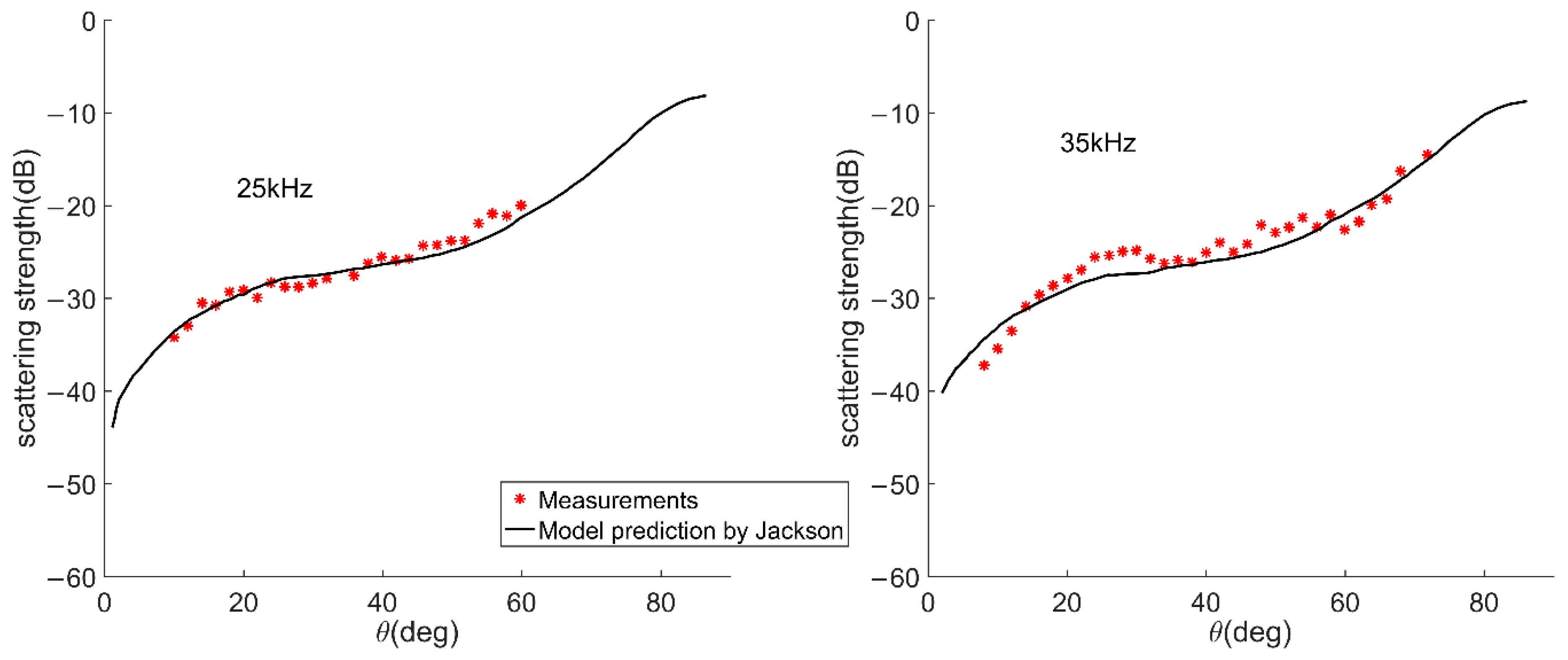
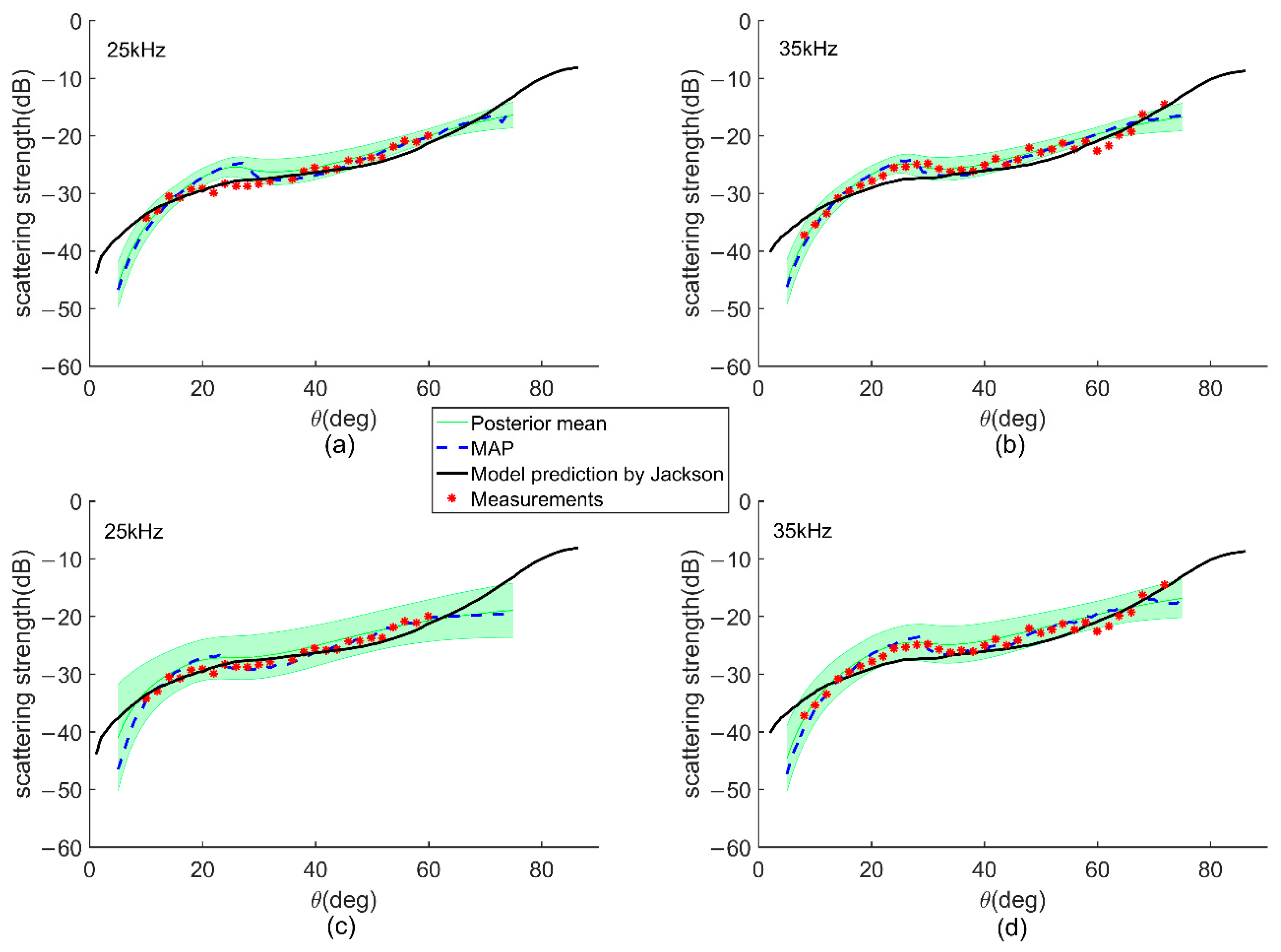
3.2.2. Model Prediction Uncertainty Analysis

Similarly, the samples obtained based on inversion can also be used to obtain the uncertainty of the predicted backscattering strength, which can be used for comparison with the measured values, and we can thus intuitively analyze the fitting performance of the inversion. The uncertainties of the predicted backscattering strength are represented by the colored part in Figure 5. The backscattering strength is calculated by the sample sets to obtain the backscattering strength sets of each angle at different frequencies (25 and 35 kHz), which were statistically transformed into a probability distribution and represented by a vertical color strip. All the vertical color strips for the angle range (5°–75°) were spliced together along the x-axis to form the subgraphs in Figure 5. On the whole, the uncertainty distributions of backscattering strength predicted by dual-frequency inversion are obviously narrower and more concentrated than those by single-frequency inversion. This is consistent with the PPDs of sensitive parameters in Figure 3. Nevertheless, the predicted values with maximum probabilities of single-frequency inversions are still well fitted to the corresponding measured values, although they have a wider uncertainty distribution, as shown in Figure 5c,d. In other words, dual-frequency inversion can reduce the uncertainty of partial model parameters and enhance the fitting performance between the predicted value and the measurements. Moreover, theoretically, we can also add more data at other frequencies to further reduce the uncertainties, but this is not necessarily worthwhile because reliable parameter estimation results have already been obtained and additional data require a higher measurement cost.

The backscattering strength predicted by dual-frequency inversion captures the characteristic drop near the critical angle, leading to a better-fitting performance at 35 kHz in Figure 5b than at 25 kHz in Figure 5a. The predicted value of 25 kHz in Figure 5a shows a characteristic drop which is not found in the measurements. This result is exactly the opposite of the fitting performance between Jackson’s prediction and the measurements, as described in Section 3.1. This is indeed the result of different errors in the backscattering strength measurements at the two frequencies and potential multiple optimal values of the inverse problem. Actually, Jackson’s prediction at 25 kHz obtained well-fitting performance with measurements, which led him to believe that volume scattering and roughness scattering were comparable, while the predicted scattering strength in this paper captured the unique drop characteristics of sandy sediment near the critical angle at 35 kHz, which means that roughness scattering is dominant. In the case of sandy sediment, it is more likely for us to accept the results with distinct drop characteristics, which has been confirmed by many field measurements. Nevertheless, both results are indeed reasonable when no volume scattering parameters are measured.

In order to compare the fitting performance of predicted backscattering strength more intuitively and quantitatively, the MAP and posterior mean of the backscattering strength sets of each angle at different frequencies are presented in Figure 6, where the median and width of the green strip represent the posterior mean and standard deviation, respectively. The standard deviations of backscattering strength predicted by dual-frequency inversion are obviously less than those by single-frequency inversion, and this is consistent with the results in Figure 5. For all the results in Figure 6, it can be seen that the posterior mean and MAP basically have the same trend except in the middle of the angle range, where appreciable differences can be observed. This also indicates that the predicted backscattering strength has more complex posterior distributions and greater uncertainty in this angle range.

Compared with the measurements, it can be obviously seen that the fitting performance of backscattering strength’s MAPs predicted by the inversion results and Jackson’s prediction have appreciable differences, which corresponds to the differences of PPD estimates for the parameter in Figure 3 and Figure 4. The predicted value of backscattering strength by dual-frequency inversion in this paper seems to fit the measurements from a different perspective compared with Jackson’s prediction. As analyzed above, the predicted results of dual-frequency inversion at 35 kHz have a better-fitting performance than Jackson’s results near the critical angle. On the contrary, Jackson’s results fit with the measured values better than the predicted results in this paper at 25 kHz in the same angle range.

For further analysis, the root-mean-square error (RMSE) between the measured value and corresponding estimates are calculated as shown in

Table 3. Root mean square error (RMSE) between the measured backscattering strength and Jackson’s prediction, and corresponding estimates of the MAP and posterior mean.

Inversion Type	RMSE Type	25kHz	35kHz
Dual-frequency	MAP and measurements	1.6	1.2
	Posterior mean and measurements	1.6	1.1
Jackson’s model	prediction and measurements	1.0	1.6
Single-frequency	MAP and measurements	1.0	1.3
	Posterior mean and measurements	1.3	1.3

. The RMSE of the MAP, posterior mean and measured values are close or even the same for both single-frequency and dual-frequency inversion. The RMSE of the MAP and measurements for single-frequency inversion results are equal to or less than those for Jackson’s results. Dual-frequency inversion reduces the RMSE at 35 kHz at the expense of increasing RMSE at 25 kHz, which can be clearly observed by comparing the results in Figure 6a,c. In general, the RMSE of the MAP, posterior mean, and measurements for dual-frequency inversion is similar to that of Jackson’s prediction and measurements, and they differ only in their RMSE values at different frequencies. This also indicates that the inverse problem is likely to have multiple optimal solutions. Therefore, the form of posterior distribution is more reliable and acceptable when compared with the results given by point estimation. We can assume that Jackson simply inverted the volume scattering parameters and took other measured model input parameters as prior information. The comparison of different predictions exactly confirms that the amount of prior information will have a significant impact on the inversion results in an inverse problem. Although the inversion in this paper only uses the simplest prior knowledge of uniform distribution and limited measured model outputs, we still achieve satisfactory inversion results where appreciable differences can be observed when compared with measured model inputs.

4. Conclusions

This study integrated the state-of-the-art MT-DREAM_(ZS) method to achieve an efficient and accurate solution of PPDs in model-based Bayesian geoacoustic inversion. The EDFM, which is a convenient approximation for the poroelastic model, and the published field measurements are adopted to implement the inversion. The PPDs of parameters indicate that the roughness spectral exponent ${\gamma }_2$, porosity $\beta$, roughness spectral strength ${\omega }_2$, and density fluctuation spectral exponent ${\gamma }_3$ can be resolved satisfactorily. By comparing the results of single-frequency and dual-frequency inversions, it can be seen that dual-frequency inversion results can provide more concentrated PPDs with fewer uncertainties. It can be considered that the inversion results given by the posterior probabilities based on the measurements and models adopted are reliable, although there may be a gap between the MAP and the measurements of the parameters due to the existence of measurement error. Meanwhile, the differences between the parameter MAP and the measured value are also reflected in the predicted outputs of the model. When comparing with Jackson’s prediction, the dual-frequency inversion has completed the matching with the measured backscattering strength from a different perspective, and they both have a similar fitting error level.

In fact, there is a marked difference between the predicted backscattering strength based on the dual-frequency inversion and Jackson’s prediction. The results in this paper match well with the measured backscattering strength at 35 kHz, while Jackson’s prediction matches well with the measurements at 25 kHz. This difference is essentially the difference in the estimation of the contribution between volume scattering and rough scattering to total scattering strength. By using volume scattering as a fitting parameter without measuring it, Jackson argues that the contributions of the two types of scattering to the total scattering at the Quinault site are comparable. By contrast, the Bayesian inversion results based on EDFM and MT-DREAM_(ZS) are well matched with the unique drop characteristics of the sandy sediment near the critical angle at 35 kHz, which means that rough scattering is considered to be dominant. The source of this difference is the measurement error of backscattering strength, and it can be considered that both results are reasonable in the absence of measured volume scattering parameters. Therefore, for an inverse problem, the solution given by Bayesian inversion is the most reasonable one due to the existence of multiple optimalities and measurement errors, and the way to make the solution more accurate is to provide more measured model outputs and prior information of model input based on limited measurement costs.

References

1. Anderson, J.T.; Van Holliday, D.; Kloser, R.; Reid, D.G.; Simard, Y. Acoustic seabed classification: Current practice and future directions. ICES J. Mar. Sci. 2008, 65, 1004–1011. [Google Scholar] [CrossRef]
2. Zhou, T.; Li, H.S.; Zhu, J.J.; Wei, Y.K. A geoacoustic estimation scheme based on bottom backscatter signals from multiple angles. Acta Phys. Sin.-Chin. Ed. 2014, 63. [Google Scholar] [CrossRef]
3. Yang, K.D.; Ma, Y.L. A geoacoustic inversion method based on bottom reflection signals. Acta Phys. Sin.-Chin. Ed. 2009, 58, 1798–1805. [Google Scholar]
4. Siemes, K.; Snellen, M.; Amiri-Simkooei, A.R.; Simons, D.G.; Hermand, J.-P. Predicting Spatial Variability of Sediment Properties from Hydrographic Data for Geoacoustic Inversion. IEEE J. Ocean. Eng. 2010, 35, 766–778. [Google Scholar] [CrossRef]
5. Haris, K.; Chakraborty, B.; De, C.; Prabhudesai, R.G.; Fernandes, W. Model-based seafloor characterization employing multi-beam angular backscatter data—A comparative study with dual-frequency single beam. J. Acoust. Soc. Am. 2011, 130, 3623–3632. [Google Scholar] [CrossRef] [PubMed]
6. Thorsos, E.I.; Jackson, D.R. Thirty Years of Progress in Theory and Modeling of Sea Surface and Seabed Scattering. Aip. Conf. Proc. 2012, 1495, 127–149. [Google Scholar]
7. Williams, K.L.; Thorsos, E.I.; Jackson, D.R.; Hefner, B.T. Thirty years of sand acoustics: A perspective on experiments, models and data/model comparisons. Aip. Conf. Proc. 2012, 1495, 166–192. [Google Scholar]
8. Jackson, D.R.; Briggs, K.B. High-frequency bottom backscattering: Roughness versus sediment volume scattering. J. Acoust. Soc. Am. 1992, 92, 962–977. [Google Scholar] [CrossRef]
9. Jackson, D.R.; Briggs, K.B.; Williams, K.L.; Richardson, M.D. Tests of models for high-frequency seafloor backscatter. IEEE J. Ocean. Eng. 1996, 21, 458–470. [Google Scholar] [CrossRef]
10. Williams, K.L.; Jackson, D.R. Bistatic bottom scattering: Model, experiments, and model/data comparison. J. Acoust. Soc. Am. 1998, 103, 169–181. [Google Scholar] [CrossRef]
11. Stoll, R.D. Sediment Acoustics. Lecture Notes in Earth Sciences; Springer: Berlin, Germany, 1989; pp. 1–101. [Google Scholar]
12. Williams, K.L.; Grochocinski, J.M.; Jackson, D.R. Interface scattering by poroelastic seafloors: First-order theory. J. Acoust. Soc. Am. 2001, 110, 2956–2963. [Google Scholar] [CrossRef]
13. Williams, K.L.; Jackson, D.R.; Thorsos, E.I.; Tang, D.J.; Briggs, K.B. Acoustic backscattering experiments in a well characterized sand sediment: Data/model comparisons using sediment fluid and Biot models. IEEE J. Ocean. Eng. 2002, 27, 376–387. [Google Scholar] [CrossRef]
14. Chotiros, N.P. Acoustics of the Seabed as a Poroelastic Medium; Springer International Publishing: Cham, Switzerland, 2017. [Google Scholar]
15. Williams, K.L. An effective density fluid model for acoustic propagation in sediments derived from Biot theory. J. Acoust. Soc. Am. 2001, 110, 2276–2281. [Google Scholar] [CrossRef] [PubMed]
16. Williams, K.L.; Jackson, D.R.; Thorsos, E.I.; Dajun, T.; Schock, S.G. Comparison of sound speed and attenuation measured in a sandy sediment to predictions based on the Biot theory of porous media. IEEE J. Ocean. Eng. 2002, 27, 413–428. [Google Scholar] [CrossRef]
17. Williams, K.L.; Jackson, D.R.; Dajun, T.; Briggs, K.B.; Thorsos, E.I. Acoustic Backscattering from a Sand and a Sand/Mud Environment: Experiments and Data/Model Comparisons. IEEE J. Ocean. Eng. 2009, 34, 388–398. [Google Scholar] [CrossRef]
18. Williams, K.L. Adding thermal and granularity effects to the effective density fluid model. J. Acoust. Soc. Am. 2013, 133, EL431–EL437. [Google Scholar] [CrossRef] [Green Version]
19. De, C.C.; Chakraborty, B. Model-Based Acoustic Remote Sensing of Seafloor Characteristics. IEEE Trans. Geosci. Remote 2011, 49, 3868–3877. [Google Scholar] [CrossRef]
20. Dosso, S.E.; Nielsen, P.L.; Harrison, C.H. Bayesian inversion of reverberation and propagation data for geoacoustic and scattering parameters. J. Acoust. Soc. Am. 2009, 125, 2867–2880. [Google Scholar] [CrossRef]
21. Dosso, S.E.; Dettmer, J. Bayesian matched-field geoacoustic inversion. Inverse Probl. 2011, 27, 55009. [Google Scholar] [CrossRef]
22. Chapman, N.R. Perspectives on Geoacoustic Inversion of Ocean Bottom Reflectivity Data. J. Mar. Sci. Eng. 2016, 4, 61. [Google Scholar] [CrossRef]
23. Yang, K.D.; Xiao, P.; Duan, R.; Ma, Y.L. Bayesian Inversion for Geoacoustic Parameters from Ocean Bottom Reflection Loss. J. Comput. Acoust. 2017, 25. [Google Scholar] [CrossRef]
24. Hastings, W.K. Monte Carlo Sampling Methods Using Markov Chains and Their Applications. Biometrika 1970, 57, 97. [Google Scholar] [CrossRef]
25. Haario, H.; Saksman, E.; Tamminen, J. Adaptive proposal distribution for random walk Metropolis algorithm. Comput. Stat. 1999, 14, 375–395. [Google Scholar] [CrossRef]
26. Haario, H.; Saksman, E.; Tamminen, J. An adaptive Metropolis algorithm. Bernoulli 2001, 7, 223–242. [Google Scholar] [CrossRef]
27. Haario, H.; Laine, M.; Mira, A.; Saksman, E. DRAM: Efficient adaptive MCMC. Stat. Comput. 2006, 16, 339–354. [Google Scholar] [CrossRef]
28. Metropolis, N.; Rosenbluth, A.W.; Rosenbluth, M.N.; Teller, A.H.; Teller, E. Equation of State Calculations by Fast Computing Machines. J. Chem. Phys. 1953, 21, 1087–1092. [Google Scholar] [CrossRef] [Green Version]
29. Vrugt, J.A.; Gupta, H.V.; Bouten, W.; Sorooshian, S. A Shuffled Complex Evolution Metropolis algorithm for optimization and uncertainty assessment of hydrologic model parameters. Water Resour. Res. 2003, 39, 113–117. [Google Scholar] [CrossRef]
30. Braak, C.J.F.T. A Markov Chain Monte Carlo version of the genetic algorithm Differential Evolution: Easy Bayesian computing for real parameter spaces. Stat. Comput. 2006, 16, 239–249. [Google Scholar] [CrossRef]
31. Vrugt, J.A.; Braak, C.J.F.T.; Diks, C.G.H.; Robinson, B.A.; Hyman, J.M.; Higdon, D. Accelerating Markov Chain Monte Carlo Simulation by Differential Evolution with Self-Adaptive Randomized Subspace Sampling. Int. J. Nonlinear Sci. Numer. Simul. 2009, 10, 273–290. [Google Scholar] [CrossRef]
32. Vrugt, J.A. Markov chain Monte Carlo simulation using the DREAM software package: Theory, concepts, and MATLAB implementation. Environ. Model. Softw. 2016, 75, 273–316. [Google Scholar] [CrossRef] [Green Version]
33. Laloy, E.; Vrugt, J.A. High-dimensional posterior exploration of hydrologic models using multiple-try DREAM((ZS)) and high-performance computing. Water Resour. Res. 2012, 48. [Google Scholar] [CrossRef]
34. Dosso, S.E. Quantifying uncertainty in geoacoustic inversion. I. A fast Gibbs sampler approach. J. Acoust. Soc. Am. 2002, 111, 129–142. [Google Scholar] [CrossRef] [PubMed]
35. Dosso, S.E.; Nielsen, P.L. Quantifying uncertainty in geoacoustic inversion. II. Application to broadband, shallow-water data. J. Acoust. Soc. Am. 2002, 111, 143–159. [Google Scholar] [CrossRef] [PubMed]
36. Bonomo, A.L.; Isakson, M.J. A comparison of three geoacoustic models using Bayesian inversion and selection techniques applied to wave speed and attenuation measurements. J. Acoust. Soc. Am. 2018, 143, 2501. [Google Scholar] [CrossRef]
37. Zou, B.; Zhai, J.; Xu, J.; Li, Z.; Gao, S. A Method for Estimating Dominant Acoustic Backscatter Mechanism of Water-Seabed Interface via Relative Entropy Estimation. Math. Probl. Eng. 2018, 2018, 10. [Google Scholar] [CrossRef]
38. Zou, B.; Zhai, J.; Qi, Z.; Li, Z. A Comparison of Three Sediment Acoustic Models Using Bayesian Inversion and Model Selection Techniques. Remote Sens. 2019, 11, 562. [Google Scholar] [CrossRef]
39. Jackson, D.R.; Richardson, M.D. High-Frequency Seafloor Acoustics; Springer: New York, NY, USA, 2007. [Google Scholar]
40. Mourad, P.D.; Jackson, D.R. In High Frequency Sonar Equation Models for Bottom Backscatter and Forward Loss. In Proceedings of the OCEANS, Seattle, WA, USA, 18–21 September 1989. [Google Scholar]
41. Pouliquen, E.; Lyons, A.P.; Pace, N.G. Penetration of acoustic waves into rippled sandy seafloors. J. Acoust. Soc. Am. 2000, 108 Pt 1, 2071–2081. [Google Scholar] [CrossRef]
42. Zou, D.P.; Williams, K.L.; Thorsos, E.I. Influence of Temperature on Acoustic Sound Speed and Attenuation of Seafloor Sand Sediment. IEEE J. Ocean. Eng. 2015, 40, 969–980. [Google Scholar]
43. Dettmer, J.; Dosso, S.E.; Holland, C.W. Model selection and Bayesian inference for high-resolution seabed reflection inversion. J. Acoust. Soc. Am. 2009, 125, 706–716. [Google Scholar] [CrossRef]
44. Dettmer, J.; Holland, C.W.; Dosso, S.E. Analyzing lateral seabed variability with Bayesian inference of seabed reflection data. J. Acoust. Soc. Am. 2009, 126, 56–69. [Google Scholar] [CrossRef]
45. Jiang, Y.M.; Chapman, N.R. The impact of ocean sound speed variability on the uncertainty of geoacoustic parameter estimates. J. Acoust. Soc. Am. 2009, 125, 2881–2895. [Google Scholar] [CrossRef] [PubMed]
46. Lucka, F. Fast Gibbs sampling for high-dimensional Bayesian inversion. Inverse Probl. 2016, 32, 115019. [Google Scholar] [CrossRef] [Green Version]
47. Guo, X.-L.; Yang, K.-D.; Ma, Y.-L. Geoacoustic Inversion for Bottom Parameters via Bayesian Theory in Deep Ocean. Chin. Phys. Lett. 2017, 34, 034301. [Google Scholar] [CrossRef]
48. Laloy, E.; Fasbender, D.; Bielders, C.L. Parameter optimization and uncertainty analysis for plot-scale continuous modeling of runoff using a formal Bayesian approach. J. Hydrol. 2010, 380, 82–93. [Google Scholar] [CrossRef]
49. Laloy, E.; Weynants, M.; Bielders, C.L.; Vanclooster, M.; Javaux, M. How efficient are one-dimensional models to reproduce the hydrodynamic behavior of structured soils subjected to multi-step outflow experiments? J. Hydrol. 2010, 393, 37–52. [Google Scholar] [CrossRef]
50. Scharnagl, B.; Vrugt, J.A.; Vereecken, H.; Herbst, M. Information content of incubation experiments for inverse estimation of pools in the Rothamsted carbon model: A Bayesian perspective. Biogeosciences 2010, 7, 763–776. [Google Scholar] [CrossRef]
51. Liu, J.S.; Liang, F.; Wong, W.H. The Multiple-Try Method and Local Optimization in Metropolis Sampling. J. Am. Stat. Assoc. 2000, 95, 121–134. [Google Scholar] [CrossRef]
52. Gelman, A.; Rubin, D.B. Inference from Iterative Simulation Using Multiple Sequences. Stat. Sci. 1992, 7, 457–472. [Google Scholar] [CrossRef]
53. Boehme, H.; Chotiros, N.P. Acoustic backscattering at low grazing angles from the ocean bottom. J. Acoust. Soc. Am. 1988, 84, 1018–1029. [Google Scholar] [CrossRef]
54. Hefner, B.T.; Williams, K.L. Sound speed and attenuation measurements in unconsolidated glass-bead sediments saturated with viscous pore fluids. J. Acoust. Soc. Am. 2006, 120, 2538–2549. [Google Scholar] [CrossRef] [Green Version]
55. Hamilton, E.L. Compressional-Wave Attenuation in Marine Sediments. Geophysics 1972, 37, 620–646. [Google Scholar] [CrossRef]
Figure 1. Sketch of the distributed implementation of multiple-try differential evolution adaptive Metropolis(ZS) (MT-DREAM(ZS)).
Jmse 07 00372 g001
Figure 2. Comparison of the predicted backscattering strength by Jackson and measured data for the Quinault site.
Jmse 07 00372 g002
Figure 3. Estimates of one-dimensional marginal posterior probability distributions (PPDs) of model parameters.
Jmse 07 00372 g003
Figure 4. Estimates of one-dimensional marginal posterior probability distributions (PPDs) of compressional sound velocity of sediment to water, corresponding attenuation, and the ratio of the mass density of sediment to water.
Jmse 07 00372 g004
Figure 5. Comparison of Jackson’s prediction, measured data and uncertainties of (a) a backscattering strength of 25 kHz predicted by dual-frequency inversion, (b) backscattering strength of 35 kHz predicted by dual-frequency inversion, (c) backscattering strength of 25 kHz predicted by single-frequency (25 kHz) inversion, (d) backscattering strength of 35 kHz predicted by single-frequency (35 kHz) inversion.
Jmse 07 00372 g005
Figure 6. Comparison of Jackson’s prediction, measured data and maximum a posteriori (MAP), posterior mean of (a) a backscattering strength of 25 kHz predicted by dual-frequency inversion, (b) backscattering strength of 35 kHz predicted by dual-frequency inversion, (c) backscattering strength of 25 kHz predicted by single-frequency (25 kHz) inversion, (d) backscattering strength of 35 kHz predicted by single-frequency (35 kHz) inversion.
Jmse 07 00372 g006