Acknowledgments
Pre-storm data was provided by Versar, Inc. We thank the Assateague Island National Seashore staff and project partners for their input, including Monique Lafrance-Bartley, Bill Hulslander, Charles Roman, Mark Finkbeiner, Sara Stevens and Robin Baranowski. Field and lab work was made possible by Captains Kevin Beam and Evan Falgowski, Ellie Rothermel, Hannah Rusch, Danielle Ferraro, Stephanie Dohner, Tim Pileguard, Trevor Metz, Anna Schutschkow, Annie Daw, Jason Button, Leah Morgan, Drew Friedrichs, Rachel Dalafave, Alec Halbruner, Meghan Owings, Rachel Oidtman, and Alex Itin. We thank the Environmental Protection Agency Region III’s Ocean and Dredge Disposal Program Team, especially Renee Searfoss and Sherilyn Morgan Lau, for the loan of a Young grab sampler, as well as the University of Delaware’s Chris Sommerfield and Adam Marsh for the loans of additional laboratory and field equipment.
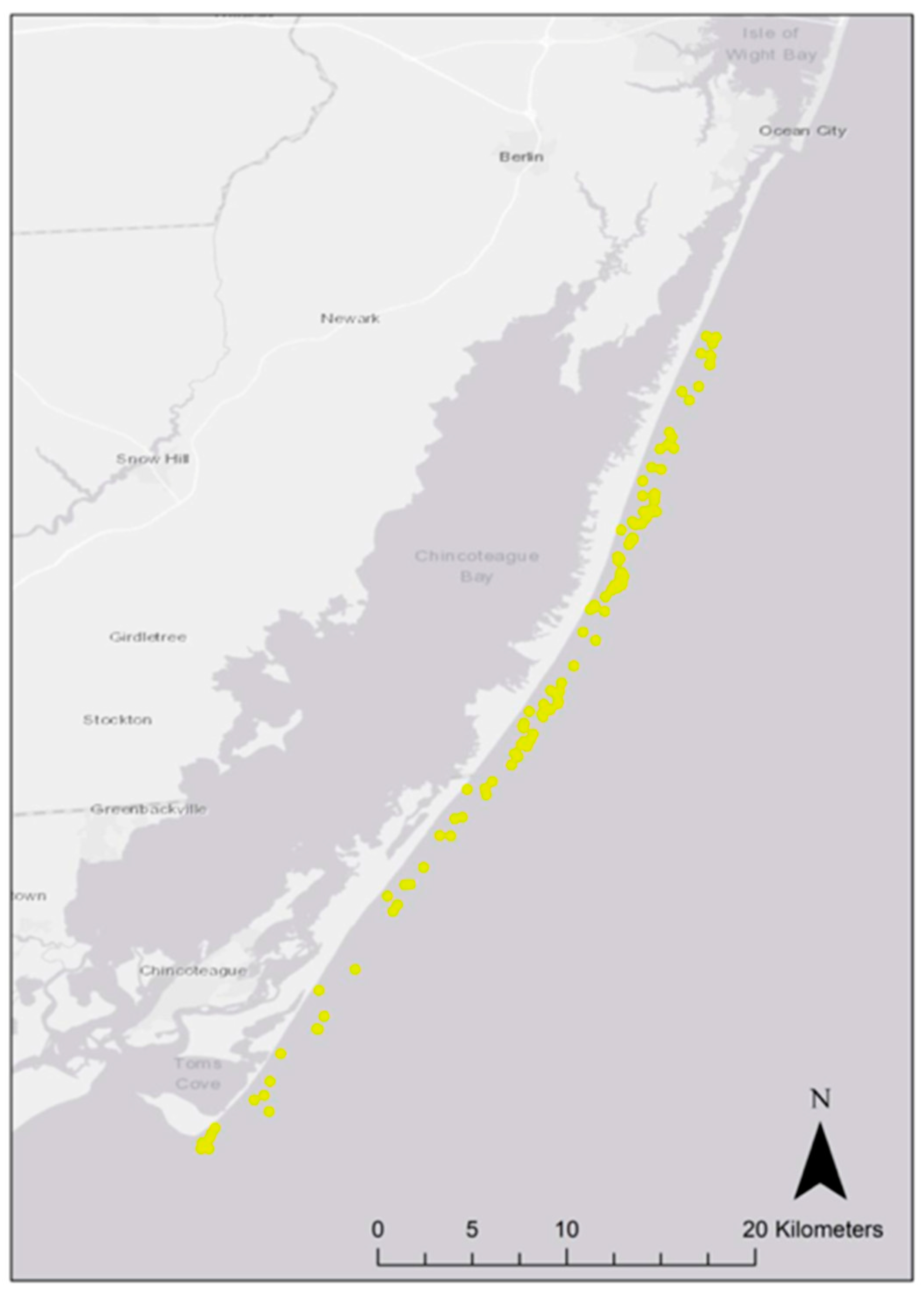
Figure 1.
Pre-Sandy (2011) survey sites (n = 125) sampled in October 2011 on the beach (n = 15) and subtidally up to 1 km offshore (n = 110) of Assateague Island National Seashore, Maryland.
Figure 1.
Pre-Sandy (2011) survey sites (n = 125) sampled in October 2011 on the beach (n = 15) and subtidally up to 1 km offshore (n = 110) of Assateague Island National Seashore, Maryland.
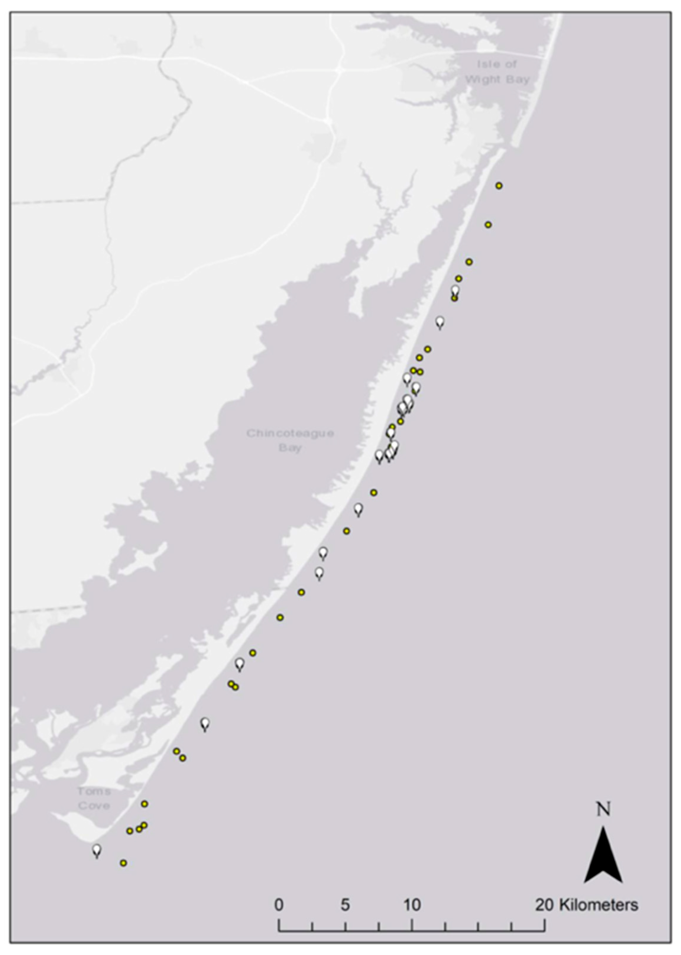
Figure 2.
Post-storm (n = 120 grabs) sampled in October 2014 (n = 60 grabs, white) and 2015 (n = 60 grabs, yellow), up to 1 km offshore of Assateague Island National Seashore survey sites, Maryland.
Figure 2.
Post-storm (n = 120 grabs) sampled in October 2014 (n = 60 grabs, white) and 2015 (n = 60 grabs, yellow), up to 1 km offshore of Assateague Island National Seashore survey sites, Maryland.
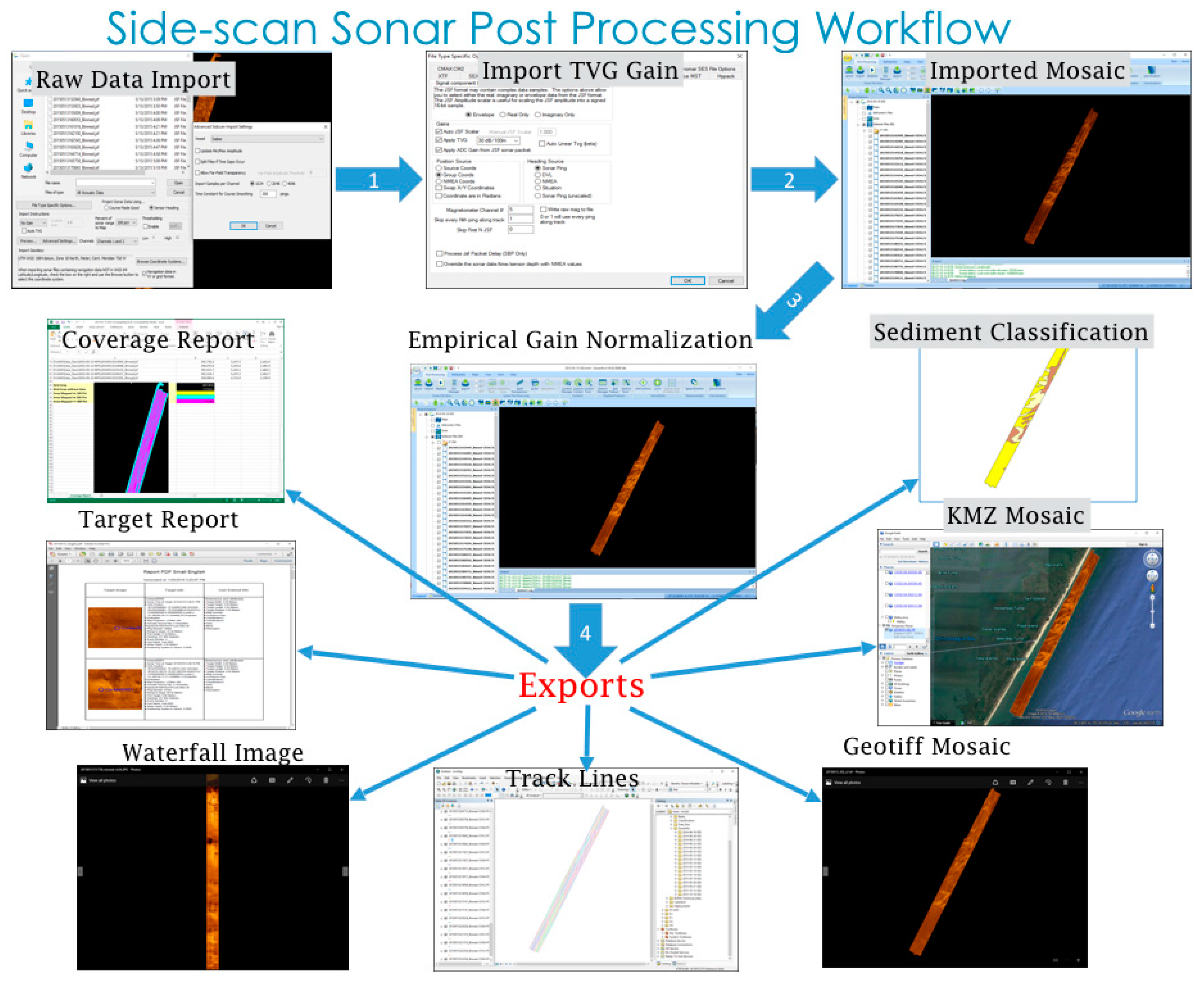
Figure 3.
Side-scan sonar post processing workflow used by the University of Delaware, Assateague Island National Seashore mapping project: From EdgeTech raw data to SonarWiz to shapefiles and Google Earth .kml data products.
Figure 3.
Side-scan sonar post processing workflow used by the University of Delaware, Assateague Island National Seashore mapping project: From EdgeTech raw data to SonarWiz to shapefiles and Google Earth .kml data products.
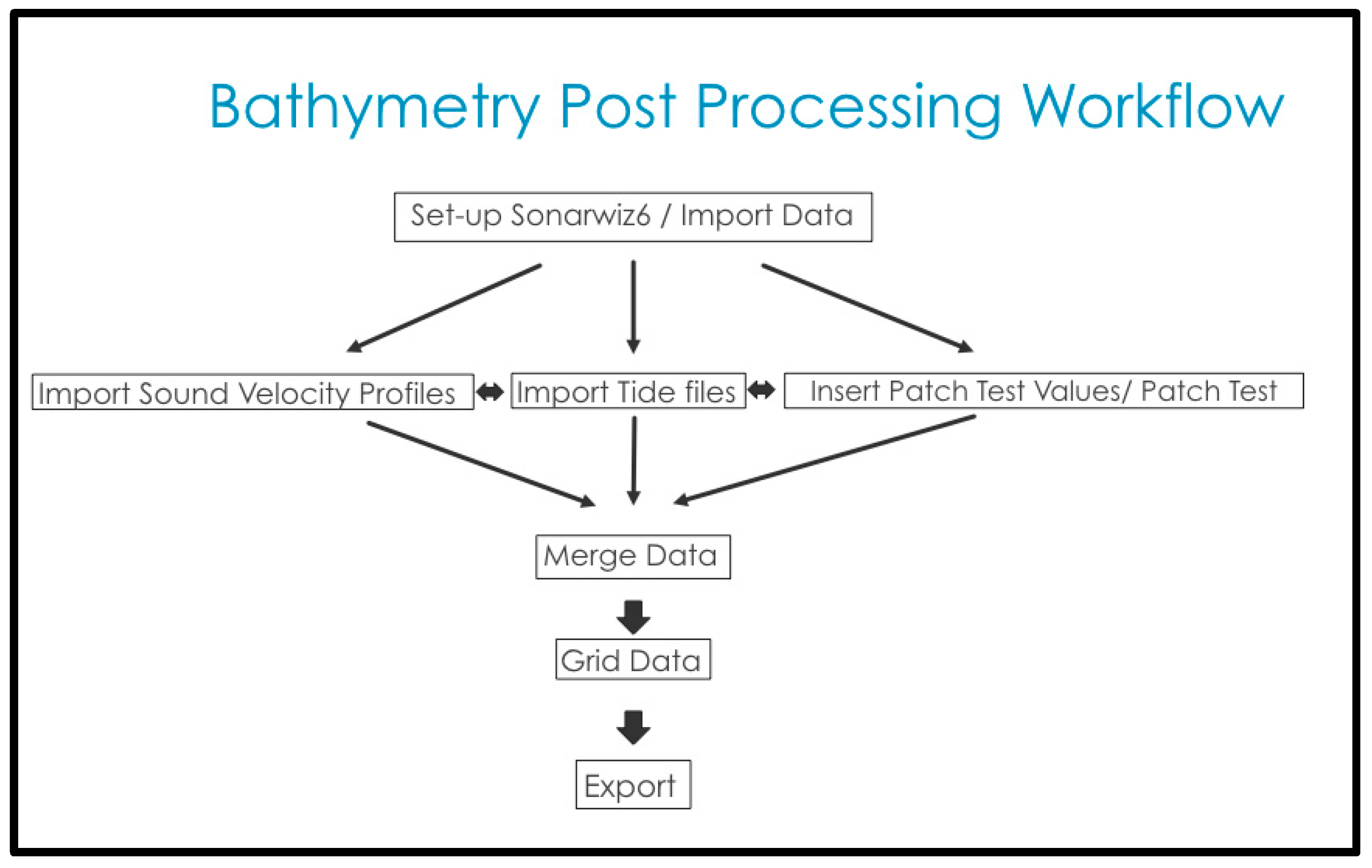
Figure 4.
Schematic of workflow used by the University of Delaware mapping team for multibeam bathymetry data from EdgeTech 6205 acquisition to gridded data products. Data collected as part of a submerged mapping study for Assateague Island National Seashore in 2014–2015.
Figure 4.
Schematic of workflow used by the University of Delaware mapping team for multibeam bathymetry data from EdgeTech 6205 acquisition to gridded data products. Data collected as part of a submerged mapping study for Assateague Island National Seashore in 2014–2015.
Figure 5.
Flow-chart of data processing steps for manually segmented side-scan sonar-sediment classification into a habitat map for Assateague Island National Seashore, developed by the University of Delaware 2014–2015.
Figure 5.
Flow-chart of data processing steps for manually segmented side-scan sonar-sediment classification into a habitat map for Assateague Island National Seashore, developed by the University of Delaware 2014–2015.
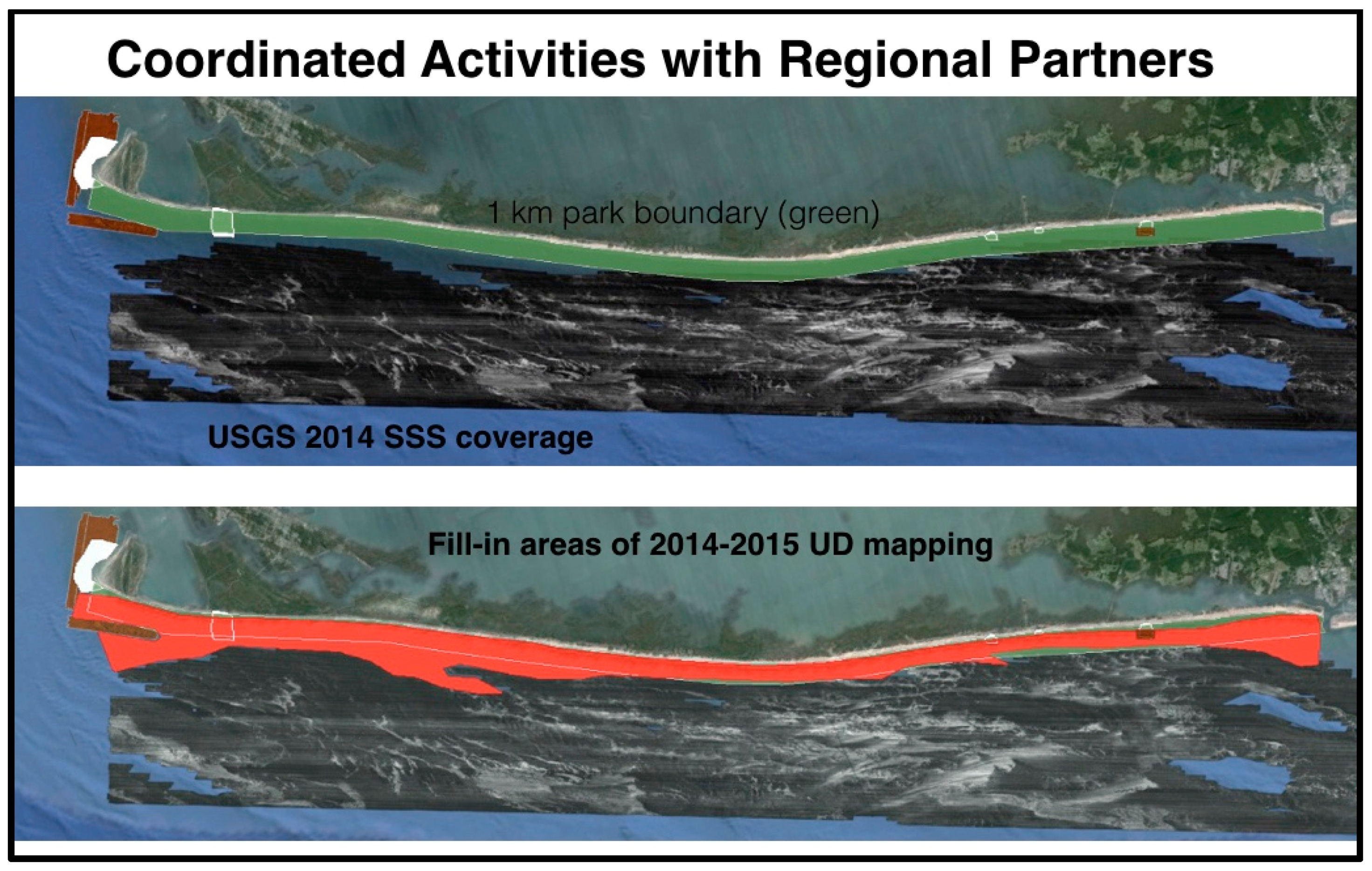
Figure 6.
Overview of study site area showing park boundary (green) and recent USGS coverage along with UD mapping team gap filling coverage (red).
Figure 6.
Overview of study site area showing park boundary (green) and recent USGS coverage along with UD mapping team gap filling coverage (red).
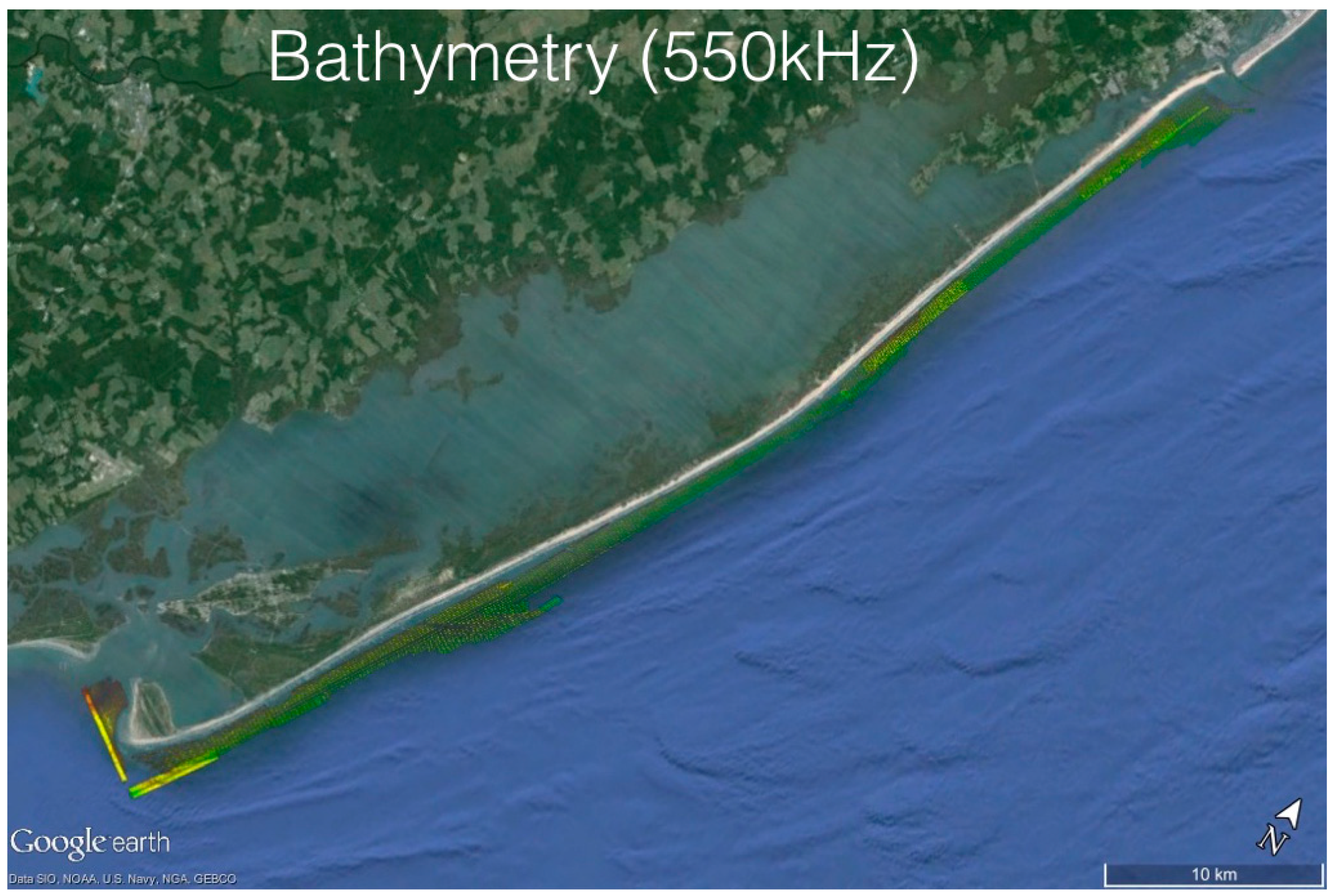
Figure 7.
Bathymetry mosaic (1m/pixel) from 2014–2015 acoustic surveys (550 kHz) for the entire study area. Notable features captured in the bathymetry included pronounced shore-attached oblique bars.
Figure 7.
Bathymetry mosaic (1m/pixel) from 2014–2015 acoustic surveys (550 kHz) for the entire study area. Notable features captured in the bathymetry included pronounced shore-attached oblique bars.
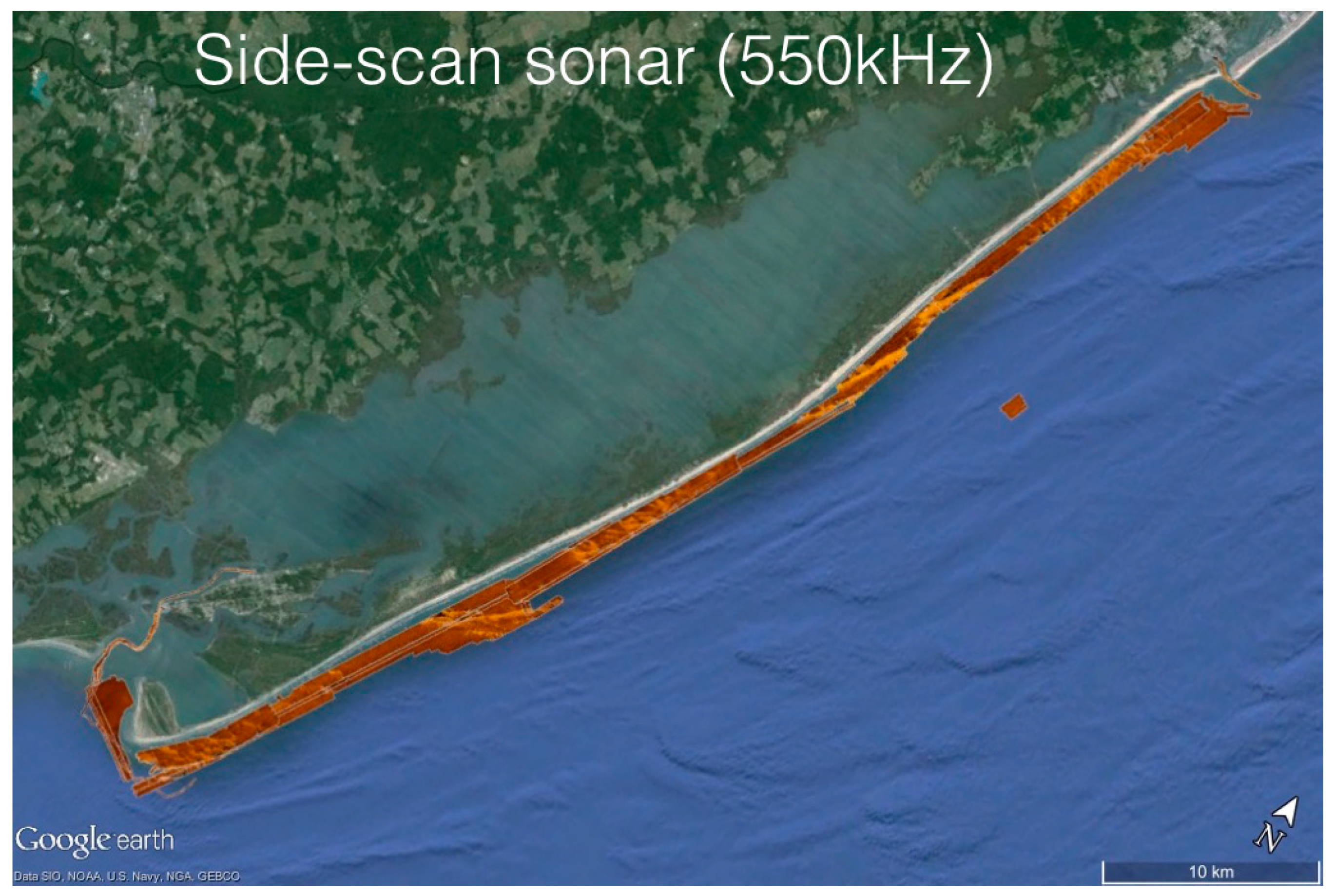
Figure 8.
Side-scan mosaic from 2014–2015 acoustic surveys for the entire study area.
Figure 8.
Side-scan mosaic from 2014–2015 acoustic surveys for the entire study area.
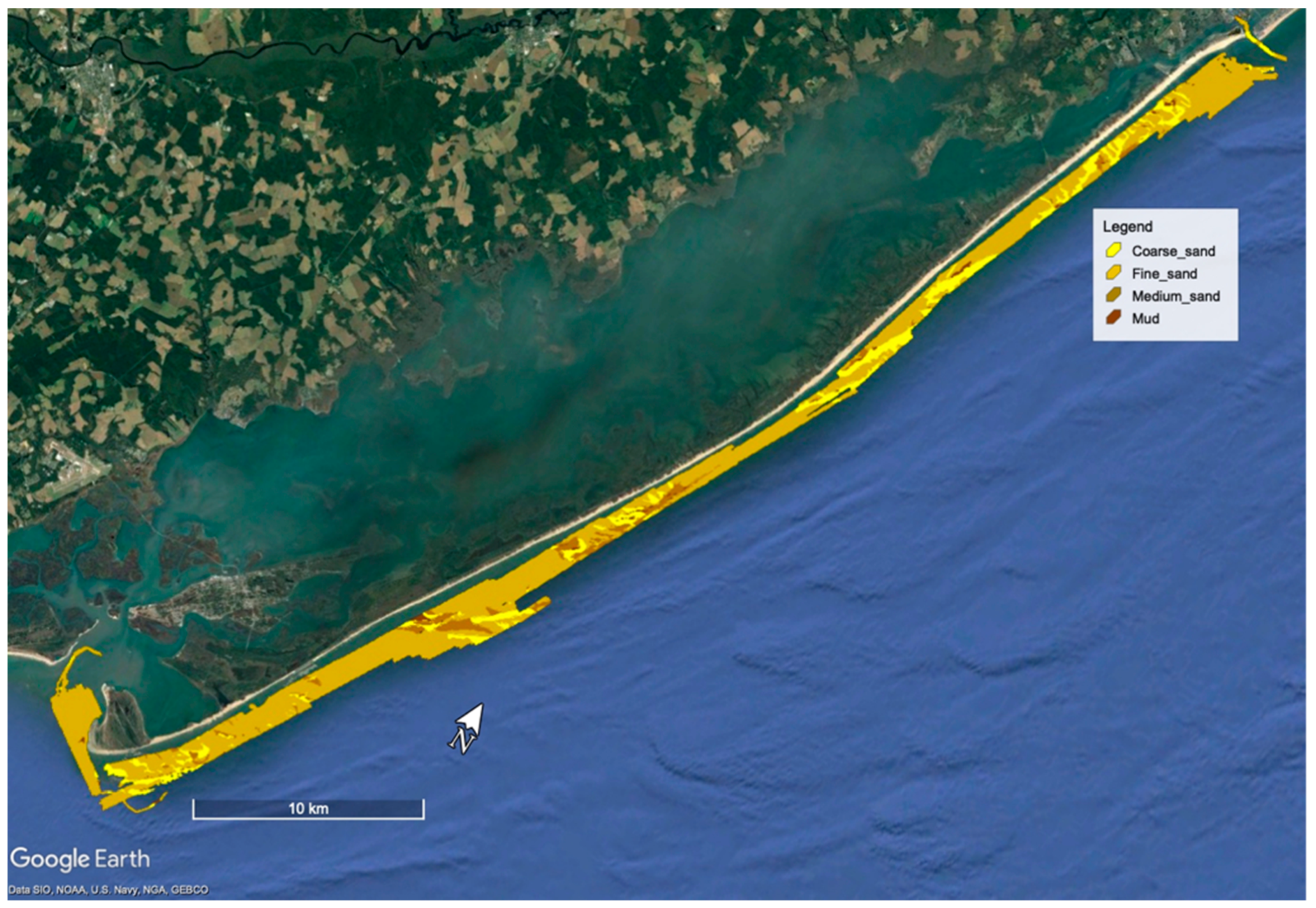
Figure 9.
Sediment classification from 2014–2015 for the entire study area. Four sediment classes (coarse and medium sand, mud, and fine sand) were recognized and shaded with different colors. Mapping survey conducted 2014–2015.
Figure 9.
Sediment classification from 2014–2015 for the entire study area. Four sediment classes (coarse and medium sand, mud, and fine sand) were recognized and shaded with different colors. Mapping survey conducted 2014–2015.
Figure 10.
Side-scan mosaic and classification shapefiles based on 2011 survey data.
Figure 10.
Side-scan mosaic and classification shapefiles based on 2011 survey data.
Figure 11.
May 2015 side-scan mosaic and sediment classification shapefile compared to 2011 from
Figure 9.
Figure 11.
May 2015 side-scan mosaic and sediment classification shapefile compared to 2011 from
Figure 9.
Figure 12.
October 2015 side-scan mosaic and sediment classification shapefile compared to May 2015 (
Figure 11) and 2011 (
Figure 10).
Figure 12.
October 2015 side-scan mosaic and sediment classification shapefile compared to May 2015 (
Figure 11) and 2011 (
Figure 10).
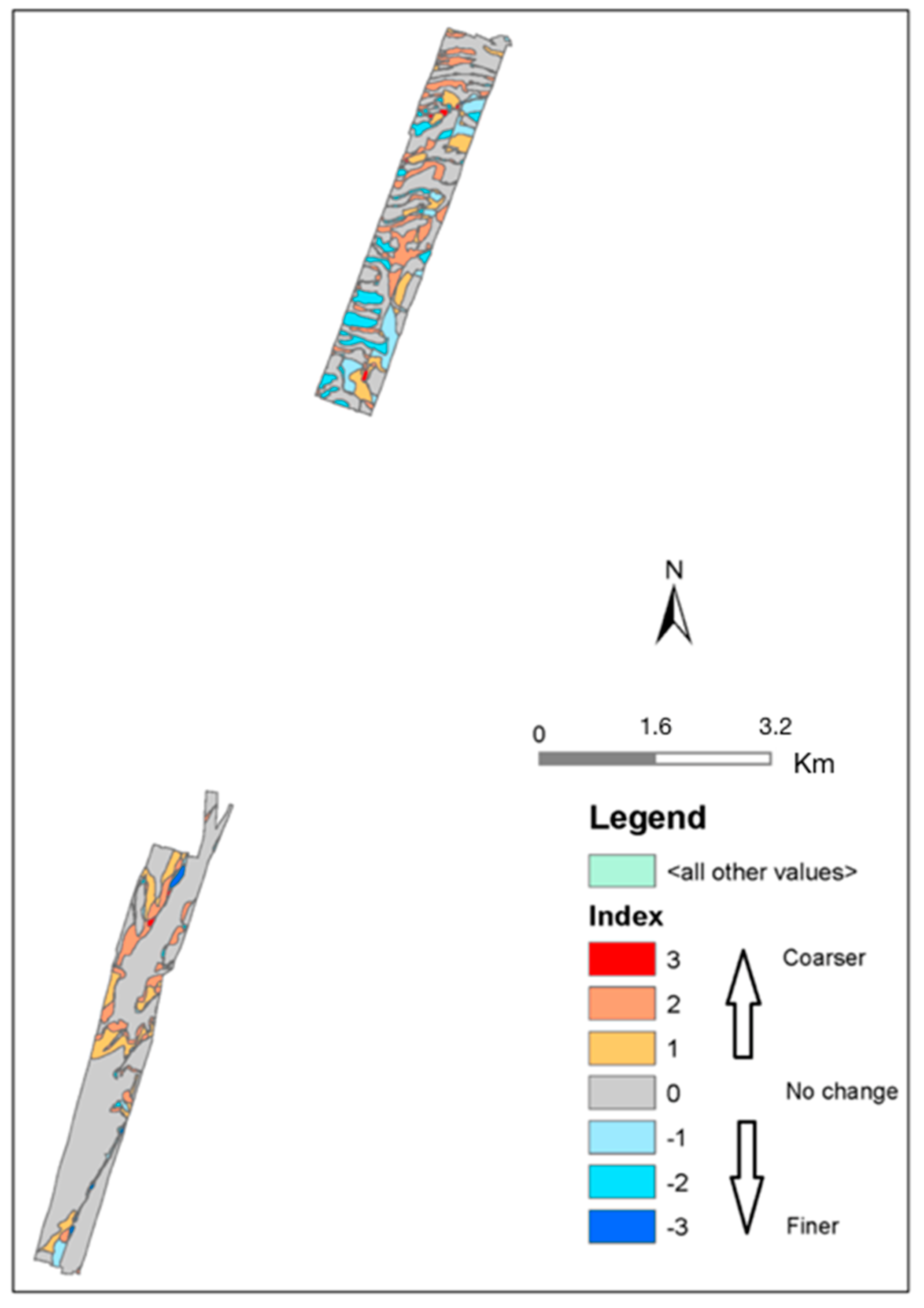
Figure 13.
Sediment property change map for submerged resources of Assateague Island National Seashore between May 2015 and October 2015. Positive sediment property change index means seafloor became coarser, negative sediment property change index means seafloor became finer and zero value means sediment texture did not change.
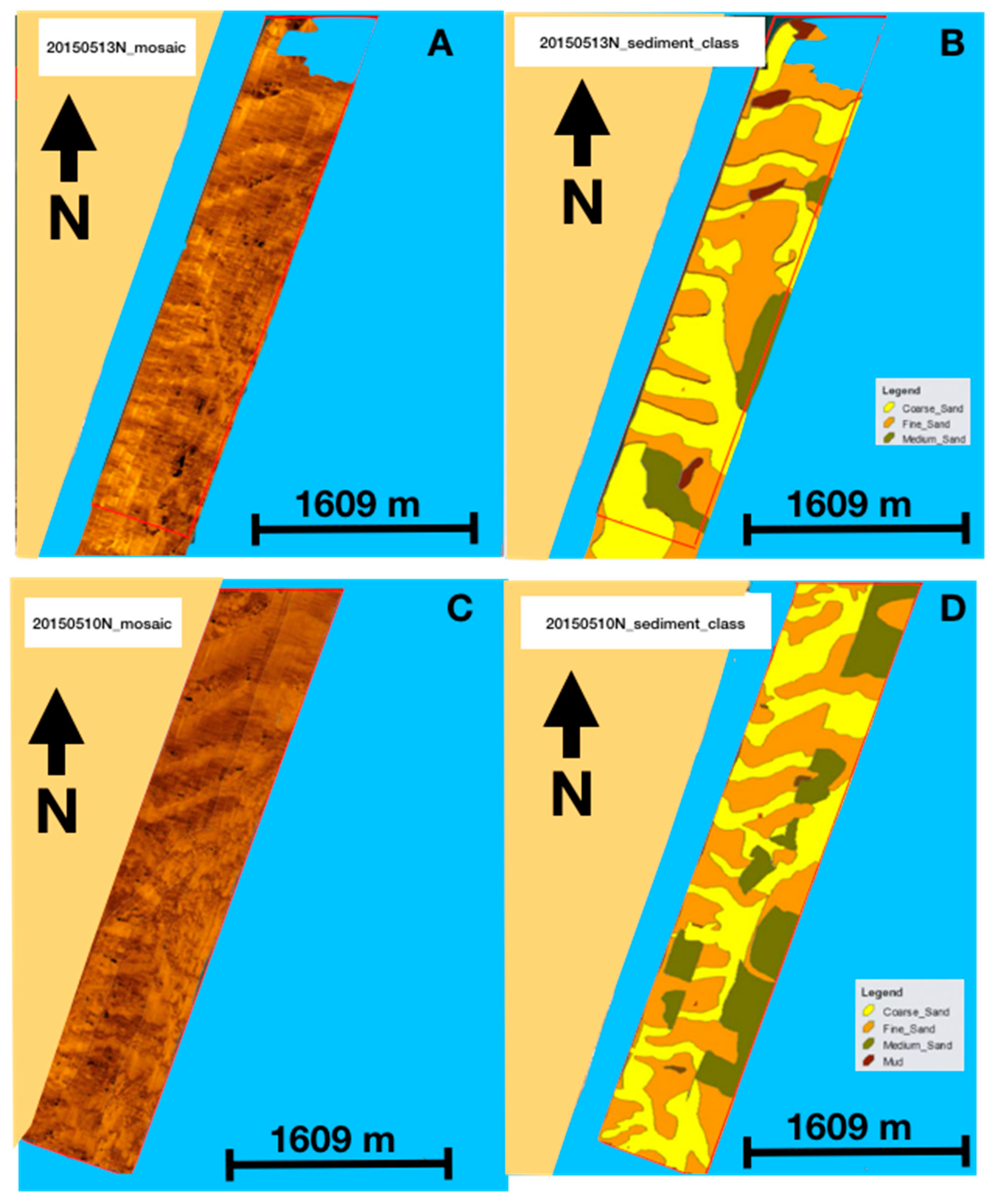
Figure 14.
Side-scan sonar mosaic interpretation, Assateague Island National Seashore, Maryland (A) side-scan sonar mosaics collected during 13 May 2015; (B) interpretation of side-scan sonar data collected in 13 May 2015; (C) side-scan sonar mosaics collected in October 2015; (D) interpretation of side-scan sonar mosaics collected in October 2015. Note that red polygons represent the same areas mapped during both 13 May 2015 and October 2015.
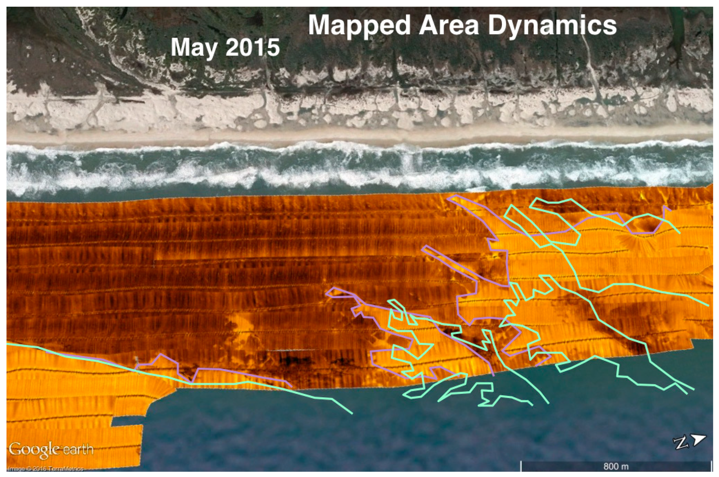
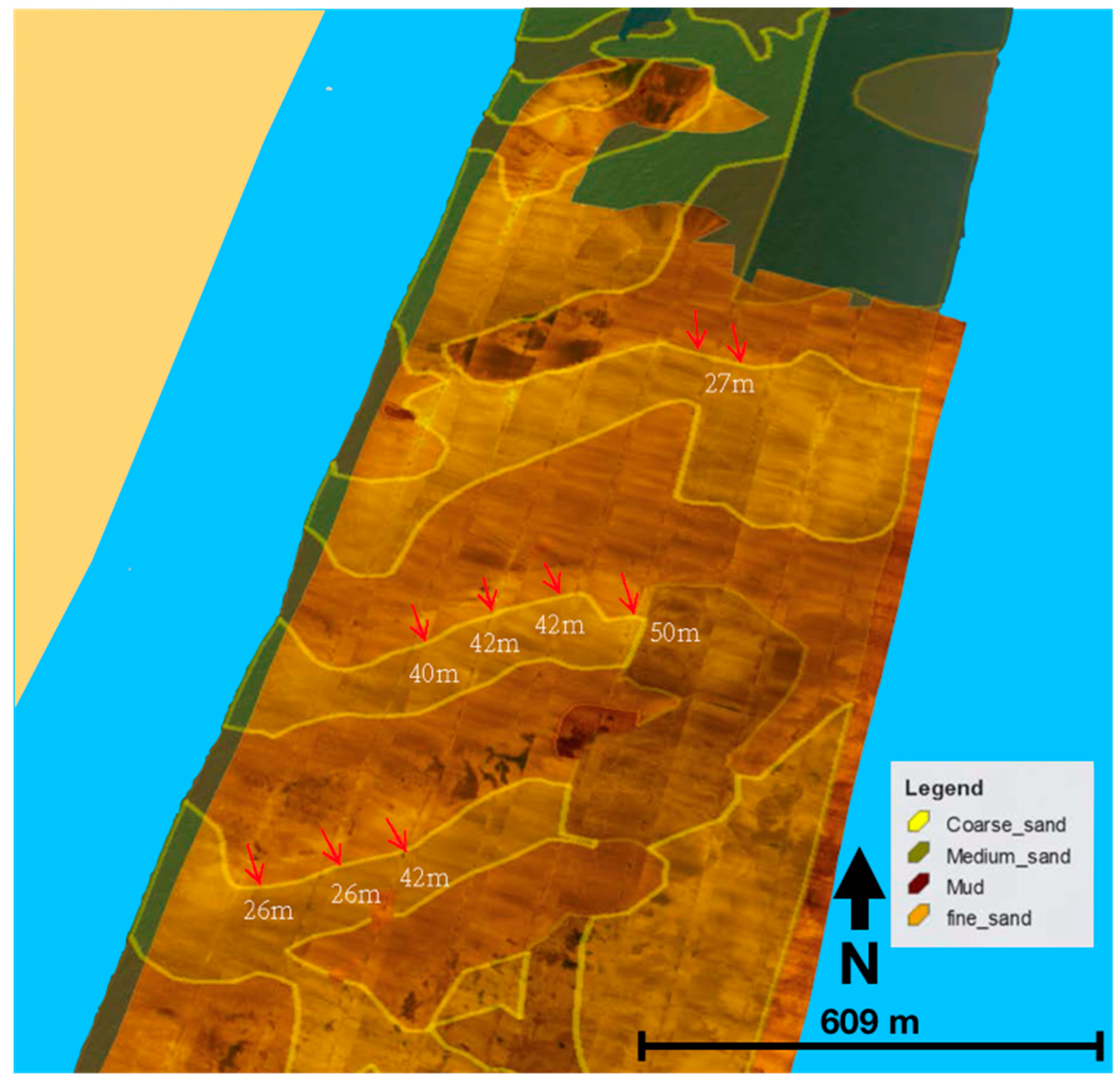
Figure 15.
Temporal changes in sediment class boundaries, Assateague Island National Seashore, Maryland. The underlying image on the bottom is the side-scan sonar mosaic collected during May 2015. Shaded polygons on the top represent sediment classes inferred from the side-scan sonar mosaics collected during October 2015. Note the southeastward shift (18–50 m) in the boundary of fine-coarse sand sediment classes.
Figure 16.
Side-scan sonar mosaic interpretation, Assateague Island National Seashore, Maryland. (A) Side-scan sonar mosaics collected during 13 May 2015; (B) Interpretation of side-scan sonar data collected in 13 May 2015; (C) side-scan sonar mosaics collected in October 2015; (D) Interpretation of side-scan sonar mosaics collected in October 2015. Note that red polygons represent the same areas mapped during both 13 May 2015 and October 2015.
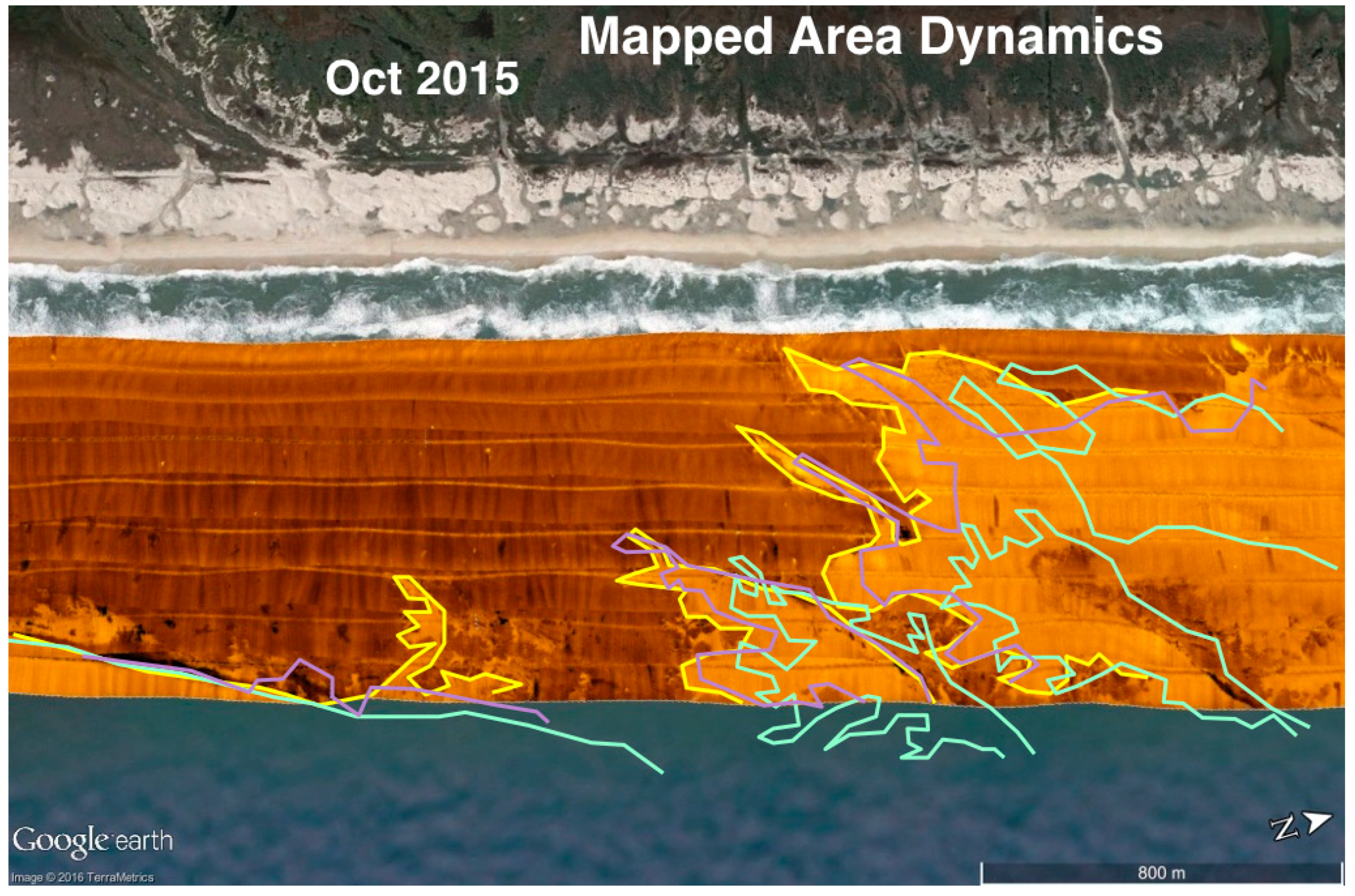
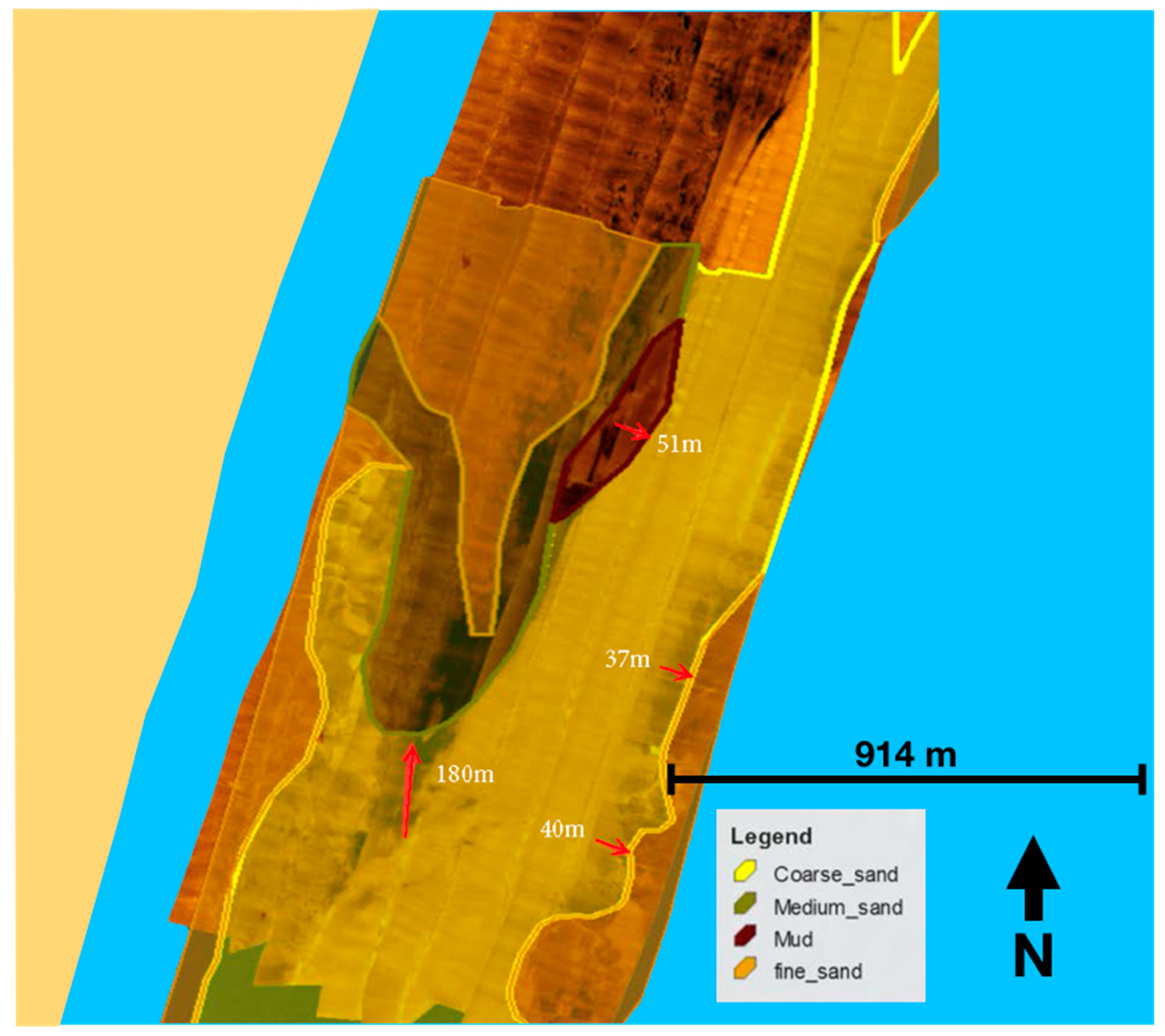
Figure 17.
Temporal changes in sediment class boundaries, Assateague Island National Seashore, Maryland. The profile in the bottom is the side-scan sonar mosaics collected during May 2015. Shaded polygons on the top represent sediment classes inferred from the side-scan sonar mosaics collected during October 2015. Please note the northward shift (180 m) in the boundary of mud-coarse sand sediment class and Southeastward shift (37–40m) in the boundary of fine–coarse sand sediment class.
Figure 18.
Side-scan sonar mosaic interpretation, Assateague Island National Seashore, Maryland. (A) Side-scan sonar mosaics collected during 14 May 2015; (B) interpretation of side-scan sonar data collected in 14 May 2015; (C) side-scan sonar mosaics collected in October 2015; (D) interpretation of side-scan sonar mosaics collected in October 2015. Note that red polygons represent the same areas mapped during both 14 May 2015 and October 2015.
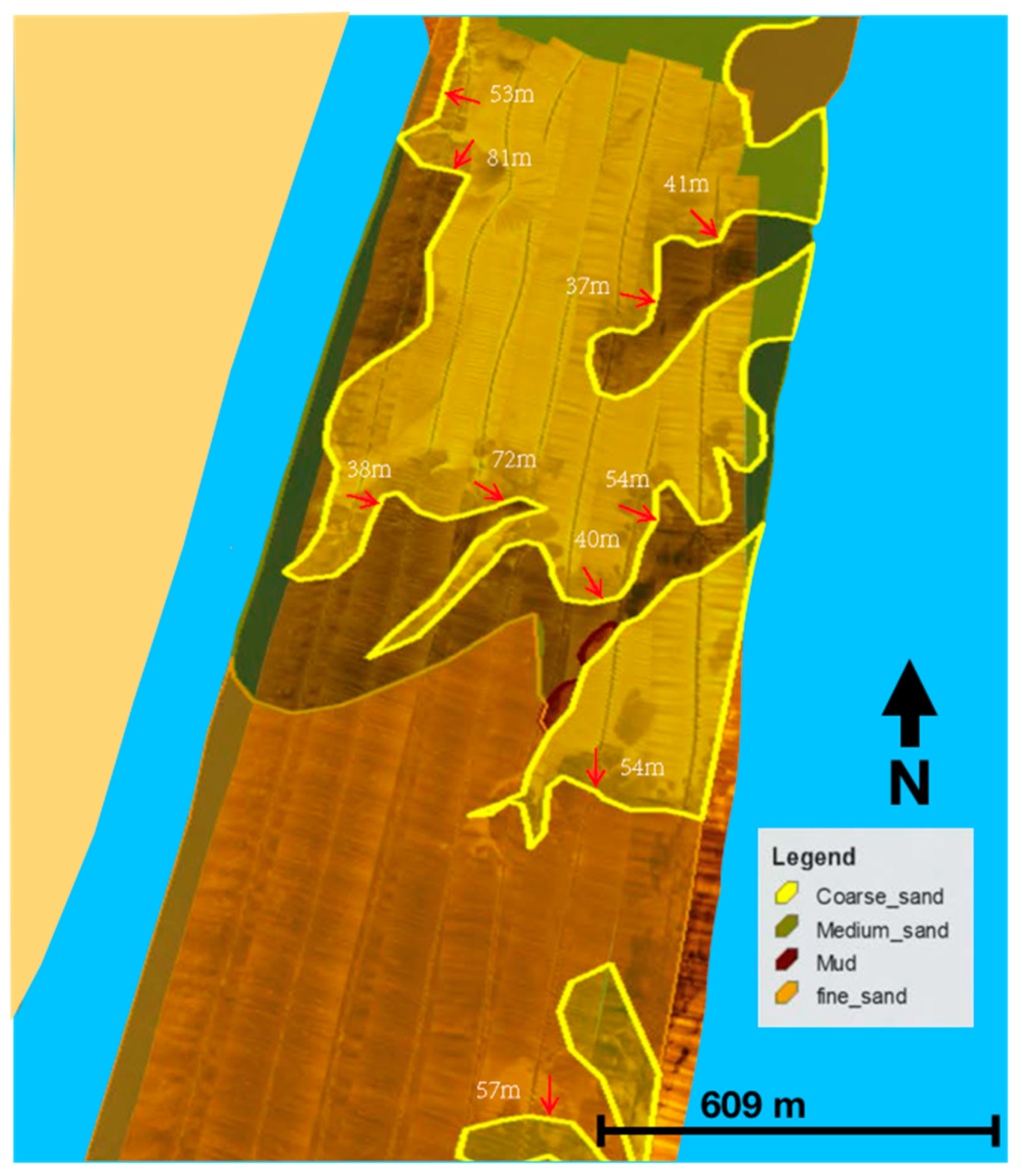
Figure 19.
Temporal changes in sediment class boundaries, Assateague Island National Seashore, Maryland. The profile in the bottom is the side-scan sonar mosaics collected during May 2015. Shaded polygons on the top represent sediment classes inferred from the side-scan sonar mosaics collected during October 2015. Please note the west-south-eastward shift (38–57 m) in the boundaries of fine–coarse sand sediment classes.
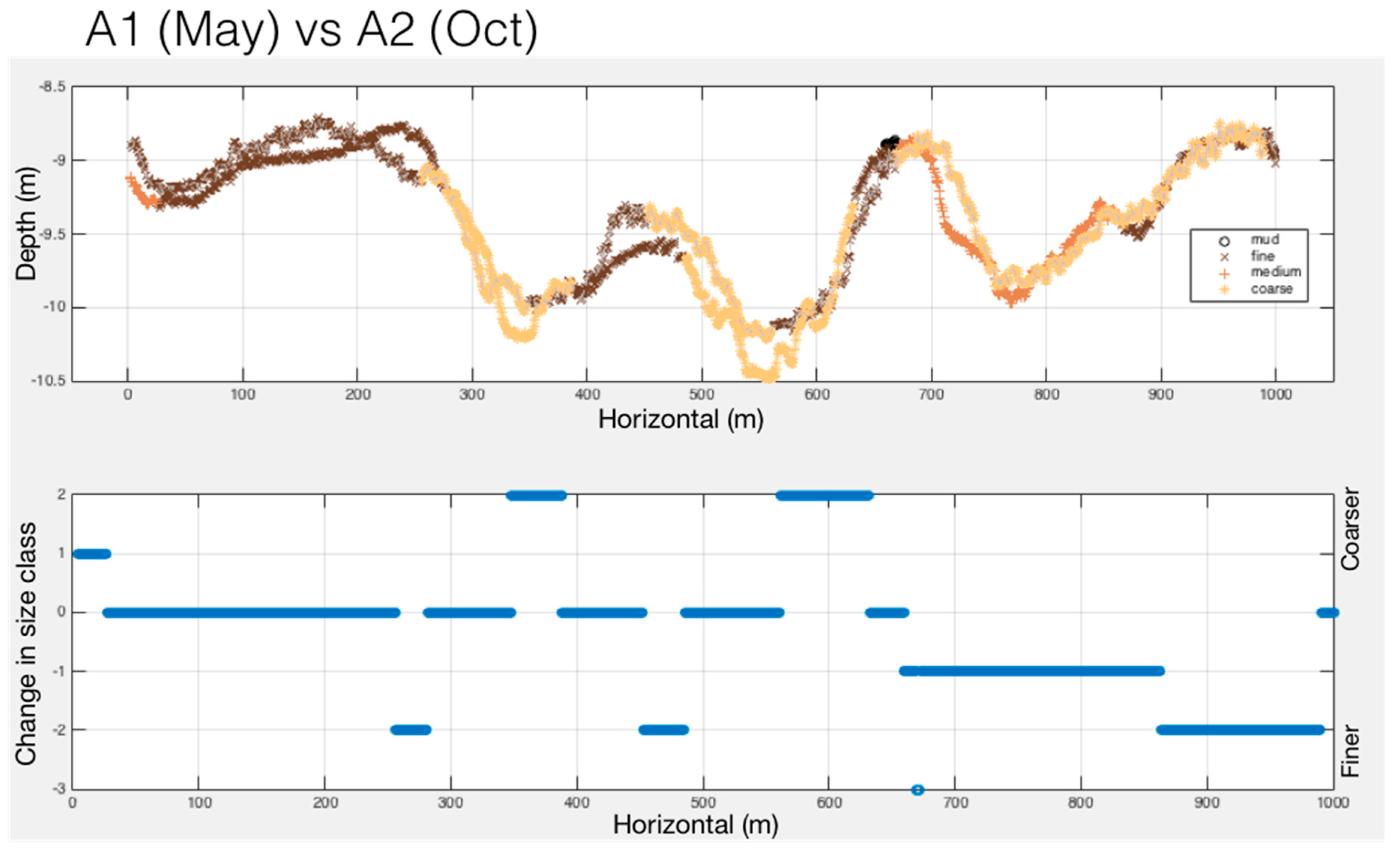
Figure 20.
Bathymetry profile change versus sediment class boundary shift after Hurricane Joaquin. Curved bathymetry profiles A1 (May 2015) and A2 (October 2015) are color coded according to the sediment types in the chart located in the top. Horizontal scale are meter in both panels, and vertical are meters in the top panel and size class index in the bottom panel. Sediment classes were indexed to 4, 1 representing the finest and 4 representing the coarsest. The chart in the bottom was generated by subtracting sediment type values of A1 (May 2015) from A2 (October 2015) to understand if the seafloor sediments are coarsening or fining with the lateral shift in bathymetry. Please note the coarsening of sediments in the top of the sand bars and fining of sediments in the trough. Inset scale is in meters on both axes.
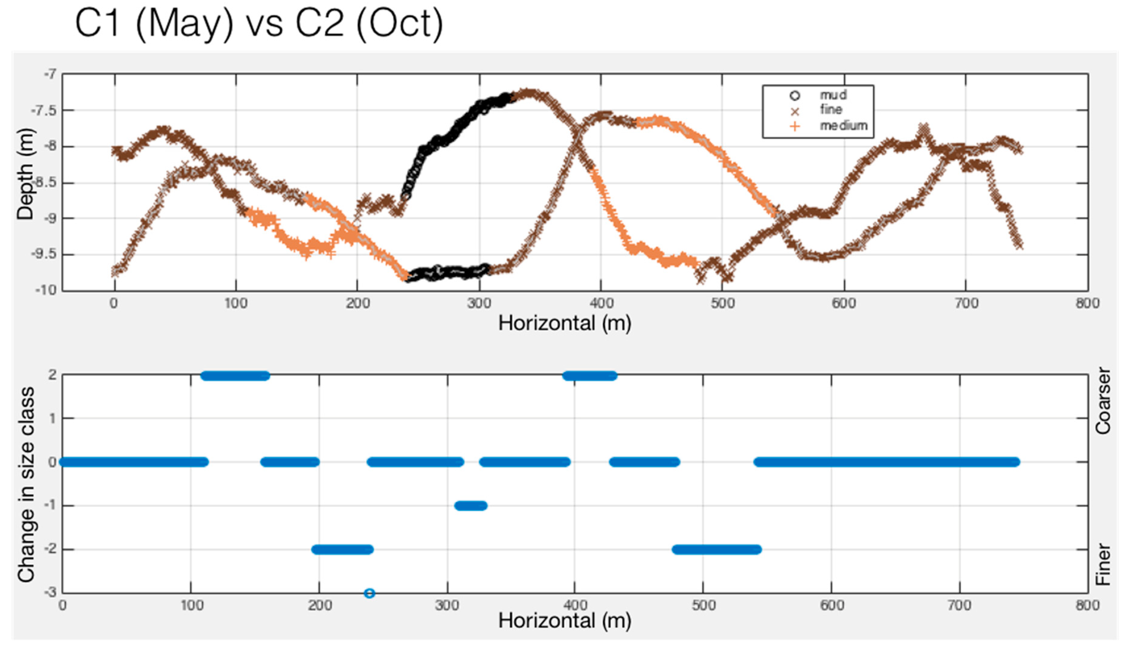
Figure 21.
Bathymetry profile change versus sediment class boundary shift after Hurricane Joaquin, Assateague Island National Seashore. Curved bathymetry profiles C1 (May 2015) and C2 (October 2015) in Figure 25 are color coded according to the sediment types in the chart located in the top. Horizontal scale are meters in both panels, and vertical are meters in the top panel and size class index in the bottom panel. Sediment classes were indexed from 1 to 4, 1 representing the finest and 4 representing the coarsest. The chart in the bottom was generated by subtracting sediment type values of C1 (May 2015) from C2 (October 2015) to understand if the seafloor sediments are coarsening or fining with the lateral shift in bathymetry. Please note the coarsening of sediments in the top of the sand bars and fining of sediments in the trough. Inset scale is in meters on both axes.
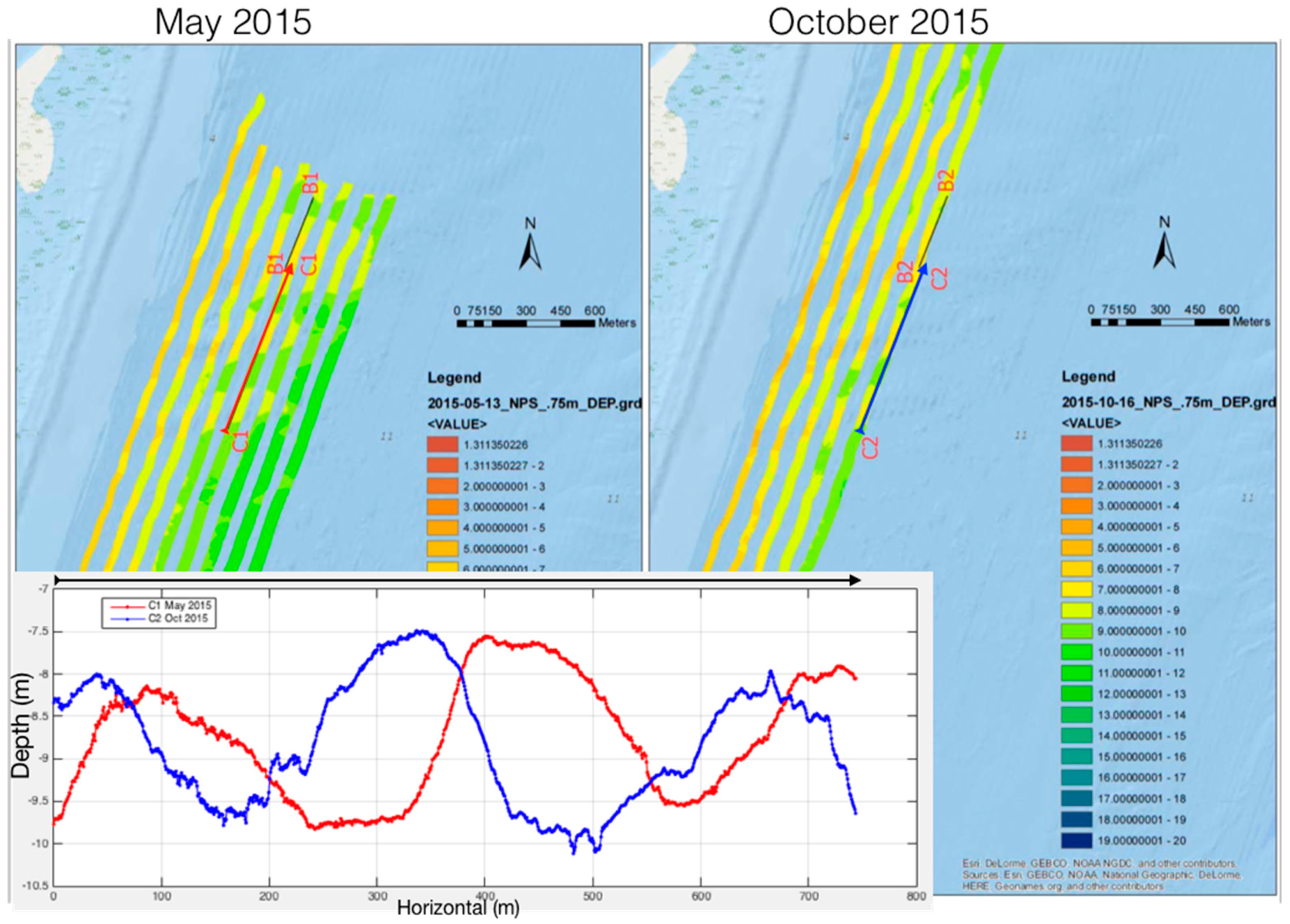
Figure 22.
Bathymetry profile change after Hurricane Joaquin, Assateague Island National Seashore, Maryland. Red curved line represents the bathymetry profile C1 in May 2015 and blue curved line represents the bathymetry profile C2 in October 2015. Please note the Southwestward lateral shift of sand bars in the bathymetry profile. Inset scale is in meters on both axes.
Figure 23.
Bathymetry profile change after Hurricane Joaquin. Red curved line represents the bathymetry profile G1 in May 2015 and blue curved line represents the bathymetry profile G2 in October 2015. Please note the change in surface roughness and the vertical offset in the bathymetry.
Figure 23.
Bathymetry profile change after Hurricane Joaquin. Red curved line represents the bathymetry profile G1 in May 2015 and blue curved line represents the bathymetry profile G2 in October 2015. Please note the change in surface roughness and the vertical offset in the bathymetry.
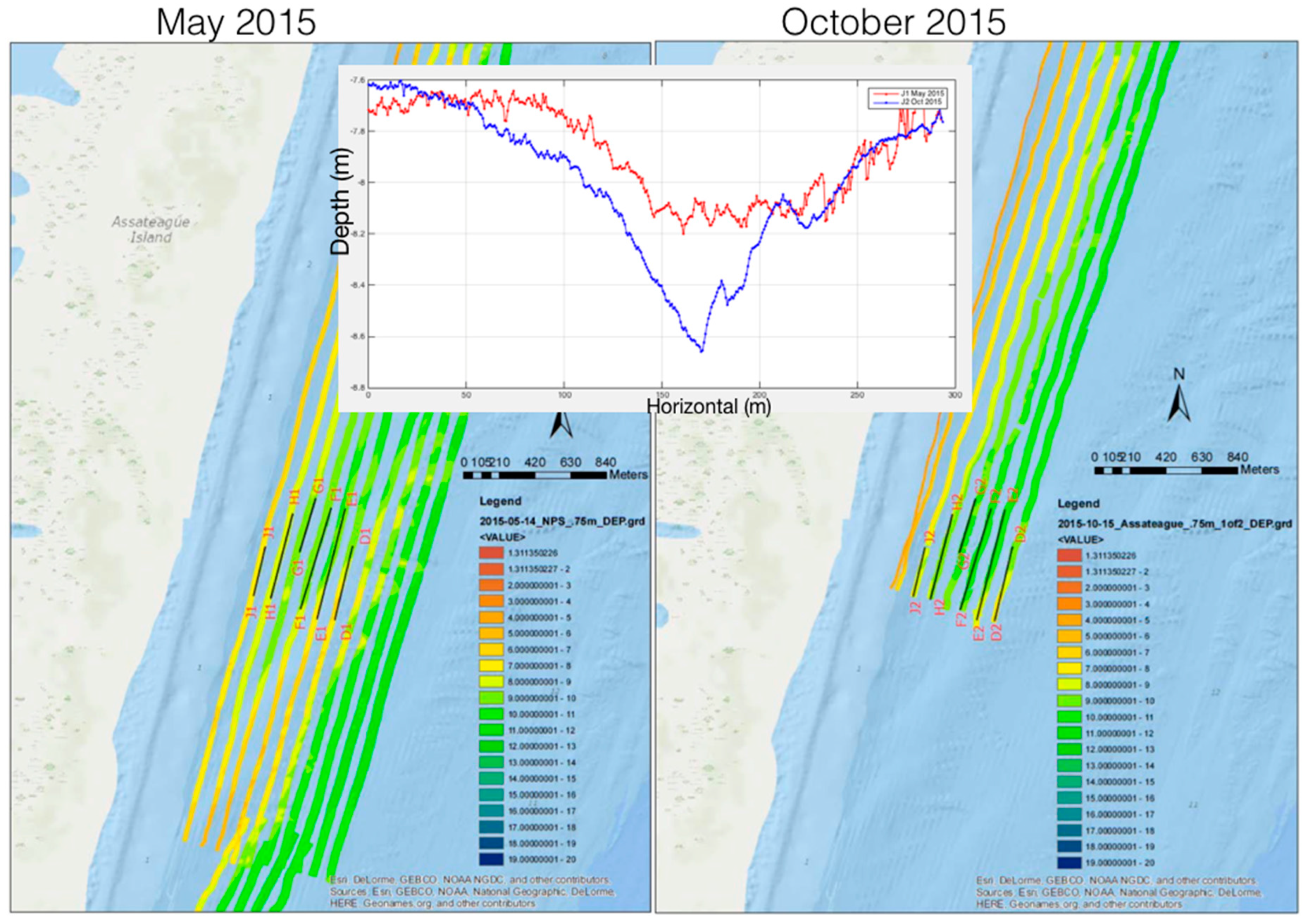
Figure 24.
Bathymetry profile change after Hurricane Joaquin. Red curved line represents the bathymetry profile J1 in May 2015 and blue curved line represents the bathymetry profile J2 in October 2015. Please note the axial incision in J2 profile.
Figure 24.
Bathymetry profile change after Hurricane Joaquin. Red curved line represents the bathymetry profile J1 in May 2015 and blue curved line represents the bathymetry profile J2 in October 2015. Please note the axial incision in J2 profile.
Figure 25.
Timeline of Storm events and seafloor mapping studies and resulting benthic habitat and morphology products.
Figure 25.
Timeline of Storm events and seafloor mapping studies and resulting benthic habitat and morphology products.
Figure 26.
Significant wave height (Hs) in meters (m) at offshore NDBC Buoy 44009 (38.461 N 74.703 W) between 2011–2016 including the passage of hurricanes Sandy and Joaquin near the study site.
Figure 26.
Significant wave height (Hs) in meters (m) at offshore NDBC Buoy 44009 (38.461 N 74.703 W) between 2011–2016 including the passage of hurricanes Sandy and Joaquin near the study site.
Table 1.
Surficial sediment distribution by class type based on the 2014–2015 habitat mapping expedition.
Table 1.
Surficial sediment distribution by class type based on the 2014–2015 habitat mapping expedition.
| Sediment Type | Classification Map Coverage % |
|---|
| Coarse Sand | 10% |
| Medium Sand | 1% |
| Fine Sand | 82% |
| Mud | 7% |


